SMaRT-OnlineWDN D5.6: Testing and optimisation of online simulation model for a miniaturised distribution network

(1)

HAL Id: hal-02601407

https://hal.inrae.fr/hal-02601407

Submitted on 16 May 2020

HAL is a multi-disciplinary open access archive for the deposit and dissemination of sci-entific research documents, whether they are pub-lished or not. The documents may come from teaching and research institutions in France or abroad, or from public or private research centers.

L’archive ouverte pluridisciplinaire HAL, est destinée au dépôt et à la diffusion de documents scientifiques de niveau recherche, publiés ou non, émanant des établissements d’enseignement et de recherche français ou étrangers, des laboratoires publics ou privés.

SMaRT-OnlineWDN D5.6: Testing and optimisation of

online simulation model for a miniaturised distribution

network

Jochen Deuerlein, Denis Gilbert, Nicolai Guth, Christian Kühnert, Lea Meyer

Harries, Idel Montalvo Arango, Reik Nitsche, Olivier Piller, Hervé Ung

To cite this version:

Jochen Deuerlein, Denis Gilbert, Nicolai Guth, Christian Kühnert, Lea Meyer Harries, et al.. SMaRT-OnlineWDN D5.6: Testing and optimisation of online simulation model for a miniaturised distribution network. [Research Report] irstea. 2015, pp.22. �hal-02601407�

(2)

Testing and optimisation of online simulation model for a miniaturised distribution network 31 March 2015

1

Deliverable 5.6

Testing and optimisation of online simulation

model for a miniaturised distribution network

Dissemination level: Public

WP 5

Online Simulation Model

30th April 2015

ANR reference project: ANR-11-SECU-006 BMBF reference project: 13N12180

Contact persons

Fereshte SEDEHIZADE [email protected]

(3)

Testing and optimisation of online simulation model for a miniaturised distribution

network 30 April 2015

2

WP 5 –

ONLINE-SIMULATION MODEL

D5.6 Testing and optimisation of online simulation model for a miniaturised

distribution network

List of Deliverable 5.6 contributors:

From 3S [WP5 leader]

Idel Montalvo ([email protected]) Jochen Deuerlein ([email protected]) Nicolai Guth ([email protected])

Lea Meyer-Harries ([email protected]) From Irstea

Denis Gilbert ([email protected]) Hervé Ung ([email protected]) Olivier Piller ([email protected]) From IOSB

Christian Kühnert ([email protected] ) From TZW

Reik Nitsche ([email protected])

Work package number 5.6 Start date: 01/12/2012

Contributors Irstea 3S Consult IOSB TZW BWB

Person-months per partner 1 1,5 1 2 3

Keywords

Contaminant source, Forward tracking, Water quality model, Look ahead, Isolation, Response time, Sensor alarm

Objectives

The Dresden test miniaturised network was used for evaluation of performance for WP 5 and also WP 6. The communication between the different software packages via OPC was checked as well as the performance and functionality of different algorithms and models including the alarm generation module, transport and source identification calculations.

(4)

3

Summary

For the performance of WP 5 and also WP 6 the Dresden test network was used. The communication between the different software packages via OPC was checked as well as the performance and functionality of different algorithms and models including the alarm generation module, transport and source identification calculations.

(5)

4

List of Figures:

Figure 1: SIR 3S model of Dresden test network ... 6

Figure 2: Node IDs of test network (left) and results of graph decomposition (right) ... 7

Figure 3: Configuration of Dresden test network... 8

Figure 4: Outflow pipe for flushing of network ... 8

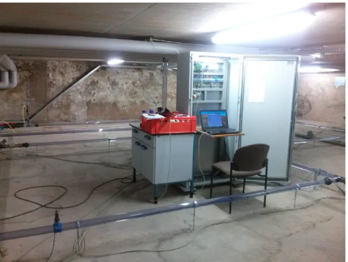
Figure 5:”Control room (SCADA System)” of the test network ... 9

Figure 6: SIR 3S signal model of Dresden test network for network operations ... 10

Figure 7: Demand modelling in the physical model ... 11

Figure 8: Pressure measurements at nodes pressure 1 and pressure 2... 12

Figure 9: Flow measurements Z1 – Z4. ... 12

Figure 10: Flow measurements Z5 – Z8. ... 13

Figure 11: Incomplete mixing at pipe cross ... 14

Figure 12: Double-T-junction (left) and two T-junctions with valves (right) ... 14

Figure 13: Contamination front (blue tracer colour) ... 15

Figure 14: SIR 3S source identification results for Dresden test network after first alarm ... 16

Figure 15: SIR 3S source identification results after first positive and second negative alarm ... 16

Figure 16: Result of Source Identification (live presentation March, 18, 2015) ... 17

Figure 17: TZW network and velocity ... 18

Figure 18: Comparison between transport model and 3 experimentations at 7h, 10h, 11h ... 18

Figure 19: Comparison between dispersion model (laminar profile) and experimentations (7h, 10h, 11h) ... 19

Figure 20: Comparison between dispersion model (mix laminar profile and average velocity, 40%/60%) and experimentations (7h, 10h, 11h) ... 20

Figure 21: Dimensions of the network and exact location of pipes ... 21

Figure 22: Closed valves and resulting flow directions ... 22

List of Tables: Table 1: Reynolds variation for different pathways for the three experiments ... 20

(6)

Testing and optimisation of online simulation model for a miniaturised distribution network 31 March 2015 5 Contents: 1 Introduction ... 6 2 Network configuration ... 6

2.1 SIR 3S Online model of test network ... 6

2.2 Network Characteristics: ... 7

2.3 Sir 3S Online Model... 9

2.4 Signal model: ... 10

2.5 Modelling demands in the real physical system ... 11

2.6 Model Calibration ... 12

3 Results ... 14

3.1 Incomplete Mixing... 14

3.2 Testing of Source Identification module, transport and alarm generation ... 15

3.3 Results Irstea ... 18

(7)

6

1 Introduction

For the performance of WP 5 and also WP 6 the Dresden test network was used. The communication between the different software packages via OPC was checked as well as the performance and functionality of different algorithms and models including the alarm generation module, transport and source identification calculations.

2 Network configuration

2.1 SIR 3S Online model of test network

The SIR 3S model of the test network in Dresden is shown in Figure 1. There is one input node (pressure 1) where the water enters the system. Three demand nodes are modelled and equipped

Figure 1: SIR 3S model of Dresden test network

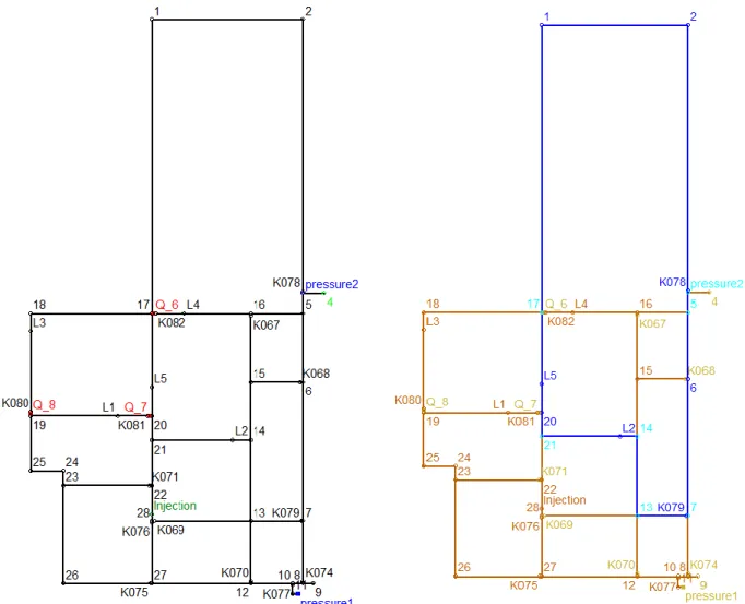
with flow meters (Z6, Z7, Z8). For flushing purposes of the pipes there is also an additional outlet node (pressure 2). Figure 2 shows again the network including the IDs of the junctions that

(8)

7

were used in the SIR 3S model. For better orientation the same IDs are also used in the photographs of the test network that are shown in the following sections of this document.

Figure 2: Node IDs of test network (left) and results of graph decomposition (right)

2.2 Network Characteristics:

- Length of all pipes sum up to 133 m

- Inner diameter of all pipes 57 mm, assumed roughness set to 0.1 mm.

- All 9 valves are closed resulting in the network topology with one loop only (blue links in Figure 2)

- The location of the measurement of Pressure1 is the inflow into the system - Pressure 2 (at the outflow) is an additional pressure measurement

- Z6 / Z7 / Z8 are locations of demand

- Flow meters (Z1 – Z5) in Figure 1 indicate location of velocity measurement

- Locations of conductivity measurements (L1 to L5) were changed for different test cases. Figure 3 gives an overview of the test network in the lab.

(9)

8

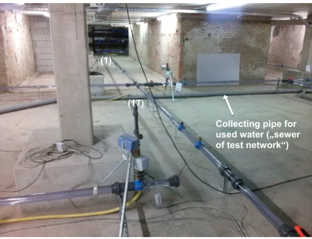
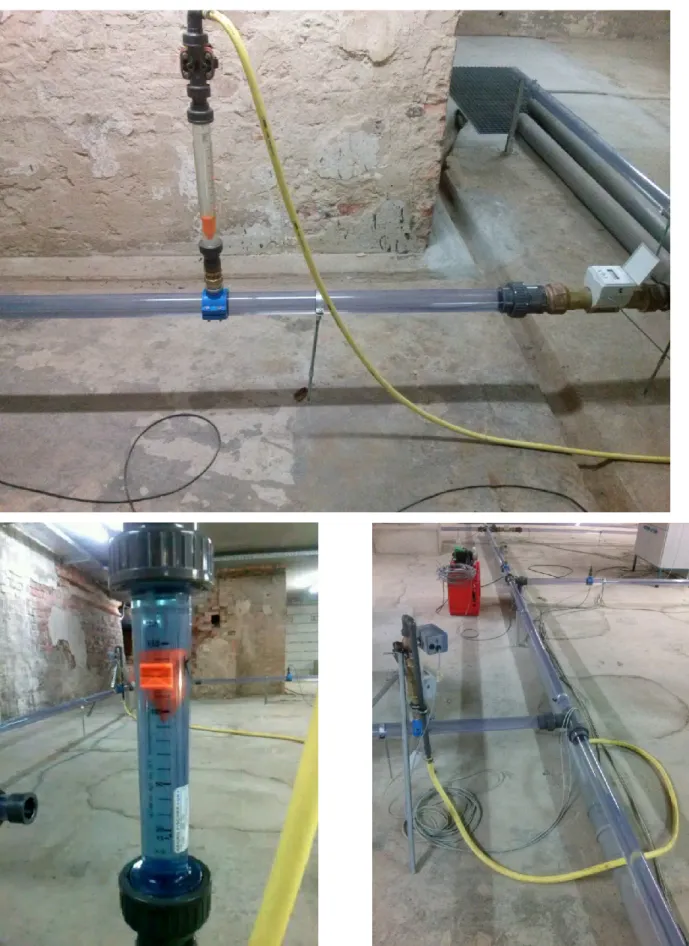
Figure 3: Configuration of Dresden test network

Figure 4: Outflow pipe for flushing of network

Collecting pipe for used water („sewer of test network“) (17) (1) closed valves (5) (2) outflow

(10)

9

2.3 Sir 3S Online Model

The values of the measurements of flows/velocities (Z1 – Z5), demands (Z6 – Z8), pressures at nodes pressure 1 and pressure 2 as well as the electrical conductivity of the water at locations L1 to L5 are transferred via cable connections to a central operating and monitoring unit (SPS) that includes an OPC Server (Panasonic). From the OPC server the data can be transferred to the hydraulic calculations using the OPC client SIR OPC that has been developed partly during the project by 3S. The OPC client is the central unit that maps data between different software components including hydraulic simulation, alarm generation and source identification. For more details on the online client SIR OPC please refer to D 5.2 of the SMaRT-OnlineWDN project. Comment on velocity measurement:

Velocity is determined by Flow measurements. These flow meters are of a smaller Di = 50 mm compared to the pipes Di = 57 mm. This value is converted into velocity and then transferred to the OPC Server.

(11)

10

2.4 Signal model:

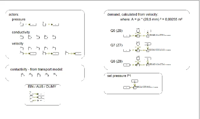
For modeling of the network operations a SIR 3S signal model has been implemented (Figure 6). The signal model receives the online data from SIR OPC and the simulation model. Some of the measurements are used as boundary conditions (actors) and the rest is used for comparison of calculation results. The comparison is important for model calibration at the beginning. Later on the delta values give a good overview over the quality of the simulation results or it can be used for online calibration (D 5.4).

On the left side in Figure 6 is the interface between hydraulic model and data (via OPC). Here the measurements of the experiment as well as the results from the transport model are inserted into the model. On the right side the measurements are directed to their equivalent element in the model – in case they set a boundary condition. The demand is calculated from the velocity measurement.

(12)

11

2.5 Modelling demands in the real physical system

(13)

12

The demands were modelled by configurable withdrawal equipment that enable the definition of certain outflow. The water is let by the yellow tube to a central collecting pipe.

2.6 Model Calibration

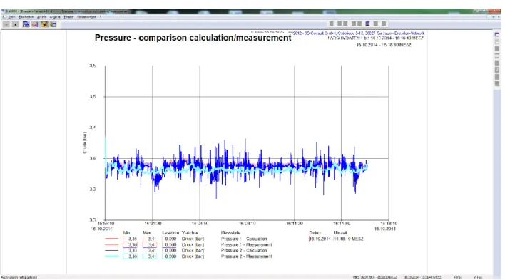
Figure 8: Pressure measurements at nodes pressure 1 and pressure 2

For model calibration the online measurements were presented as time series plots in the software Sir MMK. The software automatically updates if new data is available from the OPC server and plots the time series of different configurable values. Especially the comparison of calculated values versus measurements is useful for network calibration.

(14)

13

Due to the small extension of the network and the low roughness values of the plastic pipes there were only very small head losses in the system (Figure 8).

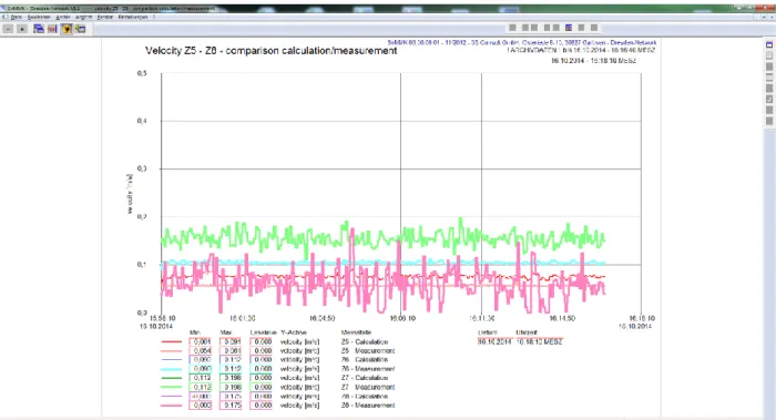
Figure 10: Flow measurements Z5 – Z8.

In order to get clear hydraulic conditions a number of valves was closed for the experiments as explained above. The only remaining loop is shown in Figure 2 (blue coloured pipes).

The time series plots in Figure 9 and Figure 10 show an early state of the calibration where the flow velocities at Z2 and Z5 differ from the measurements (see for example the light blue and dark blue curves for Z2 in Figure 9). From the network topology it is clear that Z4 = Z2 + Z5. The calculated value of the velocity (moving average) of Z5 exceeds the measurements by the same value as the measurements of Z2 exceed the corresponding calculated value. That means that the hydraulic resistance between Z4 and junction 5 must be increased. Please note that the head loss is not only a result of friction along the pipe wall but also includes the local minor losses caused by fittings and bends.

(15)

14

3 Results

3.1 Incomplete Mixing

The test network was used for different purposes. First, the incomplete mixing for different flow regimes was studied and compared with calculation results of the CFD simulations of WP 4. Therefore different combinations of pipe crosses and Double T-junctions (Figure 12) were used.

Figure 11: Incomplete mixing at pipe cross

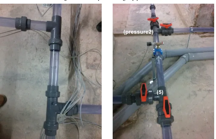
Figure 12: Double-T-junction (left) and two T-junctions with valves (right)

(5) (pressure2)

(16)

15

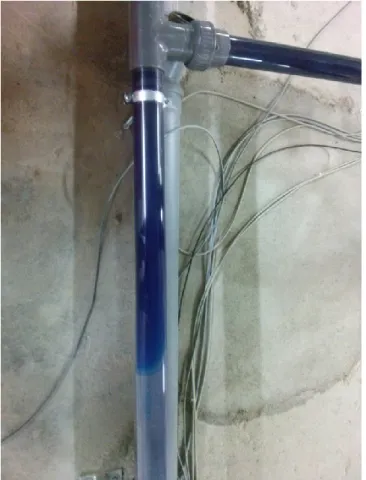
For the performance of WP 5 the laboratory network was used for proofing the entire SMaRT-OnlineWDN system functionality including hydraulic simulation, transport, alarm generation, source identification and look ahead simulations with response. For that purpose a “contamination” scenario represented by an injection of a salty solution and a colour tracer was processed. The spread of contamination could be followed visually by the tracer Figure 13.

Figure 13: Contamination front (blue tracer colour)

3.2 Testing of Source Identification module, transport and alarm generation

The comprehensive system performance included the requirement that the communication between the different software components worked properly. For that purpose a number of field tests have been carried out by 3S and IOSB. At the final presentation of the project on March 18th a similar field test was presented to the audience. The scenario includes the injection of a contaminant and the release of alarms by the alarm generation module for all five water quality sensors.

Figure 14 shows the expected result after the first alarm (red circle). The red lines are the possible locations of the source and the yellow lines are the look ahead spread of contamination. In Figure 15 there is also the signal of negative sensor alarm (light green) considered. As a result, the set of candidate locations for the source is decreased. In Figure 16 the final result of the live presentation is shown after the contamination reached all five conductivity sensors.

(17)

16

Figure 14: SIR 3S source identification results for Dresden test network after first alarm

(18)

17

(19)

18

3.3 Results Irstea

Some experiments have been done on the TZW experimental water network concerning

calibration of velocity by measuring conductivity of a chemical product injected in the network.

Figure 17: TZW network and velocity

On Figure 17 is shown the experimental network with the length given for each pipe. Conductivity sensors have been fixed at points L1, L2, L3, L4 and L5. The injection of contaminant is done at the point “House” (middle right), a constant profile injected at 60s during 120s. The water comes from the resource “In” and ends at demand points L1, L3 and L5. Flow meters are placed in such a way that all pipe flows are known (see Table 1). Simulations have been done with 1mg/L injected at “House”. It was necessary to scale the results of the simulation to correspond to the experiment. From the simulation we get concentration in mg/L and from the experiments it is conductivity. Both are assumed proportional and we calculate the coefficient of proportionality by the experimental result area under the curve (integral).

(20)

19

Experiments and calculations have been compared, the Figure 18 shows the results under three different hydraulic permanent states (7h, 11h and 10h). For simulations, the entry profile is simply transported. For experiments, the profile is stretched and reaches sensors earlier than simulated. This must be the phenomenon of dispersion, the velocity profile on the cross section of the pipe should be taken into account. Indeed, at least for laminar case, velocity at the centre of the tube is bigger than near the wall. Therefore some contaminant parts are in advance when others are late compared to average velocity.

The Figure 19 has been obtained using a laminar velocity profile for all pipes. A model of particle backtracking has been used along the cross-section to take into account the different velocities. They are launched at the end of the pipe at time t1 and when reaching the beginning of the pipe at time t0, by backtracking, they recover the concentration value. If the transport is without reaction, that value is the one that is put at the node end of the pipe at time t1. All particle launched are then integrated along the cross section to have the average concentration.

Figure 19: Comparison between dispersion model (laminar profile) and experimentations (7h, 10h,

11h)

The dispersion model gives better matching with experiments concerning the reaching time at all nodes. However, the shape doesn’t correspond with the experiments, the simulations results, when adding dispersion effect, are more spread. This might be due to the fact that a laminar profile has been used for all pipes when the Reynolds is also above 2 000 (see Table 1).

(21)

20

Table 1: Reynolds variation for different pathways for the three experiments

Pathway Dxf11->L3 Dxf28->L5 Dxf16->Dxf11 House->Dxf16 Dxf16->Dxf28 Dxf11->Dxf28

Length [m] 6.57 5.59 6.00 3.50 20.84 34.93

Reynolds 7h 942 2 505 2 505 3 847 1 327 1 578

Reynolds 10h 2 715 8 161 7 072 10 876 3 783 4 481

Reynolds 11h 3 352 5 409 6 413 8 761 2 385 3 024

Figure 20: Comparison between dispersion model (mix laminar profile and average velocity,

40%/60%) and experimentations (7h, 10h, 11h)

Figure 20 shows the result of the simulation when the profile on the cross section of the pipe is a combination between a laminar profile (40%) and the average velocity (60%). The results better match for the shape, indicating that the difference may be due of the velocity profiles not being well modelled. It might depend on the average velocity as well as the geometry in the network. Still, average velocities don’t match. Indeed, no matter the profiles used, the peak of concentration always happens the same time, it corresponds to the average velocity and the middle of the input profile of concentration. This may be due to the conductimeters being at the centre of the pipe (where the velocity is bigger).

The experiments show the existence of the dispersion phenomena on laminar and turbulent regimes. A model based on particle backtracking has been proposed to improve the predictions. It depends on the goodness-of-fit of hydraulics. The difference remaining might be due the sensors being at the centre of the tubes, where the velocity is bigger.

(22)

21

4 Appendix: Network map

(23)

22