Publisher’s version / Version de l'éditeur:
https://publications-cnrc.canada.ca/fra/droits
L’accès à ce site Web et l’utilisation de son contenu sont assujettis aux conditions présentées dans le site LISEZ CES CONDITIONS ATTENTIVEMENT AVANT D’UTILISER CE SITE WEB.
Research Report (National Research Council of Canada. Institute for Research in Construction), 2006-08-09
READ THESE TERMS AND CONDITIONS CAREFULLY BEFORE USING THIS WEBSITE.
https://nrc-publications.canada.ca/eng/copyright
NRC Publications Archive Record / Notice des Archives des publications du CNRC :
https://nrc-publications.canada.ca/eng/view/object/?id=99e27d8c-826f-422a-aa42-53b8e6ed6bce https://publications-cnrc.canada.ca/fra/voir/objet/?id=99e27d8c-826f-422a-aa42-53b8e6ed6bce
NRC Publications Archive
Archives des publications du CNRC
For the publisher’s version, please access the DOI link below./ Pour consulter la version de l’éditeur, utilisez le lien DOI ci-dessous.
https://doi.org/10.4224/20377775
Access and use of this website and the material on it are subject to the Terms and Conditions set forth at
Detection of Localized Sound Leaks or "Hot Spots" and their Effects on Architectural Speech Privacy (Speech Security)
http://irc.nrc-cnrc.gc.ca
Detection of Localized Sound Leaks or “Hot Spots” and Their
Effects on Architectural Speech Privacy (Speech Security)
I R C - R R - 2 2 4
G o v e r , B . N . ; B r a d l e y , J . S .
Detection of Localized Sound Leaks or “Hot Spots” and their
Effects on Architectural Speech Privacy (Speech Security)
Acknowledgements
This project was jointly funded by Public Works and Government Services Canada (PWGSC), the Royal Canadian Mounted Police (RCMP), and the National Research Council (NRC).
Summary
Recent projects at IRC have resulted in the development of a new measurement procedure for rating the architectural speech privacy (speech security) of a closed room. For a test sound field, the level differences between average levels within the closed room and received levels at spot locations near the walls and boundaries on the outside the room are determined. By measuring at individual receiving locations, the procedure is capable of evaluating localized sound leaks or “hot spots” without any additional effort, as all receiving locations are tested in the same manner. If sound leak locations are known or suspected, they can be tested. On the other hand, an unknown or unexpected leak may be revealed by the results of the procedure.
This report summarizes measurements made on a test wall that was modified to include a variety of defects. The severity and detectability of the known defects was investigated. Not all defects were severe enough to cause a leak that was any worse than the natural variation of sound insulation across the wall. Other defects were marginally severe enough to affect the speech privacy rating. These types of defects were, in general, not detectable with conventional measurements of transmission loss, but were detectable with the new speech privacy measurement procedure. More serious and obvious defects were also readily detectable with the new procedure.
Additionally, a new approach seeking to quickly identify sound leak locations with a directional microphone array has been investigated. For the less-significant sound leaks, this approach yielded results that require some interpretation—the presence and location of the leaks were detectable, but not obviously so. For the more obvious and serious sound leaks, the microphone array measurements yielded excellent results: the locations of the sound leaks were quickly and accurately identified.
This report first summarizes the new speech privacy measurement technique, and the test wall measurement approach. The detectability and severity of several types of intentionally introduced wall defects are discussed, measured with both conventional transmission loss tests, and with the new approach. The effect of each defect on the speech privacy risk is discussed. Lastly, the leak detection efforts with the microphone array are presented. The results are summarized in the concluding section, and, for reference, the Appendix contains the relevant spot location level difference data for all the wall configurations.
The results of the investigations indicate: that the new speech privacy measurement procedure is capable of identifying and rating a range of sound leaks; that not all wall defects are severe enough to constitute a leak affecting the speech privacy rating; and that the idea of using a directional microphone array as a quick leak detector, while not without its limitations, is nonetheless viable in some situations.
Contents
Acknowledgements... 2
Summary ... 3
Contents ... 4
1. Introduction... 5
2. Investigating Localized Sound Leaks or “Hot Spots” ... 6
2.1. Overview of Speech Privacy Measurement Procedure... 6
2.2. Laboratory Measurements on Test Wall... 8
3. Characterization of Wall Defects... 11
3.1. No Intentional Leaks... 12
3.2. Penetrations... 14
3.2.1. 2.5 cm diameter hole... 14
3.2.2. 5.4 cm diameter hole... 16
3.2.3. 3.8 cm diameter pipe through 5.4 cm diameter hole... 18
3.3. Electrical Boxes ... 20
3.3.1. One box... 20
3.3.2. Two boxes: back-to-back... 22
3.3.3. Two boxes: offset... 24
3.3.4. Two boxes: wide offset, one in stud cavity with no absorptive batts ... 26
3.4. Holes in One Side of Wall Only ... 28
3.4.1. 15-by-15 cm hole ... 28
3.4.2. 20-by-20 cm hole ... 30
3.5. One Stud Cavity with No Absorptive Batts... 32
3.5.1. No holes in drywall... 32
3.5.2. 15-by-15 cm hole in one side: no absorption... 34
3.5.3. 20-by-20 cm hole in one side: no absorption... 36
3.6. Summary of Wall Defect Characterization... 38
4. Array-Based Detection of Hot Spots ... 39
4.1. No Intentional leaks ... 43
4.2. Hole in One Side... 45
4.3. Penetrations... 46
4.3.1. 5.4 cm diameter hole... 46
4.3.2. 3.8 cm diameter pipe through 5.4 cm diameter hole... 47
4.4. Electrical Boxes ... 48
4.4.1. Two boxes: back-to-back... 48
4.4.2. Two boxes: offset... 48
4.5. Summary of Array-Based Detection Measurements ... 49
5. Conclusions... 51
References... 52
1. Introduction
Speech privacy is a concern for closed offices and meeting rooms, when conversations occurring within are intended to be difficult to hear or to understand outside the room. The degree to which the speech transmitted from within a room to listening positions in the adjoining spaces is intelligible or audible depends on the sound insulation provided by the building. Since the sound insulation can be expected to vary from point-to-point, then so too can the degree of speech privacy. This report addresses the issue of point-to-point variation of sound insulation; in particular, the presence and effect of localized weak spots. Such weak spots in the insulation could be considered a sound leak or “hot spot”, resulting in a greatly reduced speech privacy rating at that location.
The term speech privacy is used to describe the degree to which overhead speech is difficult to hear or understand. Speech security is used for the discussion of very high levels of privacy, and typically in situations where the building users need to guarantee a minimum (high) level of privacy. Discussion of architectural speech privacy or security limits the scope to privacy due to the building and building services, and to live listening without the use of electroacoustic listening devices (such as microphones, recorders, etc.).
In situations where building users have performance criteria, the idea is that if an adequate level of privacy can be assured, then the conditions may be said to be speech secure. When qualifying a room as adequately private or secure, it must be ensured that sufficient insulation is provided at all potential eavesdropping locations. This means that the presence of localized sound leaks must be considered, as the room may be only as good as its weakest point.
Recent investigations at IRC have developed a framework and procedures for predicting and rating the architectural speech privacy (speech security) of meeting rooms and closed offices [1]. One part of this work is a field measurement procedure for evaluating existing rooms [2]. The measurement protocol treats listening locations near sound leaks in exactly the same manner as all other locations—the results indicate whether or not there is reduced speech privacy. Part of the problem then becomes to understand what constitutes a sound leak, and where to look for them.
This report presents the results of investigations characterizing the detectability and severity of several types of sound leaks introduced into a test wall. Section 2 presents a review of the new speech privacy measurement procedure, and descriptions of the testing facility and of the measurements. The measurement results are shown in Section 3 for a variety of leaks, including penetrations, electrical boxes, and holes. Section 4 contains results from efforts using a directional microphone array as quick detector of leaks in the wall. Section 5 presents the summary and conclusions. An appendix to this report contains
2. Investigating Localized Sound Leaks or “Hot Spots”
The degree of speech privacy depends on the reduction of speech levels upon transmission from within the room to a particular listening point outside the room. Less sound reduction implies less privacy, and vice versa. From point to point, some natural variation of sound insulation (and therefore degree of privacy) is to be expected, but in addition, there will be problems near defects and peculiarities such as electrical boxes, pipe penetrations, holes, etc. If the sound insulation is compromised to an extent that affects the privacy rating, then the localized sound leak is of concern. Section 2.1 reviews the new speech privacy measurement procedure, and Section 2.2 describes the current measurements.2.1. Overview of Speech Privacy Measurement Procedure
The newly developed measurement procedure [1,2] determines the degree of speech privacy from within a closed room to individual spot locations outside the room. This is illustrated schematically in Figure 1, showing the sound source inside the room to be tested, and microphone positions both in the room with the source, and at each receiving location to be considered. Typically, receiving locations are selected a distance of 0.25 m from the boundary of the room, as well as at any other location of interest (such as a suspected sound leak).
Figure 1 Schematic diagram showing the source and microphone locations in the room under test, and spot receiving locations in the adjoining spaces. The spot receiver locations are typically 0.25 m from the boundaries of the room, and at the locations of any suspected sound leaks.
The omnidirectional source in the source room is used to play high levels of steady-state white noise. While the noise is playing, the one-third-octave band sound pressure levels are measured at points throughout the source room (but away from the source and the walls), and also at each receiving location. This is repeated for at least one other source position. The measurements are used to calculate the average source room levels, LS(f),
and the receiving point levels, LR(f), in each one-third-octave band centred at frequency f,
from 160 to 5000 Hz. These are used to calculate the level differences
) ( ) ( ) ( f R L f S L f LD = − , (1)
which describe the sound insulation from an average, uniform sound field in the source room to each listening position. These level differences can be used to calculate the Speech Privacy Index (SPI) [1,3], given by
[
]
32 5 160 ) ( ) ( ) ( 16 1 − =∑
− − = kHz Hz f f N f LD f S SPI , (2)where in each one-third-octave band centred at frequency f, S(f) is the level of source room
speech and N(f) is the level of receiving point background noise. The subscript –32 means
that the quantity in square brackets should be clipped to have a minimum value of –32 dB.
To calculate SPI using Eq. (2), an assumed speech spectrum and noise spectrum are
required. By selecting speech and noise levels that occur with a known probability [4], the resulting SPI will occur with the same probability. That is, if the speech and noise levels
used occur only 1% of the time, then the SPI value that results will also occur (i.e., be
exceeded) 1% of the time. The actual value of SPI can be compared to the threshold values
of –16 dB (threshold of intelligibility) or –22 dB (threshold of audibility) [3].
Alternatively, the measured level differences can be used directly to assess the privacy risk category. This approach is based on a simplified version of Eq. (2), assuming that the –32 dB clipping can be ignored. In this case, Eq. (2) can be re-written as
) ( ) ( )
(avg LD avg N avg
S SPI = − − , (3) or SPI avg LD avg N avg S( )− ( )= ( )+ , (4)
where (avg) indicates the arithmetic average of the one-third-octave levels from 160 to
5000 Hz. The speech and noise quantities on the left-hand side of Eq. (4) are statistical and occur with certain probabilities. The quantity on the right-hand side includes the measured
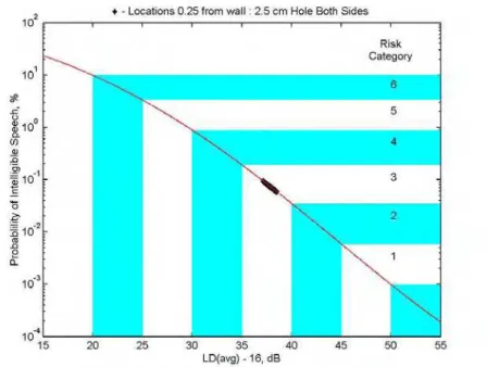
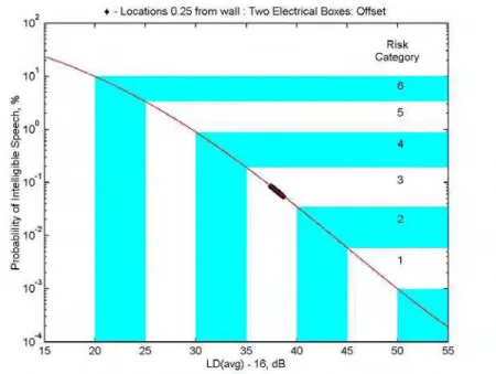
Figure 2 Probability of transmitted speech being intelligible versus LD(avg)–16 dB. The probabilities are derived assuming equally likely speech and noise levels [4].
The horizontal axis of Figure 2 is LD(avg)–16 dB, which is the arithmetic average of the
measured one-third-octave band level differences, plus –16 dB, which is the value of SPI
for the threshold of intelligibility. The key point is that the measured values of the level differences can be used to assess the risk of speech being intelligible at the listening position. The level differences will vary from point-to-point, and be smaller near sound leaks, implying a higher risk of a privacy lapse.
2.2. Laboratory Measurements on Test Wall
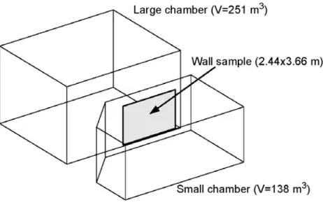
A test wall was constructed in the reverberation chamber suite in Building M-27 at NRC. This facility consists of a pair of reverberation rooms with a 2.66-by-3.44 m opening between them, into which test wall samples are constructed. A schematic is shown in Figure 3.
Figure 3 Schematic drawing of reverberation chamber test facility at Building M-27, NRC.
The wall constructed for these studies consisted of 2 layers of 16 mm drywall mounted on both sides of 90 mm lightweight steel studs (406 mm on centre). The cavities of the stud spaces were filled with 90 mm mineral fibre batts. A schematic cross-section of the wall is shown in Figure 4.
After the wall was constructed, various modifications were made to intentionally introduce defects and potential sound leaks. Following each modification, for each configuration of the wall, measurements were made to characterize the sound transmission and assess the effect of the leak. The measurements for each configuration included:
1. A standard ASTM E90 transmission loss test [5]. This test measures the one-third-octave band level differences between average, uniform levels in the source room and in the receiving room. This is different from the new speech privacy measurement protocol in that the receiving side measurements are made in the interior of the receiving room, away from the wall. The results yield information on the average sound insulation of the wall, but no information on point-to-point variation of that performance. The transmission loss is used to derive the Sound Transmission Class (STC) rating of the wall, which is a commonly-cited single-number indicator.
2. Steady-state (30-second average) measurements of the one-third-octave band levels in the source room and at locations 0.25 m from the wall in the receiving room. The level difference from source room average to spot receiver, LD(f), is obtained. This is essentially the new speech privacy
measurement protocol. Four conventional loudspeakers driven simultaneously and independently were used to establish the test sound field. A grid of 63 (7x9) positions 0.25 m from the surface of the wall was used for receiving positions. The positions were regularly spaced 0.45 m horizontally, and 0.38 m vertically.
3. Impulse response measurements from a single, omnidirectional source located in the source room to a highly directional microphone array, located 1.05 m from the wall in the receiving room. An impulse response shows the sound pressure arriving at the receiving point versus time, after the emission of a pulse by the source. This gives information on the temporal nature of the sound transmission through the wall, and throughout the receiving space. Furthermore, the array is capable of discriminating sound arriving from different directions. Directions of peak sound incidence can potentially be traced back to the wall, and sound leaks identified.
4. Impulse response measurements from a single, omnidirectional source located in the source room to the grid of 0.25 m receiving positions. These show the time evolution of the sound field near the wall.
The results of the first two types of measurements (ASTM E90 and new speech privacy approach) are discussed in Section 3 below, for each of the configurations of the wall. The array and impulse response measurements were more exploratory, and are discussed in Section 4.
3. Characterization of Wall Defects
This section presents the results of the conventional ASTM E90 test and of the new speech privacy measurement spot receiver location procedure for each configuration of the test wall. The E90 test yielded the transmission loss in each one-third-octave band, which was used to obtain the STC. The new speech privacy measurement procedure yielded the level differences LD(f) in each one-third-octave band. The arithmetic average from 160 to 5000
Hz was taken to obtain LD(avg), which as shown in Figure 2, can indicate the degree of
privacy.
The following subsections present the results for the following configurations of the wall:
1. No Intentional Leaks 2. Penetrations
2.1. 2.5 cm diameter hole 2.2. 5.4 cm diameter hole
2.3. 3.8 cm diameter pipe through 5.4 cm hole 3. Electrical Boxes
3.1. One box
3.2. Two boxes: back-to-back 3.3. Two boxes: offset
3.4. Two boxes: wide offset, one in stud cavity with no absorptive batts 4. Holes in One Side of Wall Only
4.1. 15-by-15 cm hole 4.2. 20-by-20 cm hole
5. One Stud Cavity with No Absorptive Batts 5.1. No holes in drywall
5.2. 15-by-15 cm hole in one side 5.3. 20-by-20 cm hole in one side
The results for each configuration are discussed along with the case “No Intentional Leaks” (Section 3.1), which is the baseline measurement of the wall. Should the reader wish to skip over the details contained in the following sections, a summary of the results of these measurements is given in Section 3.6.
3.1. No Intentional Leaks
Figure 5(a) shows a drawing of the configuration of the wall, with no intentional leaks or defects. Figure 5(b) shows the transmission loss versus frequency result of the ASTM E90 test. The STC rating of the wall was 56.
(a) (b)
Figure 5 No intentional leaks: (a) wall configuration, (b) transmission loss versus frequency.
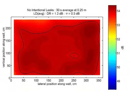
A plot of the measured LD(avg) over the surface of the wall is shown in Figure 6. The 63
measured values were used to interpolate over the whole surface. The colourmap indicates the value of LD(avg) in decibels, the peak value corresponding to the top of the colour
scale (the deepest red). The graphing procedure adds a contour line at every integer decibel. On this plot, only the 54 dB contour is present since no values were greater than 55 dB or lower than 53 dB. The difference between maximum and minimum measured values is termed the dynamic range, and was DR = 1.2 dB. The standard deviation was σ =
0.3 dB. These amounts of variation can be taken as natural, baseline deviations. From qualitative inspection of the plot, no obvious features are apparent, which is in agreement with the small quantitative variations.
Figure 7 repeats Figure 2, but overlaid are 63 data points (♦) corresponding to the measured values of LD(avg). It can be seen that there is a spread of DR = 1.2 dB, and at all
Figure 6 No intentional leaks: LD(avg) at locations 0.25 m from the wall. The 54 dB contour is shown.
Figure 7 No intentional leaks: Risk categories for intelligible speech, showing measured data points (♦). Spread of values is 1.2 dB.
3.2. Penetrations
3.2.1. 2.5 cm diameter hole
A 2.5 cm diameter hole was drilled entirely through the wall at one location about halfway between two studs. The absorptive material was not removed from the stud cavity; it blocked the line of sight through the hole. Figure 8(a) shows a drawing of the configuration of the wall. Figure 8(b) shows the transmission loss versus frequency for this configuration (STC 56) and for the “No Intentional Leaks” case (STC 56). The TL curves
are nearly identical and, in both cases, the STC rating was 56. The hole drilled in the wall is undetectable by the conventional transmission loss test and makes no difference to the STC rating.
(a) (b)
Figure 8 2.5 cm diameter hole: (a) wall configuration, (b) transmission loss versus frequency, showing ‘No Intentional Leaks’ case for comparison.
A plot of the measured LD(avg) over the surface of the wall is shown in Figure 9. Overlaid
on the plot is a white square indicating the location of the penetration (lateral position 270 cm, vertical position 75 cm). The dynamic range was DR = 1.3 dB, and the standard deviation was σ = 0.3 dB. These are essentially the same as for the “No Intentional Leaks” case (DR = 1.2 dB, σ = 0.3 dB). Qualitatively, the plot also looks very similar to the “No Intentional Leaks” case. (The penetration is in fact detectable by examining some of the individual one-third-octave band data shown in the Appendix, but has a negligible effect on the frequency-average, LD(avg).)
Figure 10 again repeats Figure 2, and overlaid are 63 data points (♦) corresponding to the measured values of LD(avg) for this case. The range of DR = 1.3 dB is evident, and at all
measured locations, the risk category for intelligible speech is Category #3, as it was for the “No Intentional Leaks” case.
It is perhaps somewhat surprising that the small hole has no significant effect on the measured LD(avg) and therefore the speech privacy, even in its immediate proximity.
Figure 9 2.5 cm diameter hole: LD(avg) at locations 0.25 m from the wall. The white square indicates the location of the penetration. The 54 dB contour is shown.
Figure 10 2.5 cm diameter hole: Risk categories for intelligible speech, showing measured data points (♦). Spread of values is 1.3 dB.
3.2.2. 5.4 cm diameter hole
The hole in the wall was enlarged to 5.4 cm in diameter. The absorptive material was not removed from the stud cavity; it blocked the line of sight through the hole. Figure 11(a) shows a drawing of the configuration of the wall. Figure 11(b) shows the transmission loss versus frequency for this configuration (STC 53) and for the “No Intentional Leaks” case (STC 56). The transmission loss curves are quite different, and the STC has changed by 3 points. The hole drilled in the wall clearly has an effect detectable by the conventional transmission loss test.
(a) (b)
Figure 11 5.4 cm diameter hole: (a) wall configuration, (b) transmission loss versus frequency, showing ‘No Intentional Leaks’ case for comparison.
A plot of the measured LD(avg) over the surface of the wall is shown in Figure 12.
Overlaid on the plot is a white square indicating the location of the penetration (lateral position 270 cm, vertical position 75 cm). A contour line is shown at every integer decibel. The dynamic range was DR = 4.8 dB, and the standard deviation was σ = 0.9 dB. These are much higher than for the “No Intentional Leaks” case. Qualitatively, the plot also looks very different—the penetration is obvious from the location of the minimum in LD(avg).
Figure 13 again repeats Figure 2, and overlaid are 63 data points (♦) corresponding to the measured values of LD(avg) for this case. The range of DR = 4.8 dB is evident, and at all
measured locations, the risk category for intelligible speech is Category #4. At some locations (close to the penetration), the category is nearly #5. Not only is the wall much worse near the penetration, but the overall performance is degraded everywhere.
Figure 12 5.4 cm diameter hole: LD(avg) at locations 0.25 m from the wall. The white square indicates the location of the penetration. Contour lines are drawn every decibel.
Figure 13 5.4 cm diameter hole: Risk categories for intelligible speech, showing measured data points (♦). Spread of values is 4.8 dB.
3.2.3. 3.8 cm diameter pipe through 5.4 cm diameter hole
A length of 3.8 cm diameter metal pipe was filled with foam, the ends plugged, and was inserted through the 5.4 cm diameter hole in the wall. The pipe was not touching the drywall. The absorptive material was not removed from the stud cavity; the pipe was passed through it. Figure 14(a) shows a drawing of the configuration of the wall. Figure 14(b) shows the transmission loss versus frequency for this configuration (STC 56) and for the “No Intentional Leaks” case (STC 56). The transmission loss curves are quite similar—the current case only lower by 1–2 decibels at some frequencies. The STC values were the same. The pipe passed through the wall is essentially undetectable by the conventional transmission loss test, and makes no difference to the STC rating.
(a) (b)
Figure 14 3.8 cm diameter pipe through 5.4 cm diameter hole: (a) wall configuration, (b) transmission loss versus frequency, showing ‘No Intentional Leaks’ case for comparison.
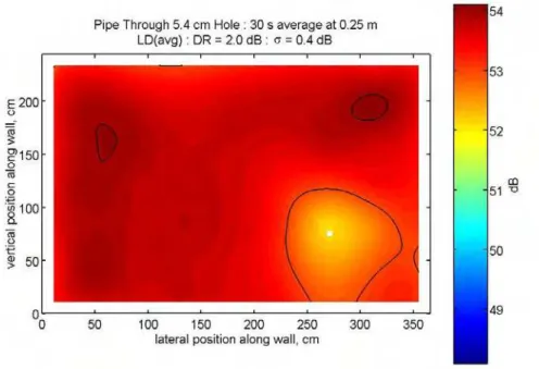
A plot of the measured LD(avg) over the surface of the wall is shown in Figure 15.
Overlaid on the plot is a white square indicating the location of the penetration (lateral position 270 cm, vertical position 75 cm). The 53 dB and 54 dB contour lines are shown. The dynamic range was DR = 2.0 dB, and the standard deviation was σ = 0.4 dB. These are slightly higher than for the “No Intentional Leaks” case. Qualitatively, the plot looks very different—the penetration is obvious from the location of the minimum in LD(avg).
Figure 16 again repeats Figure 2, and overlaid are 63 data points (♦) corresponding to the measured values of LD(avg) for this case. The range of DR = 2.0 dB is evident, and at all
measured locations, the risk category for intelligible speech is Category #3. At some locations (close to the penetration), the category is nearly #4. The wall is slightly worse near the penetration, but the overall performance is very similar to before the defect was introduced. This is also perhaps somewhat surprising.
Figure 15 3.8 cm diameter pipe through 5.4 cm diameter hole: LD(avg) at locations 0.25 m from the wall. The white square indicates the location of the penetration. The 53 dB and 54 dB contours are shown.
Figure 16 3.8 cm diameter pipe through 5.4 cm diameter hole: Risk categories for intelligible speech, showing measured data points (♦). Spread of values is 2.0 dB.
3.3. Electrical
Boxes
3.3.1. One box
All the penetrations in the wall were repaired, and a conventional duplex electrical box (face measuring 5-by-8 cm, and 6.5 cm deep) was installed on one side of the wall. The box contained two traditional grounded outlets, and was covered by a faceplate. The absorptive material was not removed from the stud cavity; the box compressed it slightly. Figure 17(a) shows a drawing of the configuration of the wall. Figure 17(b) shows the transmission loss versus frequency for this configuration (STC 56) and for the “No Intentional Leaks” case (STC 56). The curves are nearly identical and, in both cases, the STC rating was 56. The electrical box installed in the wall is undetectable by the conventional transmission loss test and makes no difference to the STC rating.
(a) (b)
Figure 17 One electrical box: (a) wall configuration, (b) transmission loss versus frequency, showing ‘No Intentional Leaks’ case for comparison.
A plot of the measured LD(avg) over the surface of the wall is shown in Figure 18.
Overlaid on the plot is a white rectangle indicating the location of the electrical box (lateral position 270 cm, vertical position 75 cm). The 54 dB contour is shown. The dynamic range was DR = 1.2 dB, and the standard deviation was σ = 0.3 dB. These are the same as for the “No Intentional Leaks” case. Qualitatively, the plot also looks very similar to the “No Intentional Leaks” case.
Figure 19 again repeats Figure 2, and overlaid are 63 data points (♦) corresponding to the measured values of LD(avg) for this case. The range of DR = 1.2 dB is evident, and at all
measured locations, the risk category for intelligible speech is Category #3, as it was for the “No Intentional Leaks” case.
Figure 18 One electrical box: LD(avg) at locations 0.25 m from the wall. The white rectangle indicates the location of the electrical box. The 54 dB contour is shown.
Figure 19 One electrical box: Risk categories for intelligible speech, showing measured data points (♦). Spread of values is 1.2 dB.
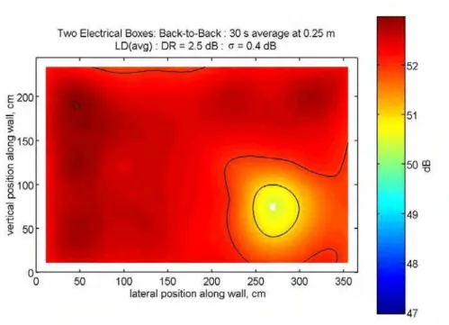
3.3.2. Two boxes: back-to-back
A second duplex electrical box (measuring 5-by-8-by-6.5 cm) was installed on the other side of the wall, immediately opposite the first box. This box also contained grounded outlets, and was covered by a faceplate. The absorptive material was not removed from the stud cavity; the boxes compressed it between them. Figure 20(a) shows a drawing of the configuration of the wall. Figure 20(b) shows the transmission loss versus frequency for this configuration (STC 55) and for the “No Intentional Leaks” case (STC 56). The curves are quite different between about 400–1600 Hz, the transmission loss being reduced by almost 10 dB at 1000 Hz. The back-to-back electrical boxes have a noticeable effect on the transmission loss, yet only a minimal effect on the STC rating.
(a) (b)
Figure 20 Two electrical boxes: back-to-back: (a) wall configuration, (b) transmission loss versus frequency, showing ‘No Intentional Leaks’ case for comparison.
A plot of the measured LD(avg) over the surface of the wall is shown in Figure 21.
Overlaid on the plot is a white rectangle indicating the location of the boxes (lateral position 270 cm, vertical position 75 cm). The 51 dB and 52 dB contours are shown. The dynamic range was DR = 2.5 dB, and the standard deviation was σ = 0.4 dB. These are higher than for the “No Intentional Leaks” case. Qualitatively, the penetration is obvious from the location of the minimum in LD(avg).
Figure 22 again repeats Figure 2, and overlaid are 63 data points (♦) corresponding to the measured values of LD(avg) for this case. The range of DR = 2.5 dB is evident. At most
measured locations, the risk category for intelligible speech is Category #3, but at some locations (close to the electrical boxes), the category is #4. The sound insulation of the wall is much worse near the back-to-back electrical boxes.
Figure 21 Two electrical boxes: back-to-back: LD(avg) at locations 0.25 m from the wall. The white rectangle indicates the location of the back-to-back electrical boxes. The 51 dB and 52 dB contours are shown.
Figure 22 Two electrical boxes: back-to-back: Risk categories for intelligible speech, showing measured data points (♦). Spread of values is 2.5 dB.
3.3.3. Two boxes: offset
One of the two electrical boxes was moved to the next stud, on the other side of the stud cavity. Both boxes were still located in the same stud cavity, but were horizontally offset by about 30 cm. The absorptive material was not removed from the stud cavity; the boxes compressed it behind them. Figure 23(a) shows a drawing of the configuration of the wall. Figure 23(b) shows the transmission loss versus frequency for this configuration (STC 56) and for the “No Intentional Leaks” case (STC 56). The curves are nearly identical, and the STC ratings are the same. The offset electrical boxes have no effect on the transmission loss.
(a) (b)
Figure 23 Two electrical boxes: offset: (a) wall configuration, (b) transmission loss versus frequency, showing ‘No Intentional Leaks’ case for comparison.
A plot of the measured LD(avg) over the surface of the wall is shown in Figure 24.
Overlaid on the plot are two white rectangles indicating the locations of the boxes (lateral position 240 cm and 270 cm, vertical positions 75 cm). The 54 dB contour is shown. The dynamic range was DR = 1.2 dB, and the standard deviation was σ = 0.3 dB. These are the same as for the “No Intentional Leaks” case. Qualitatively, no features indicating a weak spot are evident.
Figure 25 again repeats Figure 2, and overlaid are 63 data points (♦) corresponding to the measured values of LD(avg) for this case. The range of DR = 1.2 dB is evident. At all
measured locations, the risk category for intelligible speech is Category #3, just as for the “No Intentional Leaks” case. The sound insulation of the wall was not affected by the offset electrical boxes.
Figure 24 Two electrical boxes: offset: LD(avg) at locations 0.25 m from the wall. The white rectangles indicate the locations of the electrical boxes. The 54 dB contour is shown.
Figure 25 Two electrical boxes: offset: Risk categories for intelligible speech, showing measured data points (♦). Spread of values is 1.2 dB.
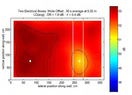
3.3.4. Two boxes: wide offset, one in stud cavity with no absorptive batts
One of the two electrical boxes was moved four stud space cavities away from the first. The boxes were horizontally offset by about 2 m. Also, the absorptive batts were removed from the stud cavity containing the first box. Figure 26(a) shows a drawing of the configuration of the wall. Figure 26(b) shows the transmission loss versus frequency for this configuration (STC 56) and for the “No Intentional Leaks” case (STC 56). The curves are different between 500-1600 Hz, the transmission loss being lower by up to 5 dB in the presence of the boxes. The STC ratings, however, were the same.
(a) (b)
Figure 26 Two electrical boxes: wide offset, one in stud cavity with no absorptive batts: (a) wall configuration, (b) transmission loss versus frequency, showing ‘No Intentional Leaks’ case for comparison.
A plot of the measured LD(avg) over the surface of the wall is shown in Figure 27.
Overlaid on the plot are two white rectangles indicating the locations of the boxes (lateral position 75 cm and 270 cm, vertical positions 75 cm), and two white vertical lines indicating the stud cavity that was empty of absorption (lateral position 245 cm and 285 cm). The 52 dB and 53 dB contours are shown. The dynamic range was DR = 1.9 dB, and the standard deviation was σ = 0.4 dB. These are slightly higher than for the “No Intentional Leaks” case (DR = 1.2 dB, σ = 0.3 dB). Qualitatively, the box installed in the stud cavity with no absorption is clearly a weak spot in the sound insulation of the wall. The other box, as expected from the results of Section 3.3.1, has no effect.
Figure 28 again repeats Figure 2, and overlaid are 63 data points (♦) corresponding to the measured values of LD(avg) for this case. The range of DR = 1.9 dB is evident. At all
measured locations, the risk category for intelligible speech is Category #3, but some locations near the box in the empty stud cavity, the category is nearly #4.
Figure 27 Two electrical boxes: wide offset, one in stud cavity with no absorptive batts:
LD(avg) at locations 0.25 m from the wall. The white rectangles indicate the locations of
the electrical boxes. The white vertical lines indicate the stud cavity with no absorption. The 52 dB and 53 dB contours are shown.
3.4. Holes in One Side of Wall Only
3.4.1. 15-by-15 cm hole
All the previous defects in the wall were repaired, and a square hole measuring 15-by-15 cm was cut through both layers of drywall on one side of the wall only, midway between two studs. The absorptive material was not removed from the stud cavity, and the other side of the wall was left intact. Figure 29(a) shows a drawing of the configuration of the wall. Figure 29(b) shows the transmission loss versus frequency for this configuration (STC 55) and for the “No Intentional Leaks” case (STC 56). The curves are very similar, the transmission loss being lower by only a few decibels at some frequencies when the hole was present. The hole in one side of the wall has a small effect on the transmission loss and makes only a one point difference to the STC rating.
(a) (b)
Figure 29 15-by-15 cm hole in one side: (a) wall configuration, (b) transmission loss versus frequency, showing ‘No Intentional Leaks’ case for comparison.
A plot of the measured LD(avg) over the surface of the wall is shown in Figure 30.
Overlaid on the plot is a white square indicating the location of the hole (lateral position 260 cm, vertical position 120 cm). The 53 dB contour is shown. The dynamic range was DR = 1.5 dB, and the standard deviation was σ = 0.4 dB. These are slightly higher than for the “No Intentional Leaks” case (DR = 1.2 dB, σ = 0.3 dB). Qualitatively, the plot looks very similar to the “No Intentional Leaks” case, but the minimum value of LD(avg) is
noticeable in the vicinity of the hole.
Figure 31 again repeats Figure 2, and overlaid are 63 data points (♦) corresponding to the measured values of LD(avg) for this case. The range of DR = 1.5 dB is evident, and at all
measured locations, the risk category for intelligible speech is Category #3, as it was for the “No Intentional Leaks” case, however the points for some locations appear to be closer to Category #4, due to the reduced sound insulation near the hole.
Figure 30 15-by-15 cm hole in one side: LD(avg) at locations 0.25 m from the wall. The white square indicates the location of the hole. The 53 dB contour is shown.
Figure 31 15-by-15 cm hole in one side: Risk categories for intelligible speech, showing measured data points (♦). Spread of values is 1.5 dB.
3.4.2. 20-by-20 cm hole
The square hole cut through both layers of drywall on one side of the wall only was enlarged to 20-by-20 cm. The absorptive material was not removed from the stud cavity, and the other side of the wall was left intact. Figure 32(a) shows a drawing of the configuration of the wall. Figure 32(b) shows the transmission loss versus frequency for this configuration (STC 55) and for the “No Intentional Leaks” case (STC 56). The curves are very similar, but the transmission loss was lower by a few decibels between 125 and 1600 Hz when the hole was present. The hole in one side of the wall has a small effect on the transmission loss and makes a one point difference to the STC rating.
(a) (b)
Figure 32 20-by-20 cm hole in one side: (a) wall configuration, (b) transmission loss versus frequency, showing ‘No Intentional Leaks’ case for comparison.
A plot of the measured LD(avg) over the surface of the wall is shown in Figure 33.
Overlaid on the plot is a white square indicating the location of the hole (lateral position 260 cm, vertical position 120 cm). The 52 dB and 53 dB contours are shown. The dynamic range was DR = 1.8 dB (slightly higher than for the “No Intentional Leaks” case DR = 1.2 dB), and the standard deviation was σ = 0.3 dB (same as for the “No Intentional Leaks” case). Qualitatively, the minimum value of LD(avg) at the location of the hole is
noticeable.
Figure 34 again repeats Figure 2, and overlaid are 63 data points (♦) corresponding to the measured values of LD(avg) for this case. The range of DR = 1.8 dB is seen, and at all
measured locations, the risk category for intelligible speech is Category #3, as it was for the “No Intentional Leaks” case, however the points for some locations appear to be closer to Category #4, due to the reduced sound insulation near the hole.
Figure 33 20-by-20 cm hole in one side: LD(avg) at locations 0.25 m from the wall. The white square indicates the location of the hole. The 52 dB and 53 dB contours are shown.
Figure 34 20-by-20 cm hole in one side: Risk categories for intelligible speech, showing measured data points (♦). Spread of values is 1.8 dB.
3.5. One Stud Cavity with No Absorptive Batts
3.5.1. No holes in drywall
All the previous defects in the wall were repaired, but the absorptive batts were removed from one of the nine stud space cavities. The absorptive material was not removed from the other eight stud cavities, and all the drywall was left intact. Figure 35(a) shows a drawing of the configuration of the wall. Figure 35(b) shows the transmission loss versus frequency for this configuration (STC 55) and for the “No Intentional Leaks” case (STC 56). The curves are very similar, the transmission loss being lower by 1–2 decibels at some frequencies when the absorption was missing. The absence of absorption has a small effect on the transmission loss and makes a one point difference to the STC rating.
(a) (b)
Figure 35 One stud cavity with no absorptive batts: (a) wall configuration, (b) transmission loss versus frequency, showing ‘No Intentional Leaks’ case for comparison.
A plot of the measured LD(avg) over the surface of the wall is shown in Figure 36.
Overlaid on the plot are two white vertical lines indicating the stud cavity that was empty of absorption (lateral position 245 cm and 285 cm). The 53 dB contour is shown. The dynamic range was DR = 1.1 dB (compared to DR = 1.2 dB for “No Intentional Leaks” case, which is essentially the same, within measurement uncertainty), and the standard deviation was σ = 0.3 dB (same as for the “No Intentional Leaks” case). Qualitatively, the reduced values of LD(avg) near the empty stud cavity are noticeable.
Figure 37 again repeats Figure 2, and overlaid are 63 data points (♦) corresponding to the measured values of LD(avg) for this case. The range of DR = 1.1 dB is evident, and at all
measured locations, the risk category for intelligible speech is Category #3, as it was for the “No Intentional Leaks” case. Removing the absorption from one stud space doesn’t greatly affect the sound insulation or the degree of speech privacy.
Figure 36 One stud cavity with no absorptive batts: LD(avg) at locations 0.25 m from the wall. The white vertical lines indicate the stud cavity with no absorption. The 53 dB contour is shown.
Figure 37 One stud cavity with no absorptive batts: Risk categories for intelligible speech, showing measured data points (♦). Spread of values is 1.1 dB.
3.5.2. 15-by-15 cm hole in one side: no absorption
A square hole measuring 15-by-15 cm was cut through both layers of drywall on one side of the wall only, into the stud space cavity that had no absorption, midway between the studs. The absorptive material was not removed from the other eight stud cavities, and the other side of the wall was left intact. Figure 38(a) shows a drawing of the configuration of the wall. Figure 38(b) shows the transmission loss versus frequency for this configuration (STC 52) and for the “No Intentional Leaks” case (STC 56). The curves are quite different, the transmission loss being lower by up to10 decibels at all frequencies above 125 Hz when the hole was present. The hole in one side of the wall and the absence of absorption had a significant effect on the transmission loss, and made a 4 point difference to the STC rating.
(a) (b)
Figure 38 One stud cavity with no absorptive batts: 15-by-15 cm hole in one side: (a) wall configuration, (b) transmission loss versus frequency, showing ‘No Intentional Leaks’ case for comparison.
A plot of the measured LD(avg) over the surface of the wall is shown in Figure 39.
Overlaid on the plot is a white square indicating the location of the hole (lateral position 260 cm, vertical position 120 cm), and two white vertical lines indicating the stud cavity that was empty of absorption (lateral position 245 cm and 285 cm). A contour is shown every decibel. The dynamic range was DR = 4.2 dB, and the standard deviation was σ = 1.1 dB. These are much higher than for the “No Intentional Leaks” case (DR = 1.2 dB, σ = 0.3 dB). Qualitatively, reduced sound insulation over the entire empty stud space is evident, and the minimum occurs at the location of the hole.
Figure 40 again repeats Figure 2, and overlaid are 63 data points (♦) corresponding to the measured values of LD(avg) for this case. The range of DR = 4.2 dB is evident, and for
many measured locations, the risk category for intelligible speech is Category #4, but at some locations, nearer the hole, the category is #5. These modifications to the wall significantly reduce the sound insulation and the speech privacy rating.
Figure 39 One stud cavity with no absorptive batts: 15-by-15 cm hole in one side:
LD(avg) at locations 0.25 m from the wall. The white square indicates the location of the
hole, and the white vertical lines indicate the stud cavity with no absorption. A contour is shown every decibel.
3.5.3. 20-by-20 cm hole in one side: no absorption
The square hole cut through both layers of drywall on one side of the wall, into the stud space cavity that had no absorption, was enlarged to 20-by-20 cm. The absorptive material was not removed from the other eight stud cavities, and the other side of the wall was left intact. Figure 41(a) shows a drawing of the configuration of the wall. Figure 41(b) shows the transmission loss versus frequency for this configuration (STC 51) and for the “No Intentional Leaks” case (STC 56). The curves are quite different, the transmission loss being lower by as much as 12 decibels at frequencies above 125 Hz. The hole in one side of the wall and the absence of absorption had a significant effect on the transmission loss, and made a 5 point difference to the STC rating.
(a) (b)
Figure 41 One stud cavity with no absorptive batts: 20-by-20 cm hole in one side (a) wall configuration, (b) transmission loss versus frequency, showing ‘No Intentional Leaks’ case for comparison.
A plot of the measured LD(avg) over the surface of the wall is shown in Figure 42.
Overlaid on the plot is a white square indicating the location of the hole (lateral position 260 cm, vertical position 120 cm), and two white vertical lines indicating the stud cavity that was empty of absorption (lateral position 245 cm and 285 cm). A contour is shown every decibel. The dynamic range was DR = 4.5 dB, and the standard deviation was σ = 1.1 dB. These are much higher than for the “No Intentional Leaks” case (DR = 1.2 dB, σ = 0.3 dB). Qualitatively, reduced sound insulation over the entire empty stud space is evident, and the minimum occurs at the location of the hole.
Figure 43 again repeats Figure 2, and overlaid are 63 data points (♦) corresponding to the measured values of LD(avg) for this case. The range of DR = 4.5 dB is evident, and for
some measured locations, the risk category for intelligible speech is Category #4, but at many locations, nearer the stud cavity containing the hole, the category is #5. These modifications to the wall significantly reduce the sound insulation and the speech privacy rating.
Figure 42 One stud cavity with no absorptive batts: 20-by-20 cm hole in one side:
LD(avg) at locations 0.25 m from the wall. The white square indicates the location of the
hole, and the white vertical lines indicate the stud cavity with no absorption. A contour is shown every decibel.
3.6. Summary of Wall Defect Characterization
Each wall configuration discussed in Sections 3.2–3.5 contained an intentionally introduced defect that, to a greater or lesser extent, affected the sound insulation, and therefore the speech privacy rating of the wall. The results are summarized in Table 1.
Observable effect on… Wall Configuration Significant Effect on Speech Privacy? 1/3-octave band TL(f) STC 1/3-octave band LD(f) LD(avg) 2.5 cm hole (Sec. 3.2.1) No No No Yes No 5.4 cm hole
(Sec. 3.2.2) Yes Yes Yes Yes Yes
3.8 cm pipe in 5.4 cm
hole (Sec. 3.2.3) Maybe No No Yes Yes
One electrical box
(Sec. 3.3.1) No No No No No
Back-to-back electrical
boxes (Sec. 3.3.2) Yes Yes No Yes Yes
Offset electrical
boxes(Sec. 3.3.3) No No No No No
Electrical box, no fuzz
(Sec. 3.3.4) Yes Yes No Yes Yes
15x15 cm hole one
side (Sec. 3.4.1) Maybe No Maybe Yes Maybe 20x20 cm hole one
side (Sec. 3.4.2) Maybe Yes Maybe Yes Yes No batts in one stud
space (Sec. 3.5.1) Maybe No Maybe Yes Yes/Maybe No batts in one stud
space, 15x15 cm hole one side (Sec. 3.5.2)
Yes Yes Yes Yes Yes
No batts in one stud space, 20x20 cm hole
one side (Sec. 3.5.3)
Yes Yes Yes Yes Yes
Table 1 Summary of measurements characterizing various wall defects, indicating whether the presence of the defect causes a measurable effect on various indicators.
The first column of Table 1 describes the defect (wall configuration). The second column states whether the presence of the defect caused an effect on the speech privacy rating of the wall. That is, whether any measured Risk Category was different from the “No Intentional Leaks” case. The remaining columns indicate whether the presence of the defect can be identified by examining the: 1/3-octave band TL(f) (does the TL versus
whereas a change of more than one point is a “yes”), 1/3-octave band LD(f) (point-to-point
and band-by-band variation), or LD(avg) (does the point-to-point variation indicate the
weak spot?).
The sound leaks that were severe enough to significantly affect the speech privacy rating (risk category) included: the 5.4 cm hole, back-to-back electrical boxes, and an electrical box or hole in a stud cavity with no absorptive batts. All of these were detected and rated by the new speech privacy measurement procedure. Also, by comparison with the “No Intentional Leaks” case, were all seen to affect the 1/3-octave band TL(f), but not
necessarily the STC.
Sound leaks that caused a marginal effect on the speech privacy rating included: hole in one side of wall, absorption missing from one stud space cavity, and the pipe passing through the wall. Such defects were not generally seen to influence the 1/3-octave band
TL(f), or the STC.
Defects that had no effect on the speech privacy rating included: the 2.5 cm hole, one electrical box, and two offset electrical boxes. With the exception of the 2.5 cm hole being detectable by inspection of LD(f) in some bands (see Appendix), none of these caused any
measurable change in the wall’s characteristics, including TL(f), STC, and LD(avg).
4. Array-Based Detection of Hot Spots
A microphone array is a type of directional sound detector. The response of the array varies with direction of incidence of sound waves. This is described in terms of the pickup “beam”: there is usually a main “steering” direction in which the array is “looking”—sound from this direction is detected with the highest sensitivity relative to other directions. The degree to which the non-steering-direction contributions are reduced is determined by the difference in sensitivity from peak to off-peak directions. The directionality is largely determined by the narrowness of the main beam lobe. These concepts are exactly the same as for conventional directional microphones. The advantages of an array over a directional microphone include: possibility of a more narrow beam pattern, and the ability to look in different directions without actually rotating the array.
Figure 44 shows two directional beam patterns: a conventional cardioid pattern typical of common directional microphones (solid curve), and a much more directional pattern achievable with a sophisticated array (broken curve). The response sensitivity decreases for each as the angle increases away from the steering direction (0 degrees). The angle
Figure 44 Beam pattern of cardioid (solid curve) and of much narrower pattern possible with array (broken curve). Both patterns detect the sound from the steering direction, but the narrower pattern rejects the sound from off-axis much moreso than the cardioid.
For the present measurements, two spherical arrays each consisting of 32 omnidirectional microphones were used. These arrays were previously designed for the analysis of sound fields in rooms [6,7]. A photograph of the arrays is shown in Figure 45. The larger array has a diameter of 48 cm, and the smaller a diameter of 16 cm. A depiction of the microphone arrangement for each array is shown in Figure 46. The geometry is derived from the common “soccer ball” geometry—a microphone would be located at the centre of each of the 12 pentagonal and 20 hexagonal faces.
Figure 45 Photograph of the two spherical arrays used for the measurements, shown with a 50 cm ruler. The smaller array (at left) has a diameter of 16 cm, the larger array has a diameter of 48 cm.
Figure 46 Geometrical layout of the 32 array element microphones (black dots). Not all microphones are visible—some are on the back half of the sphere.
A plot of the 1/3-octave band beampattern is shown in Figure 47. This is the response pattern of the larger array in the 400 and 800 Hz bands, and of the smaller array in the 1250 and 2500 Hz bands. The same shape pattern can be steered in any direction. The beamwidth of the main lobe is 28 degrees.
To perform the measurements through the wall, an omnidirectional sound source was located in the large reverberation chamber about 2 m from the centre of the wall. The array was located in the small reverberation chamber, its centre a distance of 1.05 m from the wall. By generating a pseudorandom noise test signal with the loudspeaker, the impulse response through the wall to each of the array element microphones was measured. These impulse responses were processed with the beamforming filters, and the array response was generated for a large number of steering directions. The level arriving from all 3-D directions was calculated for different time ranges of the impulse response.
For the directions that appear to be coming from the wall sample, the levels were “projected back” onto the wall. The projection of the spherical array data (arriving level for each azimuth, elevation) was projected onto the wall by what is called a gnomonic (or central) projection [8,9]. This is illustrated in Figure 48. A ray is drawn from the centre of the sphere to the wall, and the level where the ray intersects the sphere is transferred to the point where the ray intersects the wall. This is a simple and useful projection, but distances are increasingly distorted away from the centre of the wall.
Figure 48 Gnomonic projection of array data (arriving level, direction) onto planar wall. The projection distorts distances away from the centre of the wall [8,9].
If we assume that the sound arriving from the directions to the wall is radiated from a small portion of the wall, then we can investigate the variation of sound radiation across the wall sample. This simplistic view of course ignores the fact that the wall is a complex, distributed source. It also ignores effects of sound reflection in the receiving room, but by time-gating the measured impulse responses, the early-arriving sound—due to initial transmission through the wall itself—can be studied.
4.1. No Intentional leaks
Figure 49 shows the results measured with the arrays, for the base case of no intentional leaks in the wall. Each subplot shows the array response in a particular one-third-octave band, integrated over the first 4000 ms of the impulse response, projected back onto the wall surface. 4000 ms is essentially the entire decay time of the response, so these are equivalent to steady-state responses. The colourmap within each subplot is normalized so that the peak sound level (the deepest red) corresponds to 0 dB: the absolute scaling among subplots is lost.
(a) 400 Hz (b) 800 Hz
(c) 1250 Hz (d) 2500 Hz
Figure 49 No Intentional Leaks: Array response in one-third-octave bands, integrated over first 4000 ms of impulse response, projected onto wall: (a) 400 Hz, (b) 800 Hz, (c) 1250 Hz, and (d) 2500 Hz. The peak sound level for each plot is self-normalized to 0 dB.
(a) 400 Hz (b) 800 Hz
(c) 1250 Hz (d) 2500 Hz
Figure 50 No Intentional Leaks: 30 second steady-state average levels at 0.25 m from the wall, in one-third-octave bands: (a) 400 Hz, (b) 800 Hz, (c) 1250 Hz, and (d) 2500 Hz. The peak sound level for each plot is self-normalized to 0 dB, and the colour range is 6dB.
Qualitatively speaking, the patterns in the plots of Figure 49 don’t look all that similar to the corresponding plots in Figure 50. The array measurements at 400 and 1250 Hz in particular seem to indicate peak sound arriving through the central area of the wall, which is not shown in the 0.25 m steady-state measurements. These sorts of differences might be due to one or more of several factors, including:
− The impulse responses were measured with a single, omnidirectional source located 2 m from the wall sample, whereas the steady-state measurements were measured using the four conventional loudspeakers that form part of the testing facility. This is potentially an important difference.
− The distance from the array to points on the wall varies, and if a small wall patch behaves as a point source, then the level should drop with distance. For spherical spreading in a free field, this would amount to a 6 dB level drop for double the distance. This was investigated, but doesn’t seem to correctly
explain the differences in the patterns. It is not that surprising that simple theory of free-field spreading from a point source does not explain the complicated radiation from an extended source in a reverberation room.
− The 0.25 m measurements are time average responses at locations up close to the wall, but also contain the effects of the receiving room. For the array measurement, the same is true, but the array is more centrally located in the room, and therefore will be more, and differently, affected by the reverberant field in the receiving space.
Despite the obvious differences, the encouraging result is that the variation across the wall, in terms of standard deviation or dynamic range, is small in all cases (for both 0.25 m spot locations, and the arrays). The particulars of the measurement results are quite different, but the gross interpretation is the same: neither measurement technique indicates any strong leak in the wall, which is true. This wall configuration, in fact, may be the “toughest test” of these techniques, since all the variations occurring are small. Subsequent cases (below in Sections 4.3 and 4.4), where the leaks are more severe, reveal results that are more as expected.
4.2. Hole in One Side
A case where a defect actually exists in the wall is the case of the 20-by-20 cm square hole in one side, discussed in Section 3.4.2. This is a subtle, but detectable, leak, as seen in Figure 33. The results for the array measurements in the 800 Hz one-third-octave band are shown in Figure 51. Panel (a) shows the results integrated over the first 4000 ms of the impulse response (i.e., over essentially the whole time). This plot reveals peak levels in the vicinity of the hole, but it is certainly not unequivocal that there is a leak present. Figure 51(b) shows the results integrated over the first 30 ms only, gating out the reverberant field of the receiving space. This plot seems to indicate three main “hot spots”. The one on the right, near the white square indicating the hole, is due to the sound leak. This can be seen by comparison with Figure 52, which shows similar results for the “No Intentional Leaks” case. By comparison of Figure 52(b) and Figure 51(b), it is evident that the third colour feature, indicating the increased received levels, is due to the hole. If the “No Intentional Leaks” case is available for comparison, this subtle defect can be detected accurately, and with minimal effort, by the array system.
It is worth mentioning that the location of the peak in the colour plot (the received levels) does not line up perfectly with the known position of the hole (the white square), and that the colour feature is “spread out”. This is an artifact of the type of projection used in mapping the spherical data (the received levels at the array) onto the plane (the wall), as discussed above.
(a) 1–4000 ms (b) 1–30 ms
Figure 51 20-by-20 cm hole in one side of wall: Array response in 800 Hz 1/3-octave band, projected onto wall: (a) integrated over first 4000 ms of impulse response, (b) integrated over first 30 ms of impulse response. The peak sound level for each plot is self-normalized to 0 dB.
(a) 1–4000 ms (b) 1–30 ms
Figure 52 No Intentional Leaks: Array response in 800 Hz 1/3-octave band, projected onto wall: (a) integrated over first 4000 ms of impulse response, (b) integrated over first 30 ms of impulse response. The peak sound level for each plot is self-normalized to 0 dB.
4.3. Penetrations
4.3.1. 5.4 cm diameter hole
As seen in Section 3.2.2, a 5.4 cm hole drilled through both sides of the wall (but leaving the absorptive batts in the stud cavity) is a readily detectable type of leak. If the array approach is to be considered at all viable, it should be able to detect this. The array results in the 1250 Hz 1/3-octave band are shown in Figure 53. Panel (a) shows the levels integrated over the full time response 1–4000ms, and panel (b) shows the results integrated over only the first 30 ms of the impulse response. In both plots, but particularly in panel
(b), the existence of the penetration is obvious. Again, the position does not precisely match up with the known location due to the projection used.
(a) 1–4000 ms (b) 1–30 ms
Figure 53 5.4 cm diameter hole: Array response in 1250 Hz 1/3-octave band, projected onto wall: (a) integrated over first 4000 ms of impulse response, (b) integrated over first 30 ms of impulse response. The peak sound level for each plot is self-normalized to 0 dB.
4.3.2. 3.8 cm diameter pipe through 5.4 cm diameter hole
After inserting a sealed 3.8 cm diameter pipe through the 5.4 cm diameter hole, the results in Section 3.2.3 show that it is still detectable, even though it is not a major concern for the speech privacy rating. The array results in the 1250 Hz 1/3-octave band are shown in Figure 54. Panel (a) shows the levels integrated over the full time response 1–4000ms, and panel (b) shows the results integrated over only the first 30 ms of the impulse response. In both plots, but particularly in panel (b), the existence of the penetration is obvious.
4.4. Electrical
Boxes
4.4.1. Two boxes: back-to-back
The wall configuration with two electrical boxes installed back-to-back was discussed above in Section 3.3.2. This was seen to be a readily detectable defect, and a major concern for the speech privacy rating. The array results in the 800 Hz 1/3-octave band for this wall configuration are shown in Figure 55. Panel (a) shows the levels integrated over the full time response 1–4000ms, and panel (b) shows the results integrated over only the first 30 ms of the impulse response. In both plots the existence and location of the sound leak is obvious.
(a) 1–4000 ms (b) 1–30 ms
Figure 55 Two electrical boxes: back-to-back: Array response in 800 Hz 1/3-octave band, projected onto wall: (a) integrated over first 4000 ms of impulse response, (b) integrated over first 30 ms of impulse response. The peak sound level for each plot is self-normalized to 0 dB.
4.4.2. Two boxes: offset
As seen in Section 3.3.3, two electrical boxes offset within the same stud cavity was seen to be an undetectable defect, and therefore not a concern for the speech privacy rating. The array results in the 800 Hz 1/3-octave band for this wall configuration are shown in Figure 56. Panel (a) shows the levels integrated over the full time response 1–4000ms, and panel (b) shows the results integrated over only the first 30 ms of the impulse response. In neither plot is the location of either electrical box obvious in the colour pattern. By comparison with Figure 52, it is seen how similar the result is to the “No Intentional Leaks” case.
(a) 1–4000 ms (b) 1–30 ms
Figure 56 Two electrical boxes: offset: Array response in 800 Hz 1/3-octave band, projected onto wall: (a) integrated over first 4000 ms of impulse response, (b) integrated over first 30 ms of impulse response. The peak sound level for each plot is self-normalized to 0 dB.
4.5. Summary of Array-Based Detection Measurements
The array measurement technique has the advantage over the 0.25 m steady-state scanning method of being much faster. The results, however, seem to be somewhat equivocal and harder to interpret for cases of subtle leaks. In the case of stronger, and more significant, leaks it quite accurately identifies their presence and location.
The array measurement results for the “No Intentional Leaks” case are somewhat difficult to interpret. The patterns of the plots in Figure 49 and Figure 52 imply the presence of some minor leaks or hot spots in the central areas of the wall. As discussed in Section 4.1, these are not fully understood. Factors contributing to the pattern differences include:
- The different source arrangement: the array measurements used a single source located 2 m from the middle of the wall, whereas the 0.25 m scan measurements used four sources located in the corners of the source room
- The radiation from small wall patches is likely neither a plane wave nor a spherical wave, and the distance from each point on the wall the array position likely scales the received level.
- The array is located about 1 m from the wall, further into the interior of the receiving space, whereas the 0.25 m scan measurements are closer to the wall.
The results for the wall configurations discussed in Sections 4.2–4.4 are summarized in Table 2, indicating the detectability of the various defects. The first column describes the wall configuration. The second, third, and fourth columns are copied from Table 1, and indicate: whether the presence of the defect caused an effect on the speech privacy rating (risk category) of the wall; whether the defect is detectable by examining the STC (“maybe” means a change of one point, “yes” means a change of more than one point); and whether the defect is detectable by examining the LD(avg). The final column indicates
whether the defect is detectable by inspection of the array measurement results.
Wall Configuration Significant Effect on Speech Privacy? Detectable from STC Detectable from LD(avg)
Detectable with array?
20x20 cm hole one
side (Sec. 4.2) Maybe Maybe Yes
Yes, by comparison to “No Intentional Leaks” case 5.4 cm hole
(Sec. 4.3.1) Yes Yes Yes Yes
3.8 cm pipe in 5.4 cm
hole (Sec. 4.3.2) Maybe No Yes Yes
Back-to-back electrical
boxes (Sec. 4.4.1) Yes No Yes Yes
Offset electrical boxes
(Sec. 4.4.2) No No No No
Table 2 Summary of measurements characterizing various wall defects, indicating whether the presence of the defect: affects the speech privacy, affects STC, is detectable from LD(avg), and is detectable from the array measurements.
In all cases, defects severe enough to cause a significant effect on the speech privacy performance of the wall are detectable with the array method. Both the existence and location of the defect is obtained. Those defects are also, of course, detectable with the new speech privacy spot-location measurement method. Some of the more severe leaks cause observable changes to the STC, but even knowing this does not indicate the location of any problems.
![Figure 2 Probability of transmitted speech being intelligible versus LD(avg)–16 dB. The probabilities are derived assuming equally likely speech and noise levels [4]](https://thumb-eu.123doks.com/thumbv2/123doknet/14177389.475577/10.918.171.743.134.591/figure-probability-transmitted-intelligible-probabilities-derived-assuming-equally.webp)