Applying domain knowledge to clinical predictive models

(1)

Applying Domain Knowledge to Clinical Predictive

Models

by

Yun Liu

B.S., Johns Hopkins University (2010)

Submitted to the Department of Health Sciences and Technology

in partial fulfillment of the requirements for the degree of

Doctor of Philosophy in Medical Engineering

at the

MASSACHUSETTS INSTITUTE OF TECHNOLOGY

June 2016

c

○ Massachusetts Institute of Technology 2016. All rights reserved.

Author . . . .

Department of Health Sciences and Technology

May 16, 2016

Certified by. . . .

Collin M. Stultz, MD, PhD

Professor

Thesis Supervisor

Certified by. . . .

John V. Guttag, PhD

Dugald C. Jackson Professor

Thesis Supervisor

Accepted by . . . .

Emery N. Brown, MD, PhD

Director, Harvard-MIT Program in Health Sciences and

Technology/Professor of Computational Neuroscience and Health

Sciences and Technology

(2)

(3)

Applying Domain Knowledge to Clinical Predictive Models

by

Yun Liu

Submitted to the Department of Health Sciences and Technology on May 16, 2016, in partial fulfillment of the

requirements for the degree of

Doctor of Philosophy in Medical Engineering

Abstract

Clinical predictive models are useful in predicting a patient’s risk of developing adverse outcomes and in guiding patient therapy. In this thesis, we explored two different ways to apply domain knowledge to improve clinical predictive models.

We first applied knowledge about the heart to engineer better frequency-domain features from electrocardiograms (ECG). The standard frequency domain (in Hz) quantifies events that repeat with respect to time. However, this may be misleading because patients have different heart rates. We hypothesized that quantifying fre-quency with respective to heartbeats may adjust for these heart rate differences. We applied this beat-frequency to improve two existing ECG predictive models, one based on ECG morphology, and the other based on instantaneous heart rate. We then used machine learning to find predictive frequency bands. When evaluated on thousands of patients after an acute coronary syndrome, our method significantly improved pre-diction performance (e.g., area under curve, AUC, from 0.70 to 0.75). In addition, the same bands were found to be predictive in different patients for beat-frequency, but not for the standard frequency domain.

Next, we developed a method to transfer knowledge from published biomedical articles to improve predictive models when training data are scarce. We used this knowledge to estimate the relevance of features to a given outcome, and used these estimates to improve feature selection. We applied our method to predict the onset of several cardiovascular diseases, using training data that contained only 50 adverse outcomes. Relative to a standard approach (which does not transfer knowledge), our method significantly improved the AUC from 0.66 to 0.70. In addition, our method selected 60% fewer features, improving interpretability of the model by experts, which is a key requirement for models to see real-world use.

Thesis Supervisor: Collin M. Stultz, MD, PhD Title: Professor

Thesis Supervisor: John V. Guttag, PhD Title: Dugald C. Jackson Professor

(4)

(5)

Acknowledgments

They say that hindsight is 20/20. Even in hindsight, however, I cannot think of better co-advisers, than Collin and John. Their technical expertise, intuition, and under-standing of the big picture have shaped all parts of my research. Their dedication to students in both technical and non-technical aspects is inspirational. I shall always cherish this experience and look forward to working with both Collin and John in the future.

I am also indebted to my thesis committee members: Thomas Heldt and Polina Golland. They have been instrumental in providing different perspectives both for the work and my future career. This work has also benefited greatly from (sometimes very lively) discussions with past and present members of both the Guttag group (Dorothy, Jenna, Anima, Garthee, Guha, Joel, Marzyeh, Jen, Amy, Tiam, Davis, and Maggie), and the Stultz group (Sarah, Linder, Diego, Virginia, Daniel, Orly, Thomas, Munishika, Paul, Gordon, Molly, and Kaustav). I am also thankful for the MEng and UROP students who have worked directly with me and assisted with exploring ideas that I otherwise would not have been able to: Mathura, Hussein, Jessica, Harlin, Maha, and Harini. Thanks also go to Arlene and Sheila and the HST office (Julie, Laurie, Traci, Joe, and Patty) for help in scheduling and navigating the administrative and academic requirements.

In my time at MIT, I’ve also had the privilege to collaborate with amazing re-searchers from various places. For the work on ECG signals, thanks go to Zeeshan Syed at the University of Michigan for developing some of the techniques that we built upon, and Ben Scirica at the TIMI group at Brigham and Women’s Hospi-tal, for his clinical expertise. The work based on health insurance data was possible through collaborations and conversations with Robert Lu, Kun-Ta Chuang, and Chi-Hsuan Huang at the National Cheng Kung University in Taiwan, and Pete Szolovits at MIT. Ongoing work to collect and analyze ECG and physical activity data was possible through efforts of Charlie Sodini, Maggie Delano, Catherine Ricciardi, Sidney Primas, and Stas Lukashov at MIT.

(6)

Finally, I am deeply grateful for the support of my family and friends for their well wishes and support. Special thanks go to my partner Stephanie for her perspective and encouragement. I am also indebted to A*STAR, Singapore, for fellowship support both for my undergraduate and graduate training.

(7)

List of Figures

2-1 The conduction system of the heart [3]. . . 28 2-2 A normal ECG with labels on characteristic features. Figure adapted

from [1]. . . 29 2-3 Heart rate in beats per min (bpm) for a health person. Figure edited

from [4]. . . 30 2-4 Simplified decision tree for acute coronary syndrome. . . 30 2-5 A normal 12-lead ECG [2]. . . 33 2-6 Comparison between traditional machine learning and transfer learning

[74]. . . 39 2-7 Word2vec architectures, figure from [62]. . . 42 2-8 Example of hierarchy for ICD-9 diagnosis codes (left) and ATC

medi-cation codes (right). . . 44 3-1 Because of instantaneous heart rate changes, cardiac events are

peri-odic only with respect to heartbeats but not with respect to time. . . 50 3-2 Overview of Morphologic Variability (MV) and MV in Beat-space (MVB)

computation. . . 51 3-3 Optimizing the diagnostic beat-frequency for maximum AUC in the

derivation cohort. Our peak AUC is 0.73, at every 2 to 7 beats. The inset illustrates the Receiver Operating Characteristic (ROC) curve for this optimal diagnostic beat-frequency. . . 54

(12)

3-4 Kaplan-Meier curves demonstrating risk stratification of two relatively lower risk subpopulations using the upper quartile value in each pop-ulation (A: TRS≤4; B: TRS≤4 and BNP≤80pg/ml). Numbers of pa-tients remaining in the study at each labeled time point are indicated below the respective labels. . . 58 3-5 Rate of cardiovascular death by quartiles of MVB. Lower-Risk-1

indi-cates TRS≤4 and EF>40%, Low-Risk-2 indiindi-cates BNP≤80pg/ml and TRS≤4, and Lower-Risk-3 indicates BNP≤80pg/ml and EF>40% and TRS≤4. “missing” bars in the bottom two quartiles for the lower-risk-2 and lower-risk-3 populations indicate no deaths occurred in those subgroups. . . 59 3-6 Correlation between time-frequency bands (left) and beat-frequency

bands (right). . . 62 4-1 Comparison of HRV metrics assessed in this study. In blue:

time-and beat-frequency versions of LF/HF, the ratio of energy in two pre-defined frequency bands. In red: time- and beat-frequency versions of the energy in bands weighted using machine learning. . . 71 4-2 Boxplot of normalized weights of time- and beat-frequency machine

learning models trained on the same 1,000 training splits. Quartiles are represented by the edges of lines, box, and central dot, while circles indicate outliers. The average standard deviations of the weights are 0.057 in beat-frequency and 0.153 in time-frequency. . . 77 4-3 Positive and negative predictive values of WHRV using different high

risk thresholds. . . 78 4-4 Location of high frequency band in exercising subjects. Time-frequency

data are from [76]; beat-frequencies are estimated by dividing the time-frequency value by the heart rate in Hz. Error bars represent standard error. . . 81

(13)

5-1 Overview of transferring knowledge from text to predict outcomes using a structured dataset. . . 88 5-2 Schematic of hill transform that interpolates between log-like shapes

and sigmoid shapes. . . 93 5-3 Overview of computing and using the estimated relevance of each

fea-ture. The rescaled features in the final step are then used as input to a L1-regularized logistic regression model. . . 96 5-4 Word2vec maps words to lower dimensional representation (e.g., from

a sparse binary vector of length 4 million to a dense vector of length 200). . . 96 5-5 Histograms of feature relevances computed using various means:

arith-metic mean, power means with exponents 10 and 100, and maximum values. . . 100 5-6 Schematic of patient timeline used to extract features and define

out-comes. 𝑘 represents the number of occurrences of the appropriate billing codes (Table 5.2) in the five year period. . . 102 5-7 AUC and number of selected features using 50 positive examples using

the standard approach compared with our proposed rescaling approach. Outcome and gender are labeled on the x-axis, each spanning two pre-dictive tasks: age groups 1 and 2. Triangles indicates a significantly higher (pointed up) or lower (pointed down) AUC or number of se-lected features for our proposed method. Error bars indicate standard error. . . 105 5-8 AUC and number of selected features in the full and downsampled

datasets averaged across all prediction tasks. . . 106 5-9 Number of selected features by estimated feature-relevance for

(14)

(15)

List of Tables

3.1 Patient characteristics for validation cohort and lower risk subpopula-tions. All characteristics except age and BMI are reported as %. BMI = Body Mass Index; IQR = Interquartile Range; MI = Myocardial Infarction; TRS = TIMI Risk Score; EF = ejection fraction; BNP = B-type natriuretic peptide. -: data not available for the cohort. . . 49 3.2 Number of patients in validation cohort and low risk subgroups, and

hazard ratio (HR) of risk metrics Morphologic Variability (MV) and MV in Beat-space (MVB). CVD = cardiovascular death; TRS = TIMI Risk Score; EF = left ventricular ejection fraction; BNP = B-type natriuretic peptide. . . 50 3.3 Univariable and multivariable hazard ratios (HR) of ECG-based risk

metrics in the validation cohort. Metrics with significant multivariable HRs are in bold. . . 57 3.4 Univariable and multivariable hazard ratios (HR) of ECG-based risk

metrics in the lower risk subgroup, TRS≤ 4. Metrics with significant multivariable HRs are in bold. . . 58 3.5 Correlation of MVB and MV with other risk metrics (top section)

and patient factors (bottom section). To normalize for the different numerical ranges of the different metrics, continuous risk metrics were dichotomized at the upper quartile in the placebo population. For categorical risk metrics with more than two categories, the highest risk categories were used: HRT=2 and TRS≥5. . . 61 3.6 Performance of MVB using segments of the ECG . . . 62

(16)

4.1 Datasets and Patient Characteristics. CVD = Cardiovascular Death, IQR = Interquartile Range (the values at the 25𝑡ℎand 75𝑡ℎpercentiles,

MI = Myocardial Infarction. . . 68 4.2 Area Under Curve (AUC) of time- and beat-frequency HRV measures

averaged over 1,000 test sets. Bold indicates the higher AUC in each row, and * indicates the highest AUC. . . 76 4.3 AUC of WHRV models evaluated on holdout sets D2 and D3. . . 76 4.4 Hazard Ratio (HR) averaged over 1,000 test sets. 95% confidence

in-tervals (CI) reported in parenthesis. Bold indicates the highest HR in each row (p<0.001 for unadjusted and adjusted for TRS; in the last row only WHRV in beat-frequency has a CI that does not include 1). *: In 7 out of 1,000 test sets, less than 30% of the patients had mea-sured values of both EF and BNP, and therefore these test sets were excluded. . . 76 4.5 Final machine learning model in beat-frequency. Only features that are

selected by the machine learning algorithm are shown. To compute the WHRV risk metric for a new patient, each feature is converted to a z-score by subtracting the mean and dividing by the standard deviation. The final risk metric is the sum of the products of the z-scores and the corresponding weights. . . 79 4.6 Most highly correlated time-frequency bands to the two learned

beat-frequency bands. The time-beat-frequency bands show a trend towards higher frequencies at higher heart rates, and the explained variances are almost always less than 67%. . . 80 5.1 Examples of Billing Codes. . . 94 5.2 Definitions of outcomes and keyword used in estimating the relevance

of each feature. CVA= cerebrovascular accident (stroke); CHF= con-gestive heart failure; AMI= acute myocardial infarction; DM= diabetes mellitus; HCh= hypercholesterolemia. . . 101

(17)

(18)

(19)

Chapter 1 Introduction

In medicine, risk models are used to predict a patient’s risk of developing adverse outcomes. For example, a risk model may use characteristics such as a patient’s age, gender, and past medical history to predict the probability that they will develop a stroke in the next year. These risk predictions are useful for determining the most appropriate medical therapies for each patient. For example, anticoagulants are used for stroke prevention in patients with the heart condition, atrial fibrillation. However, anticoagulants cannot be prescribed to all patients because they may cause excessive bleeding [35]. Thus physicians use risk models such as [56] to predict a patient’s risk of developing a stroke as part of the decision to prescribe these medications.

Developing a risk model starts with collecting data and extracting patient features and outcomes from the data. Examples of simple features include numerical values that quantify patient characteristics, such as age, gender, and presence (1) or absence (0) of medical conditions. Examples of more complex features include mathematical functions of other features and expert-annotated characteristics of a medical image. Next a risk model can be learned using the features and outcomes. Medical knowledge, or more generally, domain specific knowledge, is often helpful in risk modeling. In this thesis, we develop more accurate risk models by using novel approaches of leveraging domain knowledge to improve feature engineering and estimating feature relevance.

Feature engineering is the process of extracting features that lead to high model accuracy. For example, the body mass index (BMI) is defined as the patient’s weight

(20)

(in kg) divided by the squared height (in m). Because this index normalizes the weight by the estimated size of a patient, it may provide a better summary of the patient’s weight and health status relative to using the weight alone. Thus the BMI is a non-linear function of two other features, height and weight. Other functions can utilize more variables and be significantly more complicated, such as equations for estimating kidney function from blood tests [92]. In other domains such as image classification, learning such functions automatically from millions of examples may be possible using approaches such as deep learning [51]. However, medical datasets are typically much smaller, rendering careful feature design more critical.

Estimating feature relevance can improve model accuracy by focusing the model learning process on the most relevant features. In one application, features that are believed to be irrelevant can be removed from the model, a process termed feature selection [43]. Feature selection reduces the number of features used in the machine learning model and can aid interpretation of the model by experts, improve predic-tion performance by reducing the possibility of overfitting to irrelevant features, and reduce the computational time required to train models. For example, when trying to predict the future incidence of a heart attack, knowledge about human physiology may prompt one to use features related to heart, kidney, and lung, and ignore features related to past history of traffic accidents. In addition to selecting the best features as input to the risk model, some learning algorithms can take as input both relevant and irrelevant features, and select the most predictive features as part of modeling process.

In this thesis, we explore the utility of a novel frequency domain in engineering features from the heart’s electrical signal, the electrocardiogram (ECG). This new frequency domain is designed to take into account the inherent beat-to-beat variability of the heart rate. Next, we develop an automated approach to transfer medical knowledge extracted from text to improve the development of predictive models using health insurance records.

(21)

1.1 Applying Medical Knowledge to Aid Feature

En-gineering

In Chapters 3 and 4, we present two applications of applying medical knowledge to engineer features using the ECG. We use these features to predict whether a patient will die after an acute coronary syndrome (ACS), a class of disorders that includes heart attack, and show that our feature engineering approach improves prediction performance.

1.1.1 Motivation

ACS is an important problem because of its prevalence, relation to mortality, and associated economic burden. Each year, 1.1 million ACS-related hospitalizations occur in the United States alone, causing 110, 000 deaths [68]. The total annual direct medical costs of these patients are estimated at $75 billion [100]. Although there has been significant progress in treatment of ACS patients, there is still room for improvement.

Predictive models are of interest in ACS patients because higher-risk patients derive a greater benefit from the antiplatelet drug tirofiban [66] and early invasive medical procedures such as catheterization and revascularization [26]. In addition, these studies also found that in certain groups of low-risk patients, these therapies were not associated with better outcomes. Together, these results suggest that these treatments should be targeted to high-risk patients, potentially leading to better outcomes and cost savings.

1.1.2 Contributions

We approach the problem of building risk models using feature engineering techniques to improve prediction performance. There are many ways to extract features from the ECG. A commonly used approach is frequency domain analysis, which as the name suggests, quantifies repeating activity of the ECG. This makes sense because

(22)

the heart cycle is quasi-periodic. Traditionally, frequency is measured in units of Hz, or per second. However, patients have different average heart rates, and a given patient’s heart rate varies over time and is heavily influenced by factors such as physical activity and stress. Consider a scenario with two patients, A and B, with average heart rates of 60 and 120 beats per minute (bpm), respectively. 0.5 Hz in the traditional frequency domain is equivalent to once every two heartbeats in patient A but once every four heartbeats in patient B. Thus this traditional “time-frequency” domain may measure different phenomenon at different heart rates.

Correspondingly, if an event is expected to repeat every two heartbeats, this would be equivalent to 0.5 Hz in patient A, but 1 Hz in patient B. The presence of such a re-peating pattern would thus be more consistently captured in an alternative frequency domain, “beat-frequency,” which quantifies repeating activity with respect to heart-beats. We examine the hypothesis that risk models can be improved by extracting features in beat-frequency instead of time-frequency. Specifically, we show that:

∙ Using features in beat-frequency to build predictive models improves accuracy relative to time-frequency. This applies to both features based on ECG mor-phology (Chapter 3) and features based on the heart rate (Chapter 4).

∙ When we train models on randomly selected groups of patients, the same beat-frequency features are consistently found to be predictive. However, the fea-tures identified to be predictive in time-frequency are less consistent and vary depending on the set of patients the model was trained on. The higher consis-tency of beat-frequency is important because it allows easier interpretation of the predictive features, and enables the model to be reliably applied to future patients.

∙ When the heart rate increases (e.g., from 75 to 100 bpm), the time-frequency that certain events occur at also increases (e.g., from 0.25 to 0.29 Hz). This “shift” does not occur in beat-frequency. These observations may explain why different patients have different predictive features in time-frequency, but similar predictive features in beat-frequency.

(23)

1.2 Transferring Medical Knowledge From Text

In Chapter 5, we develop an automated approach to transfer knowledge from text articles written by biomedical experts to improve the accuracy of risk models when training data is scarce.

1.2.1 Motivation

Training models with small datasets is a particularly important problem in medicine because adverse outcomes may (fortunately) be rare. One of our prediction tasks in Chapter 5 is to predict the new onset of stroke. In our dataset, among 170, 000 females aged 20-39, only 100 (0.1%) developed stroke within five years. When using logistic regression to model risk, a rule of thumb is to have 10 of the minority class (stroke in this case) per feature used [75]. Because we have ≈ 10, 000 features, it is easy to see that the amount of training data is inadequate to learn accurate models. This problem is compounded if the original dataset is small. For example, a hospital may need a risk model to predict patients’ risk of acquiring an infection. The risk model needs to be tailored to that specific hospital because important features may be hospital specific. For example, infections can spread between patients by being in physical proximity, or having stayed in the same room. In [102], the authors used data from 3 hospitals ranging from 10,000 to 40,000 admissions. Despite a higher rate of adverse events (1%) relative to our stroke example, there were only 100 to 400 adverse outcomes.

In contrast to Chapters 3 and 4 where we focus on predicting adverse outcomes after an ACS, in Chapter 5, our goal is to develop a more general method that can be applied to many diseases and outcomes. As such, we evaluate our method on its ability to predict the new onset of a variety of diseases in several patient populations. We focus on five different cardiovascular diseases: cerebrovascular accident (stroke), congestive heart failure, acute myocardial infarction (heart attack), diabetes mellitus (the more common form of diabetes), and hypercholesterolemia (high blood choles-terol). In addition for each disease, we examine two different age groups (20-39 and

(24)

40-59), and both genders. This results in 20 different prediction tasks.

1.2.2 Contributions

Our approach leverages two unexploited aspects of risk modeling: textual descriptions of features and the outcome of interest, and publicly available external text data. For example, feature A may indicate a past history of hypertension, feature B may indicate a history of asthma, and our outcome of interest may be stroke. Given these information, an expert may be able to tell us that feature A is expected to be far more relevant in predicting stroke than feature B. However, manual expert annotation of the expected relevance of thousands of features is infeasible.

We tackle this problem by using the knowledge contained in the medical literature (such as PubMed and PubMedCentral) to estimate the relevance of each feature to our outcome of interest. These databases of published biomedical articles contain studies of the pathophysiology of various medical conditions and the effect of various therapies and medications. We develop an approach to use this knowledge to assess the textual feature descriptions to estimate the relative relevance of each feature. We then use the relevance estimates to learn accurate risk models despite the lack of training data. Specifically, we use the relevance estimates to scale the regularization of each feature. Regularization is a process that prevents models from learning weights that are too specific to the training data, thus improving generalizability of the risk model to new data. Our contributions are:

∙ We develop a method to estimate the relevance of each feature to the outcome of interest using models trained on large biomedical text databases.

∙ We use these relevance estimates to rescale features. Equivalently, more relevant features face weaker regularization.

∙ We show that our method improves the accuracy of risk models, and allows accurate predictions even when trained on datasets containing only 50 positive examples.

(25)

1.3 Organization of Thesis

The rest of the thesis is arranged as follows: Chapter 2 covers the background on the data that we use and predictive models that have been developed using similar data. The next two chapters explore the application of beat-frequency to features extracted to quantify ECG morphological changes (Chapter 3) and heart rate (Chapter 4). Chapter 5 demonstrates a method to incorporate knowledge from biomedical articles to improving prediction models developed on small datasets. Finally in Chapter 6, we summarize our findings and their implications and propose follow-up work.

(26)

(27)

Chapter 2 Background

In this chapter, we review the background for Chapters 3 and 4 in Section 2.1, and the background for Chapter 5 in Section 2.2.

2.1 Risk Stratification using Electrocardiograms (ECG)

The section focuses on background relevant for understanding our work on engineering features using the ECG. We start with a discussion of the heart and its electrical signal, the ECG. Next, we describe our disease of interest, acute coronary syndrome, and current methods for risk stratification.

2.1.1 The Heart and ECG

Here, we cover the basic facts about the heart; interested readers are referred to [55] for more information. The heart is a muscular organ that pumps blood around the body. The pumping action is driven by contractions of the myocardium, or heart muscle. This process of blood circulation removes waste products from and supplies nutrients and oxygen to various parts of the body. The heart is divided into two upper chambers (atria) and two lower chambers (ventricles) (Figure 2-1). The atria function to pump blood into the ventricles, while the ventricles pump blood out of the heart. Four one-way valves, one at the outlet of each of the four chambers ensure that

(28)

Figure 2-1: The conduction system of the heart [3].

blood flows in a fixed direction. Blood travels in the following path: right atrium, right ventricle, lungs, left atrium, left ventricle, body, and back to the right atrium. “Body” refers to any organ, such as the brain, kidneys, and the heart itself (via the coronary arteries).

Cardiac contractions are driven by electrical impulses that travel across the heart using pathways illustrated in Figure 2-1. These impulses originate in an area in the right atrium, the sinoatrial node (SAN). The SAN contains pacemaker cells that initi-ate each heartbeat by firing an electrical impulse. The impulse spreads over the heart, driving coordinated contraction. First, the impulse spreads across the atrium, trig-gering atrial contraction. Next, the impulse reaches the atrioventricular node (AVN) and is delayed momentarily. This delay allows for complete contraction of the atria, which ensures that the ventricles are filled with blood before they contract. In the next step, the impulse conducts along the specialized pathways: the His bundle, left and right bundle branches, and the Purkinje fibers to initiate ventricular contraction. At the same time, the atria relax. Finally, the ventricles relax. The electrical events corresponding to contraction and relaxation are called depolarization (triggered by impulse arrival) and repolarization (occurs automatically after depolarization), re-spectively.

(29)

Figure 2-2: A normal ECG with labels on characteristic features. Figure adapted from [1].

The coordinated electrical activities can be measured by the electrocardiogram (ECG). The ECG uses surface electrodes to measure the potential difference between standardized positions of the body’s surface. The measured signal is comprised of a characteristic repeating pattern (Figure 2-2), labeled with the letters P, Q, R, S, and T. The small P wave indicates atrial depolarization, the high amplitude QRS complex indicates ventricular depolarization, and the T wave indicates ventricular repolarization. The ventricular events have larger amplitudes because the ventricles are larger and have greater muscle mass. Atrial repolarization is typically hidden in the larger amplitude of the QRS complex.

At rest, an adult human heart typically beats at 60 to 100 beats per minute. Under conditions such as exercise, this rate can be substantially higher and is termed tachycardia. However, the heart rate is typically not constant. For example, even for a person at rest, the instantaneous heart rate will vary from slightly from beat to beat, as illustrated in Figure 2-3.

The heart rate is primarily modulated by the sympathetic and parasympathetic nervous systems [70]. Stimulation of the sympathetic branch accelerates heart rate, and stimulation of the parasympathetic branch slows down heart rate. Withdrawal of stimulation of the respective nervous systems have opposite effects. We will review the study of Heart Rate Variability (HRV) in Section 2.1.4. This variability in heart rate has implications in extracting features from the ECG, as we will see in Chapters 3

(30)

Figure 2-3: Heart rate in beats per min (bpm) for a health person. Figure edited from [4].

Figure 2-4: Simplified decision tree for acute coronary syndrome. and 4.

2.1.2 Acute Coronary Syndrome (ACS)

In this section, we review background on ACS. For more details, [8] reviews patho-genesis of the disorder and treatment guidelines for healthcare providers.

As the term “acute” suggests, an ACS is a sudden cardiac event. Specifically, an acute coronary syndrome occurs when there is a mismatch between oxygen supply and demand in the heart muscles, or myocardium. This results in insufficient oxygen in the myocardium, or ischemia. The patient may experience symptoms such as pain in the chest, arm or jaw; chest pressure (“an elephant sitting on my chest”); diaphoresis (sweating); shortness of breath; and a “feeling of doom.” All or none of these symptoms may be present, and the latter case is termed a silent attack. A silent attack may be diagnosed post hoc based on findings such as scarring in the heart or ECG Q-wave changes.

When the patient symptoms and events leading up to the event are consistent with an ACS, physicians use a decision tree similar to Figure 2-4 to classify patients as having one type of ACS or another. In the first branch point, the physician may

(31)

ask if there were changes in the pattern of symptoms, such as new chest pain without physical activity, or more severe chest pain with the same level of physical activity. Next, the physician may use short (≈10 seconds) recordings of the ECG to determine if there are any changes in the ECG such as ST segment elevation. The ST segment is the part of the ECG signal between the S and T waves (Figure 2-2) in a single heart beat, and changes (either elevation or depression) indicate active heart tissue ischemia. If the patient has changes in symptoms, and no ST elevation, the patient is defined to have non-ST-elevation ACS (NSTEACS). The next branch point relies on drawing blood to check for elevation of certain biomarkers in the blood. Because the blood tests require more time compared to recording short ECG segments, blood is drawn and sent to the laboratory for testing at this point. However, treatment may be initiated if necessary before the blood test results are available.

In Chapters 3 and 4, we build risk models to predict the risk of death within a pre-defined time period (90 days or 1 year) in patients after a NSTEACS. We focus on NSTEACS because patients with the ST-elevation form are considered higher risk, and require invasive therapies within 90 minutes if possible [71]. Thus there is a greater need for risk prediction in the NSTEACS population. Furthermore, the proportion of patients with non-ST-elevation have increased, from 53% in 1999 to 77% in 2008 [104].

2.1.3 Clinical Risk Metrics

After patients are determined to have a NSTEACS, various methods are used to determine their risk of future adverse events, such as ischemia, another ACS, and death. For example, risk scores such as Global Registry of Acute Coronary Events (GRACE) [42] and Thrombolysis In Myocardial Infarction (TIMI) [9] produce risk estimates using a small number of clinical variables. The TIMI risk score starts at 0 and is increased by one for the presence of each additional risk factor (out of 7):

∙ Age ≥ 65

∙ ≥ 3 risk coronary artery disease (CAD) risk factors (family history of CAD, hypertension, hypercholesterolemia, diabetes, or current smoker).

(32)

∙ Significant coronary artery stenosis (narrowing, e.g., ≥50%) ∙ ST deviation ≥ 0.5 mV

∙ Severe angina (chest pain, ≥ 2 episodes in past 24 hours) ∙ Use of aspirin in past 7 days

∙ Elevated blood biomarkers (creatine kinase MB fraction and /or cardiac specific troponin)

A physician can consult a risk table to determine the patient’s expected level of risk. For example, patients with TIMI risk score ≥5 have >26% chance of death, myocardial infarction or severe ischemia requiring invasive therapy in the next 14 days [9]. The GRACE risk score incorporates more variables, but the computation is more complicated and requires specialized calculators.

Other measurements such as left ventricular ejection fraction (LVEF, or EF) and B-type natriuretic peptide (BNP) [32] are also used to risk stratify patients. The EF is defined as the fraction of blood in the left ventricle that is pumped out with each heart beat. A low EF indicates a decreased ability of the heart to pump blood. The EF is measured using a ultrasound device, the echocardiogram, and requires a specialized technician to conduct the test and a trained physician to interpret the output. An EF < 40% is frequently used as a threshold for high risk. BNP is a biomarker that is released into the bloodstream in response to excessive ventricular stretch, and has been found to be elevated after myocardial ischemia, or a lack of oxygen [32]. BNP > 80𝑝𝑔/𝑚𝑙 has been used as a threshold for high risk.

The ECG is also used in clinical risk stratification. The most common type of ECG recording is known as a 12-lead. The 12-lead captures the electrical activity of the heart from 12 different perspectives, and is about 10 seconds long. Each perspective is termed a “lead,” and multiple leads are helpful in ensuring that abnormalities observed are real and not noise. Figure 2-5 shows a typical 12-lead ECG. From left to right, four leads are plotted simultaneously. In the top three plots, these leads change approximately every three seconds. For example, the top signal shows the signals for leads I, AVR, V1, and V4 respectively. The bottom signal shows a continuous recording of lead II for the whole duration.

(33)

Figure 2-5: A normal 12-lead ECG [2].

These recordings are used to diagnose NSTEACS, monitor ischemia, and to nar-row down the source of observed abnormalities. Observations such as ST segment depression and T wave inversion are used in risk assessment [8], and ST segment depression is one of the components of the TIMI Risk Score.

In this thesis, we will be comparing our proposed methods relative to these clinical measures: TIMI Risk Score, EF, and BNP.

2.1.4 Long-term ECG Risk Metrics

In contrast to the relatively short 12-lead ECG, our work focuses on leveraging day-long Holter recordings. Risk metrics derived from these day-long ECG recordings have been shown to be associated with adverse outcomes in many studies. These ECG-based metrics can be broadly divided into ones that analyze heart rate changes, and ones that analyze changes in morphology.

Heart Rate Variability (HRV)

Heart rate based metrics are meant to quantify modulation of heart rate by the sym-pathetic and parasymsym-pathetic branches of the nervous system. The most established among them is a collection of metrics collectively termed HRV [70]. Conventional HRV metrics quantify the variability of the intervals between adjacent heartbeats in

(34)

milliseconds (ms). These intervals are termed normal-normal (NN) intervals because normal heartbeats are analyzed. In this thesis, we will compare our proposed measure with several of the most established ones:

∙ Standard Deviation of NN intervals (SDNN).

∙ Average Standard Deviation of NN intervals (ASDNN): the average of the stan-dard deviation of NN intervals in all five minute segments in a day.

∙ Standard Deviation of Average NN intervals (SDANN): the standard deviation of the average of NN intervals in all five minute segments in a day.

∙ Heart Rate Variability triangular Index (HRVI): after computing a histogram of NN intervals, the HRVI is the maximum count in any bin of the histogram divided by the total number of NN intervals. In our work the bin size is 1/128s based on the sampling rate of our ECG (128Hz).

∙ Proportion of consecutive NN intervals that differ by more than 50 ms (PNN50). ∙ Root Mean Square of Successive Differences (RMSSD): after computing the time series of the difference between consecutive NN intervals, take the square of all the values, average them, and take the square root.

∙ Low Frequency / High Frequency (LF/HF): frequency domain measure that quantifies the ratio of energy in the low frequency band (0.04-0.15Hz) to that in the high frequency band (0.15-0.40Hz). In our work we compute the LF/HF value for each five-minute segment in a day, and take the median to be the final LF/HF value. We build on this metric in Chapter 4.

Heart Rate Turbulence (HRT)

HRT [84] quantifies the rate at which the heart rate returns to normal after a prema-ture ventricular contraction (PVC). During a PVC, the ventricles contracts abnor-mally early before they have had time to fill fully, resulting in a weaker pulse. This activates compensatory mechanisms that initially accelerate the heart rate to preserve

(35)

blood pressure, and later decelerates it back to baseline. HRT has two components, turbulence onset (TO) and turbulence slope (TS). TO is defined as the difference between the sum of the two RR intervals after the PVC and two RR intervals before, divided by the sum of the two before:

𝑇 𝑂 = (𝑅𝑅1+ 𝑅𝑅2) − (𝑅𝑅−1+ 𝑅𝑅−2) (𝑅𝑅−1+ 𝑅𝑅−2)

TS is defined as the maximum positive slope of linear regression lines fitted to any sequence of five consecutive RR intervals in the 20 RR intervals following the PVC. Thus TO measures the initial acceleration of heart rate and TS measures the late deceleration. TO≥0% and TS≤2.5ms/RR interval are two criteria associated with high risk. HRT is then defined as 2 (highest risk) if a patient meets both criteria, 1 (moderate risk) if a patient meets a single criteria, and 0 (lowest risk) otherwise. In two studies of myocardial infarction patients (577 and 614 patients respectively), 𝐻𝑅𝑇 = 2 was a powerful risk predictor (risk ratio 3.2) of death comparable to EF <30% (risk ratio 2.9) [84].

Deceleration Capacity (DC)

DC [15] measures the average deceleration of heart rate. First, we find anchors, which are defined as RR intervals longer than the preceding interval. Next, segments of 4 RR intervals around the anchors are aligned and averaged:

𝑋(𝑛) = 1 𝑁 𝑁 ∑︁ 𝑖=1 𝑅𝑅𝑎𝑛𝑐ℎ𝑜𝑟𝑖+𝑛

where N is the number of anchors and 𝑎𝑛𝑐ℎ𝑜𝑟𝑖 indexes over the anchors. Thus X(0)

is the average of all the anchors and X(-1) is the average of all the RR intervals before the anchors. DC is then defined as the average increase in RR interval between the two beats before the anchor and the anchor and the beat after the anchor:

𝐷𝐶 = 𝑋(0) + 𝑋(1) − 𝑋(−1) − 𝑋(−2) 4

(36)

In two datasets of myocardial infarction patients (656 and 600 patients respec-tively), DC≤2.5ms was found to be a powerful predictor of mortality in patients with preserved EF (EF>30%) [15].

Severe Autonomic Failure (SAF)

SAF [14] is a combination of HRT and DC, and is defined as TO≥0%, TS≤2.5ms/RR in-terval, and DC≤2.5ms. In a study of 2343 myocardial infarction patients, patients that have preserved EF (>30%) but SAF have equivalent mortality relative to the patients with compromised EF (5-year mortality of 38% in both groups). Using both EF and SAF doubles the sensitivity relative to using EF alone (21% vs. 42%) of the risk model while preserving the mortality rate of predicted high risk patients.

T Wave Alternans (TWA)

Several ECG risk metrics quantify ECG morphology. Arguable the most established of these is TWA [80]. TWA evaluates the presence of an alternating pattern in the T wave: every other heartbeat has a higher (or lower) T wave. This has been hypothesized to be a marker of electrical instability in the heart.

There are two ways to measure TWA [101]. The Spectral Method and utilizes specialized equipment and sophisticated noise removal techniques to measure small (𝜇𝑉 ) beat-to-beat differences in T wave amplitude. This technique cannot be applied to more commonplace Holter data used in this thesis and will not be discussed further. The second method, Modified Moving Average (MMA), can use data such as the Holter ECG. MMA uses a moving average of alternate beats. For example in a sequence of 6 beats: ABABAB, MMA averages the A and B beats separately to obtain two averaged beats ¯𝐴 and ¯𝐵. The biggest difference in the ST segment and T wave between ¯𝐴 and ¯𝐵 is defined as the TWA. The TWA computed in this thesis utilizes this MMA approach. In a case control study of myocardial infarction patients (46 cases, 92 controls [91]), 𝑇 𝑊 𝐴 > 47𝜇𝑉 had a relative risk of 5.5 for cardiovascular deaths. As in several other studies, the analysis required expert verification of TWA computation.

(37)

Morphologic Variability (MV)

MV [93] is a recent risk metric that is designed to quantify the beat-to-beat variability in the whole ECG waveform, as opposed to the ST segment and T wave in TWA. The computation of MV involves first producing a Morphologic Distance (MD) time series, which is a single value for every heart beat in the original ECG signal. Each MD value quantifies the difference between the heartbeat 𝑖 and 𝑖 + 1. Next, we divide this MD time series into five minute windows, and for each window we compute the energy in a “diagnostic frequency” (0.30 − 0.55𝐻𝑧). The final MV value is the 90𝑡ℎ

percentile of the energies across all windows in the day. Details of this method are available at [95]. In a study of 4500 NSTEACS patients, 𝑀𝑉 > 52.5 had a hazard ratio of 2 even after adjusting for TIMI Risk Score, EF, and two other ECG metrics. We build on this metric in Chapter 3.

2.1.5 Evaluation and Comparison of Risk Metrics

As can be seen above, the evaluation measures used in studies of risk metrics can vary substantially, making it difficult to compare the performance of different risk metrics. Here, we briefly introduce several of the most common risk metrics. The relative risk is the ratio of the proportions of adverse events (𝑝), in a high-risk group relative to a low-risk group. The odds ratio is defined as the ratio of the odds ( 𝑝

1−𝑝) of adverse

events between the two groups. The hazard ratio quantifies the ratio of the rate of adverse events over time between the two groups, and thus requires the timing (e.g., number of days since the time of prediction) of each adverse event. These three ratios vary between 0 and infinity. A value of 1 indicates no difference between the two groups, and thus no predictive value of the risk metric used to define risk. Higher values indicate a risk metric with better discriminatory ability.

Another evaluation measure is the area under the receiver operating characteristic curve (AUC, or c-statistic). Given a patient who will experience the adverse event and one who will not, the AUC measures the probability of the risk metric correctly identifying the higher risk patient. The AUC ranges from 0 to 1, where 0.5 indicates

(38)

random performance and higher values indicate a risk metric with higher discrimi-natory performance. Unlike the ratios mentioned above, the AUC does not require the definition of a high-risk cutoff or threshold (e.g., ≥ 5 is the threshold for the TIMI Risk Score). This property of the AUC makes it convenient during risk model development.

A few factors are critical in interpreting a risk metric. First, for evaluation cri-teria based on a single high-risk cutoff, the corresponding performance may change substantially based on the cutoff used. In clinical use, consideration in choosing the cutoff include the cost and side risk of interventions, and the absolute (in addition to the relative) risk of adverse events in high and low-risk groups.

Second, several evaluation measures can be adjusted for known risk factors such as age and hypertension. The adjustment allows inferences about the discriminatory performance of the risk metric that is independent of the adjusted factors. This is important because of correlations between risk metrics. For example, if a risk metric is highly correlated with age and has poor performance after adjusting for age, then no additional information has been gained from measuring or computing the risk metric. In general, adjusting for additional risk factors decreases the evaluation metric, and thus adjusted evaluation measures cannot be directly compared to unadjusted ones.

Finally, the patient population of each study needs to be taken into account. For example, the fact that a risk metric performs well in an elderly population may not indicate that it has similar predictive performance in a population of young athletes. Therefore, it is important for studies to report the population characteristics of their study cohort. Some studies further report performance in various subgroups. These data are important because some patients are already considered high risk. For example, patients with high EF may be considered relatively low risk, and may not be treated based on that risk factor. Therefore an accurate risk metric in this population would identify high-risk patients who may otherwise not receive needed therapy.

(39)

Figure 2-6: Comparison between traditional machine learning and transfer learning [74].

2.2 Risk Stratification using Health Insurance Records

The section focuses on background relevant for understanding our work on leveraging knowledge from text to improve accuracy of models built using small datasets Chap-ter 5. We will cover background on related machine learning methods, methods of modeling natural language, and the type of data that we work with.

2.2.1 Transfer Learning

Traditional machine learning uses a specific dataset to learn a specific model for the prediction task of interest. By contrast, transfer learning improves a machine machine learning model of interest, termed the “target,” by transferring knowledge from one or more external “sources.” For the purposes of this work, we will briefly review supervised transfer learning, where the target task is to predict a specific outcome. Interested readers are directly to [74] for a more thorough review. Throughout this section, we will use variants of the same example: our target task is to generate a predictive model for whether patients seen at Hospital T will die in the next year. Our source data are patients at Hospital S.

Transfer learning can be classified into several different types, depending on two factors of the source and target: the domain and and task. “Domain” refers to the data: feature space and feature distribution. For example, if two hospitals record the same data in the same format, their feature spaces are identical. Feature spaces may

(40)

differ if we use hospital specific features such as the room that the patient was assigned to. Feature distributions are identical if the two datasets are expected to be similar, such as if the two hospitals see similar patient populations. Feature distributions may differ, for example, if one hospital specializes in diabetic patients, and the other specializes in cancer patients.

“Task” refers to the prediction task and mathematical function in the prediction model. The prediction tasks are identical, for example, if the goal is to predict the same outcome over the same time period in both hospitals. The mathematical function in the model is learned from the data. One way this can differ is if the two hospitals have different numbers of deaths.

Transfer learning is traditionally possible only if there are similarities between the domain or task. Examples of applications of transfer learning to medical applica-tions include adapting global surgical models to individual hospitals [52], enhancing hospital-specific predictions of infections [102], and improving surgical models us-ing data from other surgeries [41]. In this work, we propose a method to transfer knowledge when the domains and task are both different.

Intuitively, our source domain/task is to learn a representation of the semantic meaning of words used in the medical literature. We will review the model we use and other similar models in the following section, 2.2.2. Our target domain/task is to predict the new onset of a specific disease using a patient’s past medical history. Our data comes from an health insurance database, where each feature represents a standardized billing code (diagnosis, procedures, or medications). We will review type of data in Section 2.2.5.

Thus our source and task were unrelated in both type of data (text versus struc-tured medical data) and task (learning word meaning versus predicting the presence or absence of a disease in the future). To our knowledge we demonstrate the first instance of transfer knowledge between such unrelated tasks.

(41)

2.2.2 Distributed Representation of Words

Models that characterize word sequences in natural language are termed language models. Traditionally, people used a statistical approach based on n-gram [61]. These models predict the next word given the preceding 𝑛 − 1 words. In a 3-gram (trigram) model with V distinct words for example, the model remembers the counts of all possible 𝑉3 3-word sequences, where V may be > 105. These counts are learned

from a training dataset, termed a corpus. In the simplest case, the probability of seeing “is” after “my name” is the number of times “my name is” occurs divided by the number of times “my name X” occurs, where X is any word. Because this model captures word dependencies that extend to the previous 𝑛 − 1 words, the complexity of natural language that the model can represent grows with n. However, this method runs into the curse of dimensionality: the number of distinct n-gram word sequences grows exponentially. This is problematic because the model may encounter unseen 𝑛 − 1-word combinations and thus have no information with which to predict the 𝑛𝑡ℎ

word.

Another approach is the distributed, or continuous vector representation of words [17]. In this class of methods, each word is represented by a 𝑑-dimensional numerical vector that is learned from the data. For example, if a human was given the task of representing words with such a vector, each element may correspond to a property of the word, such as tense, gender (if the word is gender specific), and word type (such as noun, verb, etc). The model learns to represent words that appear in similar contexts with similar vectors. For example, “toad” and “frog” may have more similar vectors than “toad” and “chair.” Thus, the model may be able to make reasonable predictions about words being used in different contexts based on words that it has seen used in similar contexts. There have been many approaches to learning such representations, such as [29, 64, 99].

Because 𝑑 is typically only on the order of 103_{, this distributed representation}

is much more compact than the naïve one-hot encoding. The one-hot encoding is a sparse vector that is the length of the vocabulary (> 105_{). Each position in the vector}

(42)

Figure 2-7: Word2vec architectures, figure from [62].

represents a distinct word in the vocabulary, and only the position corresponding to the input word is one. This reduces the number of parameters that needs to be learned when words are used as input to a machine learning algorithm.

2.2.3 Word2vec

In this work, we leverage a relatively recent approach, word2vec [62, 63]. There are two architectures in this method: continuous bag of words (CBOW) and skip-gram. We will very briefly review these two architectures here. Readers are directed to [81, 39] for approachable mathematical derivations of the method.

Both CBOW and skip-gram are shallow neural networks (Figure 2-7). Both meth-ods take as input one or more words in a one-hot encoding. Similarly, the prediction output is another word in the one-hot encoding format. CBOW uses the context, or the surrounding words to predict the word of interest. By contrast, skip-gram uses the word of interest to predict the words surrounding it. In both cases, the model learns an unique vector of real numbers for each word.

Word2vec models computed using the skip-gram approach are derived by implic-itly factorizing a word-context matrix [53]. Each cell in this matrix is computed from the co-occurrence of the word and its context using pointwise mutual information. The authors of [53] showed that singular value decomposition (SVD) can be applied

(43)

to this matrix to extract vectors with similar properties to word2vec vectors.

2.2.4 Word Vector Properties

The learned word vectors have several interesting properties. Empirically, words with similar meanings have similar vectors. These similarities are measured by taking the dot product of the normalized word vectors, where the normalization sets the 𝑙2

norm (√︀∑︀ 𝑥2

𝑖) of each vector to 1. The similarities fall in the range [−1, 1], where

1 indicates perfect similarity and 0 indicates low similarity. For example, “toad” and “frog” have higher similarity values than “toad” and “chair.”

Second, linear operations on the word vectors encode semantic relationships. For example, vector(‘king’)-vector(‘queen’) is approximately equal to

vector(‘man’)-vector(‘woman’). Other vector operations apply: vector(‘king’)-vector(‘man’)+vector(‘woman’) is approximately vector(‘queen’). Another example is the country-capital

relation-ship: vector(‘Athens’)-vector(‘Greece’) is approximately equal to vector(‘Beijing’)-vector(‘China’). A list of such word pairings that are used to test the models is available at [5].

In Chapter 5, we utilize the dot product similarity measure to quantify the simi-larities between feature descriptions and the outcome of interest.

2.2.5 Health Insurance Records

Health insurance data are used for billing purposes. When an insured patient gets treated or is seen by a healthcare provider, most of the costs are borne by an external party (the insurance provider). To standardize payments,1 _{billing codes such as}

In-ternational Classification of Diseases 9𝑡ℎ _{Revision, Clinical Modification (ICD-9) [6]}

are used.

Although there are many types of billing codes, here we will review the ones that are present in our dataset: ICD-9 and the medication billing coding system, 1_{Similar to how shoppers frequently pay less than the “manufacturer recommended price” for an}

item, the actual amount paid to different institutions for the same billing code may vary based on negotiations. However, billing codes are necessary to standardize terminology.

(44)

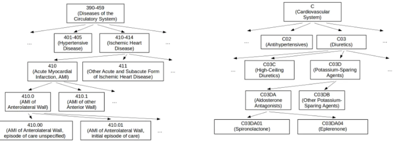
Figure 2-8: Example of hierarchy for ICD-9 diagnosis codes (left) and ATC medication codes (right).

Anatomical Therapeutic Chemical (ATC) Classification System [7]. Billing data are also termed “administrative data.”

ICD-9 Codes

ICD-9 codes [6] were developed by the World Health Organization to standardize disease classification. This enables epidemiological studies of diseases despite the use of different languages or terminology by different physicians or institutions. For ex-ample, the code 250 is standardized to represent diabetes mellitus, the more common form of diabetes.

In our dataset, there are two types of ICD-9 codes, diagnoses and procedures. Diagnosis codes follow the XXX.XX format: three digit codes with two digits after a decimal point. There are also two sets of supplementary codes. The first set starts with “V”: VXX.XX and are used for people who are not currently sick, such as for organ donation and vaccinations, and people who require long-term treatment, such as dialysis. The second set starts with “E”: EXXX.X and identifies the cause of external injuries or poisoning, such as type of motor vehicle accident. ICD-9 procedure codes follow the XX.XX format and are used to indicate the type of operation or procedure that the patient received.

(45)

illustrated in Figure 2-8. For example, 410 represents acute myocardial infarction, or heart attack. In this case (but not for all codes), the fourth digit indicates the specific part of the heart that was damaged, and the fifth digit indicates if this was the first time that the patient was seen for this episode of heart attack.

Going one level up, the digits before the decimal point can be grouped into cat-egories. For example, ICD-9 codes that fall between 390 and 459 are all types of circulatory system diseases. Codes that fall between 410 and 414 are ischemic heart diseases.

Frequently, not all of the digits are used. This is particularly true of digits after the decimal point. This can be due to insufficient information at the time of coding, such as unknown part of the heart that was implicated in a heart attack, or human error.

ATC Codes

ATC codes [7] were also developed by the World Health Organization, and classify drugs according to the organ system that they act on, the class of medication that they fall under, and their chemical properties.

Like the ICD-9, ATC codes are also hierarchical. The ATC hierarchy contains five levels (Figure 2-8). The first level contains a single letter and describes the organ system that the drug acts on. Examples include alimentary tract and metabolism (A), cardiovascular system (C), nervous system (N), and respiratory system (R). The second level contains two digits and indicates the general class of drug. Examples include diuretics (C03, removes water from the body and is used in conditions such as heart failure), and beta blockers (C07, slows down heart rate). The third level contains one letter and is a more specific class than the second. For example, diuretics can be divided into low ceiling (C03A) and high ceiling (C03B), which refer to whether the drug effects can be increased with higher dosage. The forth level consists of one letter and indicates a more specific type of drug. For example, high-ceiling diuretics can be divided into plain sulfonamides (C03CA), aryloxyacetic acid derivatives (C03CC), etc. Finally, the fifth level contains two digits and indicates the specific drug, such as

(46)

furosemide (C03CA01) and bumetanide (C03CA02).

Unlike the ICD-9 codes, the ATC codes are almost always complete, with no missing trailing letters or digits. This is because drug prescriptions have to be precise with respect to the drug name. In rare instances, the ATC codes are incomplete in our dataset. This occurs when the drug used has not been assigned a specific ATC code, and therefore the mapping stops at a higher level.

(47)

Chapter 3 Risk Stratification Using ECG:

Morphological Variability in

Beat-space

3.1 Introduction

Risk stratification after acute coronary syndrome (ACS) involves integrating a di-verse array of clinical information. Risk scores such as the Global Registry of Acute Coronary Events (GRACE) [42] and Thrombolysis In Myocardial Infarction (TIMI) [9] scores aid in this process by incorporating clinical information such as cardiac risk factors and biomarker data. Unfortunately, existing metrics like these only identify a subset of high-risk patients. For example, the top two deciles of the GRACE score and a high TIMI Risk Score (≥ 5) captured 67% and 40% of the deaths, respectively. That a significant number of deaths will occur in populations that are not tradition-ally considered to be high risk highlights a need for tools to discriminate risk further [40]. In this regard, the use of computational biomarkers may provide additional information that could improve our ability to identify high risk patient subgroups [94]. Indeed, several studies showed that ECG-derived computational metrics signif-icantly improve the ability to risk stratify in subgroups with relatively preserved left

(48)

ventricular ejection fraction (EF) [12, 15, 14, 94].

An overview of these risk measures can be found in Section 2.1.4. Briefly, ECG-based metrics can be broadly divided into ones that analyze heart rate changes, and ones that analyze changes in morphology. Examples of heart rate-based metrics in-clude Heart Rate Variability (HRV) [70], Deceleration Capacity (DC) [15], Heart Rate Turbulence (HRT) [84], and Severe Autonomic Failure (SAF) [14]. Morphology based metrics include T Wave Alternans (TWA) [80], which is designed to measure specific alternating changes in cardiac repolarization and Morphologic Variability (MV) [93], which is designed to quantify the beat-to-beat morphologic variability in ECG signals. A key parameter in MV is the diagnostic frequency band of 0.30-0.55Hz. Higher variability in this frequency band is associated with adverse outcomes such as death [93]. In this study, we evaluate the hypothesis that measuring frequency in terms of cardiac cycles (“beat-frequency”) will result in a more accurate risk metric. We term this new metric MV in Beat-space (MVB), and compare MVB with clinical and other ECG risk metrics.

3.2 Methods

3.2.1 Dataset

We used two datasets of ECG recordings in this work, a derivation [25] and a val-idation cohort [67], from two clinical trials of patients with non-ST-elevation ACS (NSTEACS). Patient characteristics of our cohorts are shown in Table 3.1. The derivation cohort consisted of 765 patients, with 14 cardiovascular deaths (CVD) (1.8%) within the median followup period of 90 days. We used the derivation cohort to derive parameters for a new morphologic variability risk metric, MVB, described below). This is the same population that the original Morphologic Variability metric was derived from [93].

We then tested the ability of each ECG-based metric to identify high risk patients on the validation cohort. In order to compare our proposed metric with established

(49)

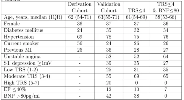
Table 3.1: Patient characteristics for validation cohort and lower risk subpopulations. All characteristics except age and BMI are reported as %. BMI = Body Mass Index; IQR = Interquartile Range; MI = Myocardial Infarction; TRS = TIMI Risk Score; EF = ejection fraction; BNP = B-type natriuretic peptide. -: data not available for the cohort.

Derivation Validation TRS≤4

Cohort Cohort TRS≤4 & BNP≤80

Age, years, median (IQR) 62 (54-71) 63(55-71) 61(54-69) 58(53-66)

Female 36 37 37 36 Diabetes mellitus 24 35 32 34 Hypertension 69 78 75 76 Current smoker 56 24 26 26 Previous MI 25 36 28 27 Unstable angina - 52 52 64 ST depression ≥1mV - 39 35 27 Low TRS (1-2) - 25 31 35 Moderate TRS (3-4) - 55 69 65 High TRS (5-7) - 20 0 0 EF ≤40% - 12 10 7 BNP >80pg/ml - 42 38 0

clinical measures, we only included patients who had measured values for both the left ventricular ejection fraction (EF) and B-type natriuretic peptide (BNP). This population included 1082 patients, with 45 CVD within the median followup period of one year (4.5%).

In addition, we evaluated the performance of these metrics on several subgroups of patients that are considered “low-risk” based on the TIMI Risk Score (TRS), EF, and BNP. These low risk critera are listed in the first column of Table 3.2. We did not use the GRACE risk score because we did not have all the variables required to compute it. The number of patients and CVD in these populations are presented in Table 3.2, sorted by decreasing one year CVD rates. Patient characteristics of representative low-risk subgroups (TRS≤4 and the combination of TRS≤4 and BNP≤80) are shown in Table 3.1.

(50)

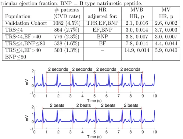
Table 3.2: Number of patients in validation cohort and low risk subgroups, and hazard ratio (HR) of risk metrics Morphologic Variability (MV) and MV in Beat-space (MVB). CVD = cardiovascular death; TRS = TIMI Risk Score; EF = left ventricular ejection fraction; BNP = B-type natriuretic peptide.

# patients HR MVB MV

Population (CVD rate) adjusted for: HR, p HR, p

Validation Cohort 1082 (4.5%) TRS,EF,BNP 2.1, 0.016 2.6, 0.002

TRS≤4 864 (2.7%) EF,BNP 3.0, 0.014 3.7, 0.003

TRS≤4,EF>40 776 (2.3%) BNP 3.8, 0.007 3.0, 0.007

TRS≤4,BNP≤80 538 (1.6%) EF 7.8, 0.014 4.4, 0.044

TRS≤4,EF>40 503 (1.3%) – 14.9, 0.014 5.9, 0.040

BNP≤80

Figure 3-1: Because of instantaneous heart rate changes, cardiac events are periodic only with respect to heartbeats but not with respect to time.

3.2.2 Morphologic Variability in Beat-space (MVB)

Overview

MV measures beat-to-beat variability in ECG morphology in the diagnostic frequency of 0.30 to 0.55Hz. Taking the inverse of these two frequency values give the temporal periods 3.3s and 1.8s respectively, implying that high variability in beat-to-beat ECG morphology every two to three seconds is associated with death. However, because of beat-to-beat variation in heart rate, cardiac activity is periodic with respect to heart beats instead of with respect to time. For example, as illustrated in Figure 3-1, events observed at two-second intervals may correspond to different parts of the ECG waveform. However, by definition, events observed at two-beat intervals correspond

(51)

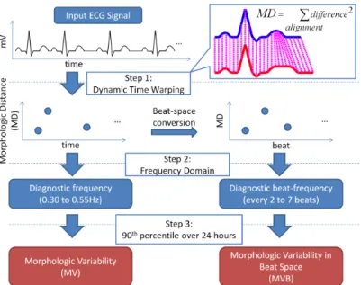
Figure 3-2: Overview of Morphologic Variability (MV) and MV in Beat-space (MVB) computation.

to the same part of the ECG waveform.

Accordingly, we speculated that it might be useful to analyze frequency relative to heartbeats rather than relative to time. This changed the analysis space from time to beats, and consequently changed the frequency domain (units of Hz) to a “beat-frequency” domain (units of cycles/beats).

This concept was first reported as beatquency [57], where it was applied to the heart rate time series to classify sleep stages. The authors found through visual inspection that the beat-frequency spectra were highly consistent in the same subject across different nights, and across different subjects. For ease of interpretation, we report the beat-frequency bands as their inverse, i.e., “every x beats.”

Computation of MVB

We calculated MVB using the first 24 hours of ECG for each patient. Many steps are similar to the MV computation [95]. The important steps are briefly described here, and contrasted with MV in Figure 3-2. We first preprocessed the ECG using the Signal Quality Index [54], to help ensure that only normal beats are studied. Next, we removed baseline wander by subtracting the median filtered signal [31]. Then,

Applying domain knowledge to clinical predictive models

Applying Domain Knowledge to Clinical Predictive

Models

by

Yun Liu

B.S., Johns Hopkins University (2010)

Submitted to the Department of Health Sciences and Technology

in partial fulfillment of the requirements for the degree of

Doctor of Philosophy in Medical Engineering

at the

MASSACHUSETTS INSTITUTE OF TECHNOLOGY

June 2016

c

○

Massachusetts Institute of Technology 2016. All rights reserved.

Author . . . .

Department of Health Sciences and Technology

May 16, 2016

Certified by. . . .

Collin M. Stultz, MD, PhD

Professor

Thesis Supervisor

Certified by. . . .

John V. Guttag, PhD

Dugald C. Jackson Professor

Thesis Supervisor

Accepted by . . . .

Emery N. Brown, MD, PhD

Director, Harvard-MIT Program in Health Sciences and

Technology/Professor of Computational Neuroscience and Health

Sciences and Technology

Applying Domain Knowledge to Clinical Predictive Models

by

Yun Liu

Abstract

Acknowledgments

Contents

List of Figures

List of Tables

Chapter 1

Introduction

1.1 Applying Medical Knowledge to Aid Feature

En-gineering

1.1.1 Motivation

1.1.2 Contributions

1.2 Transferring Medical Knowledge From Text

1.2.1 Motivation

1.2.2 Contributions

1.3 Organization of Thesis

Chapter 2

Background

2.1 Risk Stratification using Electrocardiograms (ECG)

2.1.1 The Heart and ECG

2.1.2 Acute Coronary Syndrome (ACS)

2.1.3 Clinical Risk Metrics

2.1.4 Long-term ECG Risk Metrics

2.1.5 Evaluation and Comparison of Risk Metrics

2.2 Risk Stratification using Health Insurance Records

2.2.1 Transfer Learning

2.2.2 Distributed Representation of Words

2.2.3 Word2vec

2.2.4 Word Vector Properties

2.2.5 Health Insurance Records

Chapter 3

Risk Stratification Using ECG:

Morphological Variability in

Beat-space

3.1 Introduction

3.2 Methods

3.2.1 Dataset

3.2.2 Morphologic Variability in Beat-space (MVB)