Automated modeling of nonlinear dynamical subsystems for stable system simulation

Automated Modeling of Nonlinear Dynamical

Subsystems for Stable System Simulation

by

Yu-Chung Hsiao

Submitted to the Department of Electrical Engineering and Computer

Science

in partial fulfillment of the requirements for the degree of

Doctor of Philosophy

at the

MASSACHUSETTS INSTITUTE OF TECHNOLOGY

I

June

2015

0

Massachusetts Institute of Technology 2015. All rights reserved.

I1+bn ISignature

redacted

Department of Electrical

A7

Certified by.

Luca Daniel

Professor of Electrical Engineering and Computer Science

Thesis Supervisor

Engineering and Computer Science

May 20, 2015

Accepted by...

Signature redacted

65)

Leslie A. Kolodziejski

Chair, Department Committee on Graduate Theses

Signature redacted

Automated Modeling of Nonlinear Dynamical Subsystems

for Stable System Simulation

by

Yu-Chung Hsiao

Submitted to the Department of Electrical Engineering and Computer Science on May 20, 2015, in partial fulfillment of the

requirements for the degree of Doctor of Philosophy

Abstract

Automated modeling techniques allow fast prototyping from measurement or sim-ulation data and can facilitate many important application scenarios, for instance, shortening the time frame from subsystem design to system integration, calibrating models with higher-order effects, and providing protected models without revealing the intellectual properties of actual designs.

Many existing techniques can generate nonlinear dynamical models that are stable when simulated alone. However, such generated models oftentimes result in unstable simulation when interconnected within a physical network. This is because energy-related system properties are not properly enforced, and the generated models er-roneously produce numerical energy, which in turn causes instability of the entire physical network. Therefore, when modeling a system that is unable to generate energy, it is essential to enforce passivity in order to ensure stable system simulation. This thesis presents an algorithm that can automatically generate nonlinear pas-sive dynamical models via convex optimization. Convex constraints are proposed to guarantee model passivity and incremental stability. The generated nonlinear mod-els are suited to be interconnected within physical networks in order to enable the hierarchical modeling strategy.

Practical examples include circuit networks and arterial networks. It is demon-strated that our generated models, when interconnected within a system, can be simulated in a numerically stable way. The system dynamics of the interconnected models can be faithfully reproduced for a range of operations and show an excellent agreement with a number of system metrics. In addition, it is also shown via these two applications that the proposed modeling technique is applicable to multiple physical domains.

Thesis Supervisor: Luca Daniel

Title: Professor of Electrical Engineering and Computer Science

d,-Acknowledgments

First and foremost I would like to express my gratitude to my advisor, Prof. Luca Daniel, for his instruction and guidance for the past several years. His impressive ability to connect concepts has successfully fostered a multidisciplinary research en-vironment, giving me enormous opportunities to learn and work with people from various backgrounds. This work could not have been possible without his support.

I would also like to thank my committee members, Prof. Alexandre Megretski

and Prof. Pablo A. Parrilo for their valuable suggestions on this work. I would like to give special thanks to Alex for his being an extremely patient and insightful guide on my journey through system theory and identification. His tremendous knowledge has greatly influenced my mathematical thinking and communication.

I would like to acknowledge two research groups outside MIT that greatly

con-tributed to my study in cardiovascular systems: Prof. Yuri Vassilevski's group at Institute of Applied Mathematics, Russian Academy of Sciences, and Prof. Hao-Ming Hsiao's Advanced Medical Device Laboratory at National Taiwan University. My appreciation also extends to their members who collaborated closely during my visit: Tatiana Dobroserdova, Timur Tscherbul, and Kuang-Huei Lee.

I would like to thank my colleagues in Computational Prototyping Group, whom

I learned, shared, and spent a great time with. I would like to thank Bradley N. Bond for introducing me to the exciting field of system identification, Amit Hochman for being such an encouraging mentor, Tarek El-Moselhy for sharing many words of wisdom, Zohaib Mahmood for being a nice comrade marching together toward our degrees, Zheng Zhang for many constructive research suggestions, Tsui-Wei (Lily) Weng for always reminding me of the beauty of our hometown, Taiwan, Lei Zhang and Bo Kim for organizing great social events, Jose E. Cruz Serralles and Richard Zhang for many delightful conversations and suggestions on presentations, and also Niloofar Farnoush and Omar Mysore for being excellent officemates.

I wish to express my gratitude to several individuals for their mentoring and

Wasser-man, whom I worked with as a teaching assistant during my first year study, for his generosity, patience, and encouragement. I want to thank Prof. Terry P. Orlando for his wisdom that guided me through different stages of my PhD study. I want to express my deep appreciation to Ching-Kuang Clive Tzuang, Professor Emeritus at National Taiwan University, for his long-term mentoring since college. I would like to thank Dr. Shang-Te Yang for inspirational conversations across various topics.

I would like to especially thank Dr. Yuh-Chwen G. Lee for her long-term support,

listening, and encouragement during the rough spots of this challenging journey. Last but not the least, I would like to thank my family for their endless support, understanding, and love.

Contents

1 Introduction

1.1 Existing Techniques for Passive Model Generation 1.2 Proposed Method and Related Works . . . .

1.3 Scope of Applications . . . .

1.4 Outline and Contributions . . . .

2 Background

2.1 System theory . . . . 2.1.1 Dissipativity and Passivity . . . . 2.1.2 Incremental Stability . . . . 2.2 Sum-of-Squares Optimization . . . .

2.3 Additional Theorems . . . .

3 System Identification for Passive Nonlinear

3.1 Model Structure. . . . .. . . . .

3.2 Convex Constraints . . . .

3.2.1 Bijectiveness Guarantee . . . .

3.2.2 Passivity Guarantee . . . .

3.2.3 Incremental Stability Guarantee . . .

3.3 Objective Functions and Optimization . . .

Dynamical Systems

4 Analysis of Convex Constraints

4.1 Passivity Guarantee . . . . 13 15 16 17 17 21 21 21 23 25 26 29 29 30 30 30 31 32 35 35

4.1.1 For LTI Systems . . . .

4.1.2 For First-Order Single-Port LTI Systems . 4.1.3 _{For Nonlinear Systems with Polynomials e,} 4.2 Incremental Stability Guarantee . . . .

4.2.1 For LTI systems . . . . 4.2.2 For Nonlinear Systems with Polynomials e,

4.3 Proofs . . . . 4.3.1 Proof of Theorem 4.1 . . . . 4.3.2 Proof of Corollary 4.2 . . . . 4.3.3 Proof of Theorem 4.3 . . . . 5 Implementation 5.1 Basis Functions . . . . 5.2 Derivative Estimation. . . . . 5.3 Data Normalization . . . . 5.4 Optimization Tools . . . . 5.5 Simulation Environment . . . .

6 Model Training Practice 6.1 Data Preparation . . . . . 6.1.1 Intended Usage of t 6.1.2 Training Data . . . 6.1.3 Validation Data . . 6.1.4 Test Data . . . . . 6.2 Error Metrics . . . . 6.3 Model Complexity . . . . 6.3.1 Polynomial Degrees 6.3.2 Stiffness . . . . 6.4 Modeling Procedure . . . he Model h

f,

f,

7 Case Studies: Circuit Networks 7.1 Diode RC Line ...

7.1.1 Training . . . .

7.1.2 Validation . . . .

7.1.3 Test within a System . . . .

7.2 Properties of the Algorithm . . . .

7.2.1 Effects of Passivity Guarantee . . . .

7.2.2 Effects of Incremental Stability and Regularization

7.2.3 Effects of Weight rK and Regularization . . . . 7.2.4 Modeling from Noisy Data . . . .

7.3 Class E Power Amplifier . . . .

8 Case Studies: Arterial Networks

8.1 Scenario . . . .

8.2 Geometries and Parameters . . . . 8.3 Assumptions for Fluid Dynamics Simulation . 8.4 Modeling of Aortic Bifurcation . . . .

8.5 Modeling for Iliac Bifurcation . . . .

8.6 Modeling via Interconnecting Local Models 9 Conclusion

9.1 Extensions of Techniques . . . .

9.1.1 Repeated Experiments and Noisy Data

9.1.2 Convex Constraint Related Topics . . .

9.1.3 Model Quality Improvement . . . .

9.1.4 Concepts from Linear Systems . . . . .

9.1.5 Dissipativity in Discrete Time . . . . .

9.2 Further Development of Applications . . . . .

61 . . . . 61 . . . . 62 . . . . 62 . . . . 63 . . . . 66 . . . . 67 . . . . 68 . . . . 68 . . . . 75 . . . . 78 81 . . . . 8 1 . . . . 8 2 . . . . 8 4 . . . . 8 6 . . . . 9 1 . . . . 9 5 101 101 101 102 103 103 104 105

List of Notations

No set of natural numbers including 0

R+ nonnegative real number

[a; b] vertical concatenation of vector a and b

X' transpose of x

time derivative of x

R[x] set of polynomials in x with coefficients in R

[x]d a vector of monomials up to degree d

X >- Y positive definiteness of X - Y

X >_ Y positive semidefiniteness of X - Y

X > Y elementwise xi ;> yij

|XHIQ weighted 2-norm of vector x as IX'QX,

Q

||X

matrix X as Vtr(X'QX),

Q

tr(X) trace of matrix X

Xt _{Moore-Penrose pseudoinverse of matrix X} diag(d) a diagonal matrix with diagonals as entries in d

In an n-by-n identity matrix

Omxn an m-by-n zero matrix

On an n-by-n zero matrix

1 a vector of all ones

ker(X) kernel space of X deg(a) degree of polynomial a

Chapter 1

Introduction

Modeling dynamical systems is the foundation for solving complex engineering prob-lems. Many mature and well-established physics-based models are "handcrafted" through years of trials and errors using domain knowledge. On the other hand, auto-mated techniques have been proposed for fast prototyping and black-box modeling. These capabilities can facilitate many application scenarios, such as shortening the time frame from the design of individual components to their integration into a sys-tem, calibrating models with higher-order effects, and providing protected models without revealing the intellectual properties of actual designs.

The black-box approaches have achieved wide success in generating standalone models [5, 6, 20, 35, 38, 48, 58, 60, 70]. However, when models are interconnected in a physical network, such as electrical circuits, the law of energy conservation must be considered in order to avoid instability artifacts. Such a concept of energy conser-vation is centered on the notion of passivity, i.e., the inability of generating energy. Energy conservation ensures that a system that is formed by interconnecting passive

systems is also passive. In the modeling context, the counterpart statement for

in-terconnecting passive models has also been studied in a similar manner [75]. When passive systems fail to be represented as passive models, numerical energy may be generated. This excess artificial energy oftentimes causes numerical instability of the entire interconnected systems and may even halt the transient simulation due to convergence issues.

Passive systems cover a wide range of practical systems. Any systems that are lossless or energy-consuming (when all supplied power is considered, particularly in-cluding the power from sources) are passive in the sense of energy consumption. In electrical circuits, for instance, almost all circuit networks are passive when sources are excluded. This set includes linear RLC components, nonlinear transistors and diodes, and their combinations, such as power amplifiers or RF mixers. It is impor-tant to note that the traditional classification of active and passive circuits is different from the passivity discussed here. Many circuit networks are traditionally labeled as

active because they can provide incremental or small-signal gain from designated

in-puts to outin-puts. However, when the supplied power from all ports is considered, the vast majority of such so-called active circuits are in fact passive in the sense of energy

consumption. Therefore, such active circuit networks also belong to the set of passive

systems.

This thesis concerns the problem of generating nonlinear passive dynamical models from measurement or simulation data. Several challenges contribute to the difficulty of such a task. First, many existing passive modeling techniques are based on match-ing the poles and zeros of transfer functions to frequency-domain data [15, 41, 62]. However, for nonlinear systems, the concept of frequency is not uniquely defined [11, 14]. Second, while model fitting is preferably performed in the time domain for non-linear systems, their passivity condition [28, 73] is generally non-convex and leads to challenging optimization problems. Although convex relaxation techniques [41, 62] have been proposed to "convexify" the passivity condition for linear modeling, the convex relaxation techniques for nonlinear modeling are relatively scarce, if there is any.

This thesis presents an algorithm that can automatically generate nonlinear pas-sive dynamical models via convex optimization. Convex constraints are proposed to guarantee model passivity and incremental stability. The generated passive models are suited to be interconnected within physical networks for enabling the hierarchical modeling strategy. Two sets of practical examples are demonstrated: circuit networks and arterial networks. It can be seen via these two applications that the proposed

modeling technique is applicable to multiple physical domains.

1.1

Existing Techniques for Passive Model

Gener-ation

Various methods have been proposed for generating linear passive models based on the Positive Real Lemma or the Kalman-Yakubovich-Popov (KYP) Lemma [2], for example, [15, 22, 24, 42, 63]. However, the techniques for automatically generating

nonlinear passive models are relative scarce [37, 79].

Automated passive modeling methods can be categorized into three major types based on the timing when passivity is enforced. The model passivity can be enforced

before, during, or after model parameters are identified.

Guaranteeing Passivity by Construction

Model passivity is guaranteed by restricting model structures such that the model passivity is irrespective of the choice of model parameters. Examples include synthesis of linear models using passive R, L, C, G components [17, 32, 77] and specialized dynamic neural networks for nonlinear systems [37, 79].

Enforcing Passivity Simultaneously during Model Search

Model passivity is enforced simultaneously during model parameters are identified. This is typically done through formulating an optimization scheme such that the optimal model parameters are sought within a constrained set described by a passivity condition. Several existing methods for linear modeling belong to this category, for instance, [15, 41, 63].

Enforcing Passivity by Post-Processing Generated Models

Models are first generated with limited or even without any passivity consideration. Then the model parameters are perturbed or post-processed in order to satisfy certain

passivity criteria. Examples include [23, 25, 42, 72] for the linear case.

To the best of our knowledge, the existing techniques for generating nonlinear passive models are currently restricted to the first type. Prior to this work, there seem no reported results for stable system simulations that incorporate interconnected generated nonlinear models.

1.2

Proposed Method and Related Works

The proposed algorithm is formulated as a sum-of-squares optimization program and guarantees the model passivity using a convex passivity constraint. Such a passivity constraint is a convex relaxation of the dissipation inequality in [73]. The modeling strategy of the proposed method is to search for model parameters within a passivity constraint, and, therefore, belongs to the second type in the classification above. To enhance the model robustness, two additional mechanisms are proposed: incremental stability and the f, regularization. Incremental stability is a system property that requires that, when excited by the same input, any two state trajectories starting from different initial conditions converge to each other over time. In other words, an incrementally stable model is more robust against a perturbation on initial conditions. To guarantee incremental stability, an additional convex constraint is proposed as a convex relaxation of the incremental Lyapunov theory [3, 80] that implies incremental stability. The f, regularization is used to empirically reduce the overfitting problem and perform basis function selections [65].

The approach of this work is closely related to the techniques that identify incre-mentally stable systems [8, 45, 66, 67]. All these four works proposed algorithms based on the sum-of-squares optimization method and involved various incremental stability guarantees and simulation error bounds. No passivity guarantee has been studied in these works. In addition, most of such developments were focused on discrete-time systems, with the exception of [67], half of which is dedicated to continuous-time systems. This thesis, on the other hand, focuses on continuous-time systems and the passivity guarantee that ensures stable simulation of interconnected models.

1.3

Scope of Applications

The scope of this work can be extended to a wide range of applications that are compatible with bond graphs [51], in which the instantaneous power delivered by a bi-directional link is defined as the product of the across and the through variables associated with the link. We list a few examples in Table 1.1. Detailed treatments and surveys can be found in [9, 16, 34, 47].

Table 1.1: Examples of physical networks

Domain Across variable Through variable

Electrical Voltage Current

Magnetic Magnetomotive force Magnetic flux

Mechanical, translation Linear velocity Force

Mechanical, rotation Angular velocity Torque

Hydraulic Pressure Flow

Thermal Temperature Heat flow

1.4

Outline and Contributions

This section outlines the organization of this thesis and summarizes the contributions.

" Chapter 2 gives a brief summary of background that is relevant for the

forth-coming discussions. Topics include the system theory and the sum-of-squares optimization. Among the system theory, passivity and incremental stability are presented. Some prior knowledge is assumed. For example, the basic cir-cuit analysis, the state-space model, and the basics of convex optimization are, therefore, not covered here.

" Chapter 3 develops a convex optimization program that can identify a

nonlin-ear passive dynamical model given a set of training data. A form of nonlinnonlin-ear state-space model is considered throughout this thesis. The convex optimization program minimizes the state-equation errors and the output-equation errors, as a heuristic to search for the best suited model parameters against the training

data. To ensure that the generated models are passive, the optimization pro-gram consists of a convex constraint that serves as the sufficient condition to model passivity. A formal proof is provided to establish such sufficiency to the original passivity condition.

To regularize the behaviors of the generated models, the optimization program is further equipped with two mechanisms: incremental stability and the fi reg-ularization. Similar to the passivity condition, a convex sufficient condition is proposed to ensure that the generated models are incrementally stable. The regularization is used to reduce the overfitting problem. The f, version of the regularization additionally reduces the number of basis functions in the gener-ated models. The resulting convex optimization problem can be formulgener-ated as a sum-of-squares optimization program.

" Chapter 4 presents a number of analyses of the convex passivity and

incremen-tal stability constraints developed in Chapter 3. The restrictiveness due to the sufficiency of the passivity condition is studied using the general LTI case, the first-order single-port LTI case, and the polynomial case. All these three cases show that the output equation in the model structure must algebraically depend on the input signals. Specifically, the analysis using the first-order single-port LTI system visualizes the feasible regions and shows that the convex passivity constraint excludes some low-loss and lossless systems. For the convex incre-mental stability constraint, it is shown that a certain restriction is imposed on the model structure when the models are represented by polynomial functions.

" Chapter 5 provides the implementation details.

" Chapter 6 outlines the model training practice. The modeling procedures include three phases: the training phase generates models, the validation phase determines the training and modeling parameters, and the test phase measures the performance of the generated model when interconnected within a physical network. A few practical considerations are also discussed in this chapter.

" Chapter 7 presents the first set of examples: the application in circuit

net-works. Examples include a diode RC line and a Class E power amplifier. In both cases, stable simulation is performed with good accuracy when the gen-erated models are interconnected within a physical network. Several numerical examples are provided to demonstrate the usefulness of the system properties, the effect of the f, regularization, and the performance of generating models from noisy data.

" Chapter 8 presents the second set of examples: the application in arterial net-works. In particular, the segments from the abdominal aorta to the iliac arteries are considered. The modeling of such arteries is treated in a hierarchical man-ner: generate the local bifurcation models first, and then form a global model

by interconnecting the generated local models. Stable and accurate simulation

is demonstrated for both the local and the global models.

Chapter 2

Background

We briefly review some basic notions in the system theory and the sum-of-squares (SOS) optimization.

2.1

System theory

2.1.1

Dissipativity and Passivity

The earliest development of passivity in systems and circuit networks can be traced back at least to 1950s. Most of the discussions during that period were focused on linear network theory [54, 68, 74, 78] in the form of

v(t)i(t) dt > 0, (2.1)

where v(t) and i(t) are vectors of voltages and currents at the ports of a circuit net-work. The prime notation (') denotes the transpose of the vector. Willems general-ized this concept to dissipativity and explicitly involved system states of a state-space model in an inequality similar to (2.1).

Definition 2.1 (Dissipativity[73]). A dynamical system E

(t) = f(X(t), u(t)) (2.2)

y(t) = h(x(t), u(t)) (2.3)

for t > 0 with inputs u c U, states x E X, and outputs y E Y is called dissipative with respect to a supply rate o-(u, y) if there exists a nonnegative storage function

V, : X '-+ R+ such that the dissipation inequality

V(x(t)) - V(x(O)) <

]

is satisfied for all T > 0 and for all u E U, x E X, y E Y. In addition, if V is

continuously differentiable, then (2.4) is equivalent to

Vs ((t)) a-(u(t), y(t)) (2.5)

for all t> 0 and for all u EU, xE X, y E Y.

Dissipativity is a mathematical abstraction of energy conservation. The dissipa-tivity inequality states that, from (2.4), the increase of internal energy is bounded

by the external supplied energy, or from (2.5), the growth rate of internal energy is

bounded by the external supplied power. The dissipation inequality in (2.4) or (2.5) were derived in multiple ways in literature. Willems' definition in [73] postulates that dissipativity holds whenever a storage function exists. Some others, for instance, Hill and Moylan in [27, 28], begins with the non-negative dissipation

oj-(u(t), y(t)) dt 0, (2.6)

for all T > 0, u E U, y E Y, and then prove the existence of the available storage

function, which is a lower bound of V in (2.4). A range of definitions, treatments, and their relationships can be found in Chapter 4 of [10].

X, and outputs y E Y in the form of (2.2) and (2.3) is called passive if E is dissipative

with respect to -(u, y) = u'y. More generally, let -(u, y) = u'y - eu'u - 6y'y. Then

the system E is called input-strict passive if E > 0, output-strict passive if 6 > 0, and input-output strict passive if both E > 0 and 6 > 0. 0

It should be noted that the passivity we discuss here is in the sense of energy consumption. This definition is different from what is commonly used in circuit design.

The dissipation inequality in Definition 2.2 is symmetric about u and y, which reflects the fact that in physical networks, each terminal is bi-directional, i.e., si-multaneously being input and output. For example, in electrical systems, u and y can be referred to as current and voltage, or vice versa, depending on the modeling convenience.

Passivity is important in physical networks because it is a closure property under interconnection: the interconnection of passive systems is also passive. A passive system that fails to be represented as a passive model may violate the closure prop-erty, potentially causing instability of the entire interconnected system as a numerical artifact. The following theorem states that the admissible interconnection of passive systems is passive. By admissible, we mean that the interconnection has negligible physical lengths, incurs zero energy loss, and forms a set of linear algebraic con-straints such that, for circuits, both Kirchhoff's current and voltage laws (KCL and KVL) hold. For other physical networks, the same statement is applied such that the equivalents of the KCL and the KVL hold.

Theorem 2.3 ([75]). Let a dynamical system E with a state space X be formed by

admissibly interconnecting dynamical systems EZ with state spaces Xi for i = 1, ... , k

such that X = X1 x - -- x Xk. Then if El,..., EZ, are passive, E is passive. 0

2.1.2

Incremental Stability

When the robustness of a dynamical system is considered, incremental stability is of particular interest. Incremental stability suggests that any two trajectories of states

tend to each other when the system is excited by the same input. Formally,

Definition 2.4 (Incremental stability [3, 80]). A dynamical system in the form

of (2.2) with u E U and x E X, is incrementally globally asymptotically stable if there exists a metric d and a KL function 3 such that

d (Xl(t), X2(t))

< 0

for all t > 0 and all trajectories Xi, X2 of (2.2) subject to the same input u E U. El

The function 0(r, s) of class 1CL is a continuous function that belongs to class IC in r and strictly decreasing in s with 3(r, s) -+ 0 as s - oc. A class IC function a(r)

is a continuous, strictly increasing function with a(0) = 0. It is called a IC function

when a(r) -+ oc as r - oc [33]. It can be seen from the definition that over time, the

"memory" of initial conditions fades and the "distance" between trajectories shrinks. Since there is no specialty in the time t = 0 for time-invariant systems, every time

stamp t = to can be treated as initial conditions for the trajectories t > to, suggesting that the system is in general more robust against noises and errors on both initial conditions and state trajectories.

A link between the incremental stability and the incremental Lyapunov function

V(X1, X2) has been established.

Theorem 2.5 (Lyapunov approach to incremental stability [3, 80, 81]). A dynamical

system (2.2) with u E U and x E X, is incrementally globally asymptotically stable if there exists a metric d, a continuously differentiable

function

functions a, d, p such that

a (d(xi,X2)) V(X1, x2)

< T

and

d

-V ( i, 2) -pt (d(xi, 2)) , (2.8)

for all t and trajectories x1 and 2 of (2.2) subject to the same input u E U. The

To aid our analysis, we state a version of the positive real lemma for a linear time-invariant (LTI) descriptor system E(E, A, B, C, D)

E = Ax + Bu, x(0) = 0 y = Cx + Du,

(2.9)

where u, y

C

>-0.

Theorem 2.6 (Positive Real Lemma for (2.9)). The LTI descriptor system E(E, A, B, C, D)

in (2.9) is passive if there exists P = P' >- 0 such that

-E'PA - A'PE C - B'PE C'- E'PB D+D' u] (2.10) 0

2.2

Sum-of-Squares Optimization

A sum-of-squares (SOS) program is an optimization problem which minimizes a linear

objective function within a feasible set defined by a set of SOS constraints:

minimize c'O

OER-subject to pj(x; 9) : SOS(x), i = 1, ... , N,

where SOS(x) denotes the set of sum-of-squares of polynomials of variables x E R , and pi(x; 9i) E R[x] of degree 2d are affine in 9. A polynomial p(x) is SOS if there exists qj(x) E R[x] such that

p (X qj?(X),VX. (2.12)

Such a sum-of-squares decomposition is a sufficient condition to guarantee p(x) > 0 for all x.1 In general, determining the nonnegativeness of a polynomial of degree greater than or equal to four is an NP-hard problem [7], whereas searching for qj (x) in (2.12) is a polynomial-time semidefinite programming (SDP) problem. SOS can be related to SDP by

p(x) = [x]'Q[X]d, Q = Q' > 0, (2.13)

where [X]d is a vector of monomials up to degree d. Finding a SOS decomposition in (2.12) is equivalent to searching for a constant symmetric positive-semidefinite ma-trix

Q

polytope of a polynomial p(x) E R[xi, ... , x,] is the convex hull of the exponents of

the monomials in p(x). It has been shown in [55] that if a polynomial p(x) is SOS decomposed as in (2.12), then the Newton polytope of qj and p is related by

.A(qj) C -.M(p), (2.14)

2

where K(-) denotes the Newton polytope of a polynomial. More details can be found in [40, 50, 64].

2.3

Additional Theorems

We will utilize the following result in our later discussion.

Theorem 2.7 ([52]). Let T : R' -+ R' be a continuous function which is strongly

monotone for any x, y such that

(x - y)' (T(x) - T(y)) > EIIx - y1 2, E > 0. (2.15)

Then T(x) =0 has a unique solution. I

'The existence of a sum-of-squares decomposition is also a necessary condition for p(x) > 0 for all x when (i) n = 1, (ii) 2d = 2, and (iii) n = 2,2d = 4. See [7].

If T is strongly monotone, it can be seen that T(x) = T(x) - c for all c E R' is

also strongly monotone and there exists a unique solution for every T(x) = c. One

Chapter 3

System Identification for Passive

Nonlinear Dynamical Systems

In this chapter, we propose a system identification algorithm that generates pas-sive nonlinear dynamical systems via convex optimization. Given a set of training data, the optimization program minimizes the equation errors and searches for model parameters. We propose a sufficient passivity guarantee that serves as a convex con-straint in the optimization program.

3.1

Model Structure

We focus on the following continuous-time state-space model

e(X(t)) = f (X(t), u(t)), x(0) = XO,

dt (3.1)

y(t) = h(x(t), _u(t)),

where u E U E R', x E X E R", and y E Y C R' are inputs, states, and outputs,

respectively, and e(.) is bijective and continuously differentiable for all x with

A

E(x). We further require e,

f,

#2

where 6_{aj E R and a = e,}

_f,

param-eterized by 0 = [Oe; 7; Oh]. We further denote e = eo,

f

their parameter dependency if necessary.

3.2

Convex Constraints

In this section, we propose a set of linearly parameterized constraints that are com-patible with the SOS optimization.

3.2.1

Bijectiveness Guarantee

We require e(.) to be strongly monotone to ensure that e(-) is a bijection. By Theo-rem 2.7 and de(x) = E(x), it can be seen that e(-) is a bijection if

v'E(x)v > EIIVI12 (3.2)

for all x, v E Rn.

3.2.2

Passivity Guarantee

Theorem 3.1. Let E be a dynamical system in the form of (3.1), -(u, y) be a supply rate. If there exists a Q = Q' >- 0 such that the inequality

2a-(u, h(x, u)) + 2x' (e(x) - f(x, u)) - ||xH1

(3S.3)

- 2q' (e(x) + f (x, u)) + ||ll 2 0

is satisfied for all u, x, q, then E is dissipative with respect to -(u, y). El

Proof. Use the inequality 2a'b ; IlaI11 + Ib 1 and let P =

Q

becomes

Then minimize the left-hand side with respect to q, i.e., q = P(e

+

f):

2-(u, h(x, u))+ Ie f| 1 - |Ie + f 112 >0,

which is equivalent to (2.5) by setting V(x) =

Ile(x)H

Corollary 3.2. A dynamical system in the form of (3.1) is passive if there exists a

Q =

Q'

u'h(x, u), i.e.,

2u'h(x, u) + 2x' (e(x) - f (x, u)) - I|xI12

- 2q' (e(x) + f (x, u)) + |II||2 > 0

for all u, x, q.

Proof. The proof follows immediately from Theorem 3.1 and Definition 2.2.

3.2.3

Incremental Stability Guarantee

To improve the robustness of the generated models, inspired by [66], we propose the following constraint as an incremental stability certificate.

Theorem 3.3. Let E be a dynamical system in the form of (3.1) and e > 0. If there

exists a

Q

Q'

2Z' (6e - 6f) - ||A||2 - 2v' (6, + 6f) + ||v||2

Q Q _(3.7)

- 2ew'6e + ||W||2 > 0

is satisfied for all u, x, A, v, w, where

6e = e(x + A) - e(x),

6f= f(x+Au) - f(xu),

then E is incrementally globally asymptotically stable with respect to d(xi, x₂) = El I|e(x1) - e(x2)||Q-1. (3.5) U (3.6) D (3.8) (3.9)

Proof. Similar to the proof for Theorem 3.1, using the inequality 2a'b < a1+ 1_

and minimizing the expression with respect to v and w, i.e., v = P(6e + 6f) and W = P6e, gives

26'P of < - -1El e 11 |2, (310)

where P =

Q-

dt1

dt |le(xi) - e(X2) |2 < - 2Elle(Xi) - e(X2) |21 (3.11)

for all x1 and X2. Since e(-) is invertible, it can be checked that d(xi, x2) = Ile(Xi)

-e(X2)||P is a metric. Choosing p(r) = !Er2 and V(Xi, X2) = |le(Xi) - e(X2)l12 shows

that the system

x = E(x)<f(x,u), (3.12)

is incremental globally asymptotically stable, and so is (3.1).

3.3

Objective Functions and Optimization

Given a set of training data = {'(ti), z(ti), Q(ti), (t ) i = 1, ... , N} and a weight

K > 0, we consider the least squares of equation errors of (3.1)

N N

Jr(,) = I E (zi) * - f(ii, i) 12 + K

>

where we use subscript i to denote the corresponding variable at ti. It is worth noting that even if we are dealing with a continuous-time model, the training information is still sampled at discrete-time points. In addition, minimizing (3.13) provides mini-mized local equation errors from models within the constrained set (3.6), (3.7). The actual output errors I|y(t) -

Q(t)l

min-imized. During the simulation of (3.1), it is possible that u and x deviate away from the training condition due to numerical errors. Therefore, it is important to

desensitize the functions e,

f,

JA() = J(-) + A1|011p. (3.14)

This fp regularization empirically alleviates the overfitting problem and tends to result in more uniform and comparable coefficients of basis functions. We are particularly interested in choosing p = 1 as it additionally introduces sparsity in 6 for basis

function selections [30, 65].

The objective function Ja,A( ) can then be cast into an SDP problem

minimize t,a,b,cER,O subject to t + A1'c t a b a 1 0 0, b 0 r-al 07 0 C + 0 N

a2 >

IIE(

IEQi)ixi

N

b2 _{> j - h(zi,6)|I}2_.

(3.15)

The last two inequalities are second-order cones, which are compatible with SDP through further transformations.

The complete optimization program consists of the objective function with the f regularization in (3.14), the bijectiveness guarantee in (3.2), the passivity guarantee in (3.6), and the incremental stability guarantee in (3.7), given a training data set E,

and parameters t, and A.

minimize 9,Ql,Q2 subject to

Jr,A()

(3.2) for bijectiveness of e(.), (3.6) with

Q

(3.7) with

Q

(3.16)

It is worth noting that c > 0 is automatically fulfilled in (3.15) and the positive

definiteness of Q, and Q2 is implicitly implied by (3.6) when u, x = 0 and by (3.7)

when u, x, A, w = 0, respectively. The f, regularization and the incremental stability

constraint are not required for generating passive models. However, both mechanisms improve the usability of models, as will be shown by examples in Section 7.

Chapter 4

Analysis of Convex Constraints

In this chapter, we analyze some properties of the convex passivity guarantee (3.6) and the convex incremental stability guarantee (3.7).

4.1

Passivity Guarantee

4.1.1

For LTI Systems

We impose the passivity guarantee (3.6) on the LTI descriptor systems in (2.9) and compare the corresponding conditions with the positive real lemma in Theorem 2.6.

A major conclusion is that D + D' needs to be full-rank in the generated models.

Hence, the lossless cases are not included in the feasible set.

Theorem 4.1. Let E(E, A, B, C, D) be an LTI descriptor state-space system with

x(O) = 0 as in (2.9). The passivity constraint in (3.6) is equivalent to

E -A+E'-A'-Q _{C'-B -(E+ A)]}

C - B' D + D' -B' > 0, (4.1)

-(E + A) -B

Q

implies

-E'PA - A'PE - !(E - A -

Q)'P(E

Q)

D + D'_- 0, (4.3)

IBI12 ,P < tr(D + D'), (4.4)

||C - B'(DD)t tr(E - A + E'- A'- Q). (4.5)

Furthermore, if D + D' is not full-rank, i.e., rank(D + D') = m, < m, then there exists an invertible U EE R"'x such that

BU =

L

for some 3, C' E R nx"r . And if u(t) E ker(D + D'), then

u(t)'y(t) = 0. (4.7)

Proof. See Section 4.3.1.

In the theorem, tr(.) and (-)t denote the trace and the Moore-Penrose pseudoin-verse of a matrix, respectively. We define 11 -

||Fp

IIXI1 p = tr(X'PX) = ||xi|2, (4.8)

where X (E R"'x, P E Rxm", and X = [x1, x2, ... , x].

We can draw the following observations for LTI descriptor systems by comparing Theorem 4.1 with the positive realness in Theorem 2.6:

1. The constraint (4.2) implies the positive semidefiniteness of the first principal

is identical to the 2nd principal block matrix.

2. According to the Positive Real Lemma stated in Theorem 2.6, if D + D' is rank-deficient and rank(D + D') = mr, it can be derived that there also exists an invertible U

E

(C' - E'PB)U =

[R

for some R E Rnxmr. This implies that there are common columns in C'U and E'PBU. Theorem 4.1 requires a more restrictive condition (4.6), in which the common columns are identical to zeros.

3. A non-trivial model that satisfies the passivity constraint (3.6) has to be

input-strict passive. This can be concluded from (4.6) or directly from (3.6) by check-ing the highest degree of u. In practice, a full-rank D + D' is preferable. As suggested in (4.7), if D + D' is not full-rank, there exists certain nonzero input signals such that the power consumption of the model is instantaneously zero for all time. Such behaviors are unlikely from a practical system and, therefore, of less interest. The matrix D can be physically interpreted as a resistive network attached between terminals, resulting in resistive energy loss.

4. The conditions (4.4) and (4.5) are extra constraints compared to the positive real lemma (2.10), stating that the "range" of the matrix B and the difference between B' and C are "bounded" by some metric of other parameters.

These additional restrictions come from the convex relaxation (3.6) of the original passivity condition (2.5). To enlarge the feasible set, scaling the state equation by a positive factor, i.e., E(E, A, B, C, D) = E(kE, kA, kB, C, D) with k > 0, provides an extra degree of freedom.

Corollary 4.2. Let E(kE, kA, kB, C, D) be an LTI descriptor state-space system as

in (2.9). The passivity constraint in (3.6) is equivalent to E- A+ E' -A' -

Q

K

Q

for some

Q

Q'

>-

vkB 11,2P < tr(D + D'), 11C - Vk B'I1(D+D')t < tr(E - A + E' - A' -

Q).

Therefore, we intentionally leave the state equation unnormalized in the optimiza-tion program (3.16). The scaling factor k is implicitly determined by the weight of the output equation errors K and the regularization parameter A as formulated in (3.13).

In comparison, for the Positive Real Lemma (2.10), state equation scaling does not affect the feasible region. This can be seen from scaling E, A, and B in (2.10).

-(kE)'P(kA) - (kA)'P(kE)

-L C - (kB)'P(kE)

C/ - (kE)'P(kB) _0.

D+D'

The inequality (4.13) returns to the original one (2.10) when the factor into the free variable P.

(4.13)

4.1.2

For First-Order Single-Port LTI Systems

The feasible region of the passivity constraint (3.6) can be visualized on a two-dimensional plane if we consider a first-order single-port LTI system. Because positive scaling of the input and the output preserves the passivity property, it is sufficient to

[

study the following normalized system

x = -ax + u (4.14)

y = x + du, (4.15)

which we denote as E(1, -a, 1, 1, d). The corresponding transfer function is

1

T(s) = + d. (4.16)

s+a

It can be seen that when a > 0 and d > 0, the system E(1, -a, 1, 1, d) is passive.

The following theorem resolves the feasible region of the passivity constraint (3.6) for the system E(1, -a, 1, 1, d)

Theorem 4.3. Let E be the first-order single-port LTI descriptor system in (4.14)

and (4.15) with a > 0. The passivity constraint in (3.6) is equivalent to

2+2a-q 0 -(1 - a)

0 2d -1 > 0, (4.17)

-1- a) -1 q

for some q > 0. The corresponding feasible region on the d-a plane is bounded by

1 1

d > - and ad > - (4.18)

-8 -8

which is depicted in Figure 4-1. Proof. See Section 4.3.3.

In comparison, the original feasible region due to the positive real lemma is the first quadrant a, d > 0. The passivity constraint (3.6) on the normalized first-order

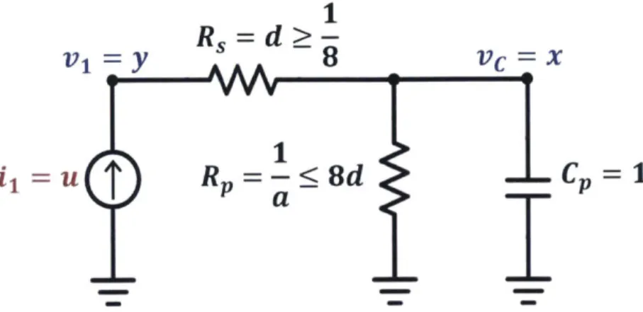
single-port LTI system (4.14) and (4.15) requires additional margins (4.18) from both axes. Therefore, some lossless or low-loss cases are excluded. A circuit analogy for such restrictions is made in Figure 4-2, in which both the series resistor R, and the

2 1.8 1.6 1.4 1.2 T 1 0.8 0.6 0.4 0.2 0 0 0.2 0 4 0.6 0.8 1 d (a) 105 104 103 S102 10 10 10 10- . (/,2 ) 10-1 100 d (b)

Figure 4-1: Feasible region for the convex passivity constraint (3.6) on the normalized scalar LTI system (4.14) and (4.15) in (a) the linear scale and in (b) the log-log scale.

1

RS

=d>-V1=y

1

ii =u

RP =-<

8d

CP = 1

aI

I

Figure 4-2: Circuit analogy of the normalized scalar LTI system in (4.14) and (4.15). The passivity constraint (3.6) requires the series resistor R, to be bounded away from short-circuit and the parallel resistor Rp to be bounded away from open-circuit. The values of R, and Rp determine the loss of the generated system.

parallel resistor R, are restricted to be finite according to (4.18).

4.1.3

For Nonlinear Systems with Polynomials

e,

f,

and h

In this section, we assume e,

f,

f,

Theorem 4.4. Let E be a dynamical system in the form of (3.1) and assume there

exists

Q

Q'

u'h(0, u) > 0, (4.19)

for all u. Polynomial f(x, 0) is either 0 or odd-degree, and

x'f(x, 0) ; 0, (4.20)

deg(h) deg(f2). E

Proof. Let q = -x and (3.6) becomes

u'h(x, u) + 2x'e(x) > 0, (4.21)

for all u, x. If h(x, u) = _{h(x), then (4.21) cannot be satisfied for all u. This shows} that h(x, u) must depend on u. The inequality (4.19) can be derived from (4.21) with

x = 0.

For polynomial

f,

Last, we prove deg(h) > deg(f2) under the assumption f(x, u) = fi(x) + f2(u).

Without loss of generality, assume h(x, u) = H,(x, u)x+h2(u) and deg(h) = deg(h2).

Substituting q = x into (3.6) gives

U'h2(u) - 2x'f2(u) + u'H1(x, u)x - 2x'fi(x) 0, (4.22)

for all u, x. We would like to examine the coefficients for the highest degree of u and determine whether (4.22) can be satisfied. Since deg(h) = deg(h2), deg.(u'Hi(x, u)) <

deg(u'h2(u)). Therefore, the third term is not decisive in determining the

non-negativity for all u. Consider the first two terms. Assume deg(f2) > deg(h). Then

deg(f2(u)) > deg(u'h2(u)). The terms with the highest n-th degree of u can be

collected from u'h₂

(u)

polyno-mials p(x) is linear in x. Since it is not possible to parameterize p(x) such that p(x) is bounded from below, (4.22) is not satisfiable. This concludes that deg(h) > deg(f2).

U

Since the convex passivity constraint (3.6) is a sufficient condition for the original passivity inequality (2.5) with V(x) = jjje(x)j2p, it can be expected that some

afore-mentioned conditions may also be applicable to (2.5). In fact, (4.19) and deg(f2) < deg(h) when f(x, u) = fi(x) + f2(u) and deg(h) = deg(h(0,u)) can be identically

derived. The condition similar to (4.20) is

e'(x)Pf _{(x, 0) < 0,} (4.23)

for all x. The polynomial h(O, u) is odd-degree, or h(x, u) = h(x), the latter of which

requires f to be affine in u as f(x, u) = fi(x) + G(x)u such that

e'(x)PG(x) = h'(x). (4.24)

The conditions in (4.23) and (4.24) together are called the Hill-Moylan condition [71] with respect to VI(x) = 1||e(x)||j. Polynomial f(x, 0) is similarly required to be either odd-degree or 0.

4.2

Incremental Stability Guarantee

4.2.1

For LTI systems

The structural similarity between the passivity constraint (3.6) and the incremental stability constraint (3.7) stimulates the interest in comparing their feasibility condi-tions. In the following, we compare (3.6) and (3.7) on the LTI descriptor systems (2.9).

Theorem 4.5. Let E be an LTI descriptor state-space system (E, A, B, C, D) as

in (2.9) and M = E - A + E' - A' -

Q.

M -(E + A)

-eE

-(E + A)' EE'

Q

On EQ

is satisfied. The positive semidefiniteness of (4.25) implies

-E'PA - A'PE >-

!(E

Q)'P(E

Q)

E + E'- (A + A') >- Q + eE'PE.

(4.25)

(4.26) (4.27)

D

The proof is similar to Theorem 4.1 and, therefore, omitted. By comparing Theo-rem 4.1 and 4.5, it can be seen that (4.2) and (4.26) are identical, and (4.27) is more restrictive than the positive semidefiniteness of the first diagonal block matrix in (4.1)

by an additional term FE'PE. In other words, for LTI systems, the incremental

sta-bility constraint (3.7) imposes a similar yet more restrictive condition on E and A compared to the passivity constraint (3.6). Note that this similarity is limited to the LTI case and does not extend to general nonlinear systems.

4.2.2

For Nonlinear Systems with Polynomials

e,

f,

and h

Similar to the convex passivity constraint, we assume e, f, and h in the model struc-ture (3.1) are polynomials without the constant terms, i.e., e(O) = 0, f(0, 0) = 0, and

h(0, 0) = 0. We would like to examine the degrees of polynomials e,

f,

incremental stability constraint (2.7) and identify the corresponding restrictions on the model structure.

Theorem 4.6. Let E be a dynamical system in the form of (3.1) and assume there

exists

Q

all u, x, A, v, w. Then f (x, u) = fi(x) + f2(u) for some polynomials fi and f2.

Proof. Let w = 0 in (3.7). Rearranging the resulting inequality gives

2(A - v)'6e (x, A) - 2(A + v)'6f (x, A, u) - A'Q A + v'Qv > 0, (4.28)

for all u, x, A, v. We would like to examine the highest degree of u in (4.28) in order identify the restrictions on

f.

form fi(x) + f2(u). Then there exist xO, AO such that f(xo + Ao, u) - f(xo, u) is a

case, the coefficient at ud in

-2(Ao + v)' 6f (xo, Ao, u) (4.29)

is a non-constant linear function of v and, hence, can be made negative by an ap-propriate selection of v = vo such that (4.29) tends to minus infinity as u approaches

infinity, which contradicts (4.28).

4.3

Proofs

4.3.1

Proof of Theorem 4.1

1. Substituting e(x) = Ex, f(x, u) = Ax + Bu, and h(x, u) = Cx + Du into (3.6)

gives, for all x, u, q,

x M C' - B -(E + A)' x

U C-B' D+D' -B' U

q -(E + A) -B

Q

> 0, (4.30)

which implies the positive semidefiniteness of (4.1).

2. The constraints (4.3) follows immediately from the positive semidefiniteness of the second diagonal block matrix.

3. Consider the principal submatrix

D + D'

- B

-B]

Q

(4.31)

Use the Schur complement and the fact

Q