HAL Id: hal-01704395
https://hal.archives-ouvertes.fr/hal-01704395
Submitted on 16 May 2018
HAL is a multi-disciplinary open access
archive for the deposit and dissemination of
sci-entific research documents, whether they are
pub-lished or not. The documents may come from
teaching and research institutions in France or
abroad, or from public or private research centers.
L’archive ouverte pluridisciplinaire HAL, est
destinée au dépôt et à la diffusion de documents
scientifiques de niveau recherche, publiés ou non,
émanant des établissements d’enseignement et de
recherche français ou étrangers, des laboratoires
publics ou privés.
forest landscape
Caroline Greiser, Eric Meineri, Miska Luoto, Johan Ehrlén, Kristoffer
Hylander
To cite this version:
Caroline Greiser, Eric Meineri, Miska Luoto, Johan Ehrlén, Kristoffer Hylander. Monthly
microcli-mate models in a managed boreal forest landscape. Agricultural and Forest Meteorology, Elsevier
Masson, 2018, 250-251, pp.147 - 158. �10.1016/j.agrformet.2017.12.252�. �hal-01704395�
Contents lists available atScienceDirect
Agricultural and Forest Meteorology
journal homepage:www.elsevier.com/locate/agrformet
Monthly microclimate models in a managed boreal forest landscape
Caroline Greiser
a,b,⁎, Eric Meineri
a,c, Miska Luoto
d, Johan Ehrlén
a,b, Kristo
ffer Hylander
a,baDepartment of Ecology, Environment and Plant Sciences, Stockholm University, SE-106 91 Stockholm, Sweden bBolin Centre for Climate Research, Stockholm University, SE-106 91 Stockholm, Sweden
cAix Marseille University, University of Avignon, CNRS, IRD, IMBE Marseille, France
dDepartment of Geosciences and Geography, University of Helsinki, P.O. Box 64 (Gustaf Hällströmin katu 2), 00014, Finland
A R T I C L E I N F O
Keywords: Canopy cover Cold air pooling Climate change Topoclimate Climate variability Forest management
A B S T R A C T
The majority of microclimate studies have been done in topographically complex landscapes to quantify and predict how near-ground temperatures vary as a function of terrain properties. However, in forests understory temperatures can be strongly influenced also by vegetation. We quantified the relative influence of vegetation features and physiography (topography and moisture-related variables) on understory temperatures in managed boreal forests in central Sweden. We used a multivariate regression approach to relate near-ground temperature of 203 loggers over the snow-free seasons in an area of∼16,000 km2to remotely sensed and on-site measured variables of forest structure and physiography. We produced climate grids of monthly minimum and maximum temperatures at 25 m resolution by using only remotely sensed and mapped predictors. The quality and pre-dictions of the models containing only remotely sensed predictors (MAP models) were compared with the models containing also on-site measured predictors (OS models). Our data suggest that during the warm season, where landscape microclimate variability is largest, canopy cover and basal area were the most important microcli-matic drivers for both minimum and maximum temperatures, while physiographic drivers (mainly elevation) dominated maximum temperatures during autumn and early winter. The MAP models were able to reproduce findings from the OS models but tended to underestimate high and overestimate low temperatures. Including important microclimatic drivers, particularly soil moisture, that are yet lacking in a mapped form should im-prove the microclimate maps. Because of the dynamic nature of managed forests, continuous updates of mapped forest structure parameters are needed to accurately predict temperatures. Our results suggest that forest management (e.g. stand size, structure and composition) and conservation may play a key role in amplifying or impeding the effects of climate-forcing factors on near-ground temperature and may locally modify the impact of global warming.
1. Introduction
Forest floor microclimate directly and indirectly influences many biological processes and patterns in forests, such as plant regeneration and growth, species distribution, carbon- and nutrient cycling, soil re-spiration, and soil development (Bonan and Shugart, 1989;Nilsson and Wardle, 2005). In forests, understory microclimates are created by physiographic features, but also by forest structure and composition, creating conditions of higher humidity, decreased wind speed, lower incoming and outgoing radiation (Geiger et al., 2012). Therefore, un-derstanding and modelling forest microclimate is greatly needed to understand spatial and temporal variation in biological processes. Not least in the context of climate change, this knowledge will help to identify efficient strategies to adapt forest management to important
societal goals, such as wood production, carbon sequestration and biodiversity conservation.
The effects of landscape physiography on near-ground tempera-tures, in terms of incoming solar radiation modified by slope and as-pect, pooling of cold heavy air in depressions, adiabatic decrease in temperature towards higher elevations and the moderating influence of soil moisture, air humidity and water bodies have been well studied (Aalto et al., 2017;Dobrowski, 2011;Geiger et al., 2012;Meineri and Hylander, 2016). Vegetation, on the other hand, can have substantial effects on microclimate by canopy shading, evaporative cooling, re-duced wind speed, resulting in rere-duced lateral transfer of humidity and heat, buffering against heat loss overnight and changes in absorbance of shortwave radiation by differences in albedo (Geiger et al., 2012;
Rosenberg, 1974) – referred to as biophysical processes sensu Lenoir
https://doi.org/10.1016/j.agrformet.2017.12.252
Received 22 May 2017; Received in revised form 13 December 2017; Accepted 15 December 2017
⁎Corresponding author.
E-mail addresses:[email protected],[email protected](C. Greiser),[email protected](E. Meineri),miska.luoto@helsinki.fi(M. Luoto),
[email protected](J. Ehrlén),kristoff[email protected](K. Hylander).
Available online 27 December 2017
0168-1923/ © 2018 The Authors. Published by Elsevier B.V. This is an open access article under the CC BY-NC-ND license (http://creativecommons.org/licenses/BY-NC-ND/4.0/).
et al. (2017). In contrast to physiography, vegetation is influenced by
land management, which may have important implications for the microclimate (Frey et al., 2016). Forest management activities, that have the potential to affect the microclimate, include clear-cutting, thinning, green-tree retention, tree planting, choice of tree species as well as the size and distribution of management units (Latimer and Zuckerberg, 2016; Vanwalleghem and Meentemeyer, 2009). Thus, identifying the biophysical processes shaping understory climate (as e.g. inFrey et al., 2016) can enable adaptation to climate change by for example managing the forest in a way that creates favoured micro-climates (De Frenne et al., 2013).
The field of microclimate modelling is currently boosted by the upcoming of cheap climate loggers, the increasing quality and avail-ability of remote sensing products (e.g. high-resolution surface mapping with LiDAR producing digital elevation models or canopy maps, see overview inHe et al., 2015), the growing computational power and the development of new statistical techniques (Keppel et al., 2012;Lenoir et al., 2017). Up to now, the majority of the predictive models have been done in montane landscapes or other types of complex terrain, accounting for local physiography (Ashcroft and Gollan, 2012; Frey et al., 2016;Fridley, 2009;Lookingbill and Urban, 2003;Vanwalleghem and Meentemeyer, 2009). Only a few studies have included also vege-tation features, despite its recognized importance in e.g. buffering temperature extremes (seeTable 1. inLenoir et al., 2017, for a review on microclimate studies including physiographic and biophysical pro-cesses). One reason for the lack of vegetation characteristics in micro-climate models is the lack of high-resolution maps of vegetation structure. Recent provision of e.g. laser scanning measurements of ca-nopy cover and stand density (Larsson et al., 2016;Means et al., 2000) is now opening up for a move from simple measurements along trans-ects (Chen et al., 1996) to spatial predictions over large areas providing high-resolution maps at a 0.5–100 m grain size (Lenoir et al., 2017). However, microclimate modelling is still in its infancy and there is a need for more work in managed forested landscapes, particularly in areas characterized by minor topographic gradients (e.g. as inGeorge et al., 2015). Boreal forests are still underrepresented in microclimate modelling (but seeChen et al., 1996,1993;Chen and Franklin, 1997), which is unfortunate since they form the largest global terrestrial carbon storage (Anderson, 1991) and the world’s second largest biome (Ruckstuhl et al., 2008) with special characteristics (e.g. a dominance of coniferous trees and dwarf shrubs) making extrapolation from other types of vegetation difficult.
Both spatial patterns of microclimate and influences of different climate-forcing factors are likely to vary over different time scales. For instance, forestfloor temperature heterogeneity is larger during the day than at night (Chen and Franklin, 1997) and cold air pooling in topo-graphic depressions can mainly be observed in clear wind-still nights (Dobrowski, 2011). Especially at higher latitudes and in mixed forests
canopy cover, solar angle and their combined effects with topography undergo strong seasonal changes (Lenoir et al., 2013). Temperature extremes during different seasons are limiting for some organisms, when their physiological tolerances are exceeded (Ashcroft et al., 2011;
Meineri et al., 2015;Walther et al., 2009;Zimmermann et al., 2009). Additionally, locations with unusual climates (at the extreme ends of temperature gradients) may play a crucial role as future climate refugia (Ashcroft et al., 2012). While many studies have modelled minimum and maximum temperatures (e.g.Fridley, 2009; Geiger et al., 2012;
Lookingbill and Urban, 2003; Meineri et al., 2015), only few have considered also seasonal changes in climate-forcing factors and their relative influence on near-ground temperatures (e.g. Ashcroft and Gollan, 2013a).
In this paper, we investigate the relative importance of vegetation versus physiography for maximum and minimum temperatures across different snow-free seasons in a lowland boreal forest landscape, in which we expect forest structure and management to play the dominant role in moderating microclimate. Our aims were: (i) to quantify spatial variation in near-ground temperatures in a managed forest landscape, (ii) to examine the relative importance of physiographic and vegetation drivers across seasons and (iii) to predict monthly minimum and maximum temperatures at a 25 m resolution by using only remotely sensed and mapped predictors.
To achieve this, we analysed temperature data from 203 loggers stratified according to physiographic and vegetation gradients across an area of∼16,000 km2. We modelled monthly extreme (minimum and maximum) temperatures in two sets of models. First, we used all available site information, in terms of on-site measured and remotely sensed variables of physiography and forest features, to predict near-ground temperatures. Second, we used only remotely sensed variables available in a mapped form, to produce temperature maps.
2. Methods
2.1. Study area
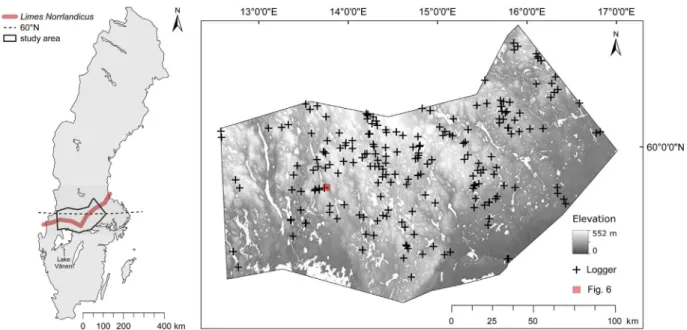
Our study area stretches 190 km across central Sweden (59 to 61° North and 12.5 to 17° East), covering the majority of the quite sharp transition zone "Limes Norrlandicus" (Fig. 1). In this region, the southern boreo-nemoral forest (mixed forest) meets the northern boreal forest (coniferous forest) and many northern or southern forest species have their range limit or change dramatically in abundance in this transition zone (Rydin et al., 1999;Sjörs et. al, 1965). Within this area we focus on forests (16,135 km2 of the study area), which are dominated by spruce and pine with some deciduous elements. The field layer is dominated by ericaceous dwarf-shrubs, mosses and lichens. Almost all boreal forest in Sweden is of secondary nature and has been cleared at least once during the past 200 years (Östlund et al., 1997). Sweden’s
Table 1
Predictors used to model monthly averages of daily minimum (Tmin) and maximum (Tmax) temperatures. Mean and range are for the observation points, not for the entire study area. OS = model containing on-site measured predictors. MAP = model containing only remotely sensed predictors. log = log-transformed. sqrt = square-root-transformed.
Predictor unit abbrev. min mean max Tmin OS Tmin MAP Tmax OS Tmax MAP distance to lake Vänern km distvan 4.68 84.97 173.65 x x x x distance to water km log_distwat 0.03 1.13 5.96 x (log) x (log) x (log) x (log) relative elevation 500 m m log_reel500m 0.54 25.89 125.23 x (log) x (log) – – solar radiation example for December (July) MW sr 0.0001 (0.1210) 0.0001 (0.1487) 0.0003 (0.1623) – – x x elevation m alt 30.58 216.27 477.88 x x x x soil moisturea m soilmoist −2.50 −1.49 0.00 x – x –
distance to forest edgea m distedge 0.00 83.45 250.00 x – x –
proportion of conifersa % conif 0.00 85.58 100.00 x – x –
canopy covera % canopy/ canopy2 0.00 45.96 83.12 x (sqrt) – x –
basal areaa m2/ha basal_area 0.00 12.48 40.00 x – x –
topographic wetness index – twi 4.62 7.20 13.83 – x – x basal area m2/ha BasAre.R 0.00 15.48 43.00 – x – x
Fig. 1. Left: study area in a geographical context. Right: study area with underlying digital elevation model (lakes and rivers in white) and 203 sampling sites equipped with iButton loggers having recorded three-hourly temperature at ground level from June 2015 to August 2016. Sites were selected to represent the panel of physiographic and forest features available within the studied landscape. The red square marks the area shown inFig. 6. Background maps:©Lantmäteriet GSD-map of Sweden 1:10 million and Digital Elevation Model 2 m.
Fig. 2. Spatial variation of (a) average daily minimum temperature and (b) maximum temperature, for 15 months (June 2015 to August 2016; n for 15 sequential months: 197, 197, 197, 161, 165, 165, 165, 165, 153, 153, 154, 118, 118, 118, 118).
forests are still heavily managed and management systems went from selective logging to clear-cutting in the 1940s–50s (Nilsson and Wardle, 2005), or in some places in central Sweden much earlier due to the production of charcoal for the iron industry. The region has elevational differences of only 552 m and mean elevation of 180 m. Elevation is rising slowly towards north and northwest. The area belongs to the cold-temperate zone, characterized by a short growing season and a long winter. Most precipitation falls during the summer (SLU, 2017). During the winter, precipitation frequently falls as snow with maximum snow depths between 30 and 60 cm and average snow cover duration between 100 and 150 days (average 1961–1990,SMHI, 2017). Annual mean temperatures show a north-south gradient in the study area, from around 5 °C in the south and southeast to 3 °C in the northern part of the area (SMHI, 2017). Mean annual precipitation increases from east (600 mm) to west (800 mm,SMHI, 2017). The energy balance in the area is not only influenced by a latitudinal decrease of solar radiation, but also by buffering waterbodies, the Baltic Sea to the east and large lakes (Vänern, Hjälmaren, Mälaren) to the south.
2.2. Sampling design
We installed 208 loggers (iButton, type DS1921G-F5 and DS1923, Maxim Integrated, San Jose, CA, USA) to measure ground level tem-perature every three hours (starting at midnight) with a manufacturer-reported accuracy of 0.5 °C (Fig. 1). Due to clear-cutting activities we lost 5 sites, leaving 203 loggers for the analysis. The sampling period covered 15 months, from 1st June 2015 to 31st Aug 2016. The loggers were placed 5 cm above ground inside a grey shield attached to a wooden stick. The shield consisted of a small size plastic cup covered by silver tape (Fig. S1). The shield protected the logger from rain and snow (to avoid water damage), and from direct sunlight (to minimize over-heating). Sampling sites were stratified to cover long gradients of well-documented physiographic climate-forcing-factors as well as the dif-ferent types of forests occurring in the study area. The physiographic climate-forcing factors considered were elevation, solar radiation, re-lative elevation, topographic wetness index and distance to water bodies. The forest features considered were the ratio of coniferous to deciduous trees (hereafter called proportion of conifers) and forest age. See Appendix A for a detailed description of the site selection proce-dure. Logger data were retrieved three times during the study period: in September 2015, April 2016 and September 2016. Damaged or lost loggers were replaced at these occasions, resulting in different sample sizes for each month (reported inFig. 2). For each month and logger the average of daily minimum and daily maximum temperatures were calculated.
2.3. Environmental data
Selection of factors for the first set of microclimate models was based on their reported importance in the literature, availability and collinearity (one of each pair of factors with a Spearman-ǀrǀ > 0.60 was excluded). Ten climate-forcing factors were selected: elevation, relative elevation within a 500 m radius, solar radiation, distance to water-bodies, distance to lake Vänern (Sweden’s largest lake, south of the study area), soil moisture, distance to forest edge, proportion of con-ifers, forest basal area and canopy cover (Table 1, Fig. S2).
Elevation and other topographic features were extracted from a digital elevation model (DEM) at 25 m resolution (aggregated from the original DEM at 2 m resolution,Lantmäteriet, 2009). Relative elevation was calculated as the difference between the elevation of each cell and the lowest cell within a 500 m buffer (Ashcroft and Gollan, 2013b). Low values are indicative of valleys orflat areas where cool air pools, while high values are indicative of elevated locations, from where cool air drains away (Ashcroft and Gollan, 2012). Since we expected a larger effect at low values, we log-transformed relative elevation. Solar ra-diation (direct plus diffuse rara-diation) was calculated for monthly
intervals by the Area Solar Radiation tool (ArcGIS, ESRI, version 10.4) and set diffuse model type to “standard overcast sky” and latitude to 59°87′5.49″ (Kopparberg, central in the study area). Solar radiation was only included in the models of maximum temperatures, since they are mainly driven by incoming energy, whereas minimum temperatures are influenced by the magnitude of nocturnal energy loss. Distance to wa-terbodies was calculated as the (log-transformed) Euclidean distance and included in maximum and minimum temperature models as a buffering factor, but also as a potential predictor for cold air pooling in depressions. Euclidean distance to lake Vänern was included as a se-parate predictor in the models and without log-transformation because we assumed a further reaching influence due to the large size of the lake (5519 km²). Soil moisture was evaluated in thefield and given a score on an ordinal scale from wet to dry. It was derived from the ground vegetation around each logger and afterwards translated into depth-to-groundwater as a continuous variable ranging from zero to−2.5 m (Hägglund and Lundmark, 1981).
Canopy cover estimates were derived from five hemispherical images taken at each site during the period of full canopy closure (September 2015). One image was taken directly above the logger position and one at each cardinal point around the logger 5 m away. Images were taken at 60 cm height straight upwards with a digital compact camera and wide angle lenses (Canon PowerShot S120, 5.2 mm). Each image was processed with the software ImageJ, version 1.50b (Abràmoff et al., 2004), to obtain an estimated percentage of canopy cover. The percentage of canopy cover for each site was then averaged over thefive images. Even though canopy cover can undergo seasonal changes, boreal forests are dominated by coniferous trees (the average proportion of conifers was 86% in our study area,Table 1), which do have a stable canopy over the year. The use of unchanging predictors for forest features can therefore be justified in our study. Moreover, we used the proportion of conifers as an additional predictor in models (see below). Basal area as an approximation of forest density was measured from the centre of the plot with a relascope. Distance to forest edge was estimated in thefield as the distance to the next visible edge (road, lake, open area, clear-cut, younger stand). Sites that were located in clear-cut areas and younger stands were assigned a distance of zero, whereas sites without a visible edge were assigned a large value (250 m). The parameter proportion of conifers corresponds to a gra-dient of forest type from mixed to pure coniferous forests and is ex-pected to influence understory temperatures due to differences of de-ciduous and coniferous trees in albedo, shading and evaporative cooling (Geiger et al., 2012). It was derived from stand-based data from forest companies (Sveaskog and Bergvik), on whose property the loggers were placed.
For the second set of models, the locally measured factors canopy cover, basal area and soil moisture were replaced by remotely sensed surrogates, while there was no available mapped product for proportion of conifers and distance to forest edge (we refrained from applying a calculation based on GIS-data due to the lack of up-to-date edge-lines between forest patches of different stands). Remotely sensed basal area substituted canopy cover and local basal area and is a product from the national forest agency using LiDAR-data calibrated with data from permanent forest plots (Larsson et al., 2016). The original grids of 12.5 m resolution were aggregated to 25 m resolution using the mean of all four cells. LiDAR-scanning was mainly done under winter season (when deciduous trees had no leaves) between 2009 and 2015. Large parts of the study area are managed forest with a dynamic mosaic of forest patches and clear-cuts, thus the forest basal area maps may be biased or even wrong for sites where forestry activities (clear-cutting, thinning) have happened after the last laser scanning. Other remotely sensed forest parameters (height, basal area, biomass,Larsson et al., 2016) were left out due to high collinearity. Topographic wetness index, TWI, (Beven and Kirkby, 1979) was used as an estimate of local soil moisture and calculated with Whitebox GAT 3.4 (Lindsay, 2016a) as TWI = ln (As/tan(slope)), where As is the specific catchment area
(i.e. the upslope contributing area per unit contour length). Prior to the calculation the input DEM was corrected via depression breaching, which provides an alternative to depressionfilling (Lindsay, 2016b). The slope in degrees was derived from the DEM. Low TWI-values in-dicate sites with lowflow accumulation, usually dry sites, while high values indicate sites with high flow accumulation, usually wet sites (Giesler et al., 1998; Sørensen et al., 2006). The TWI-algorithm of Whitebox GAT assigns an arbitrary high TWI-value to cells with a slope of zero (i.e. veryflat areas, that are expected to be wet,Lindsay, 2016a). Canopy cover, basal area, proportion of conifers and distance to forest edge were considered to be vegetation or forest drivers of mi-croclimate, whereas all other, including soil moisture and distance to water, were regarded as physiographic drivers. All GIS work was car-ried out in ArcGIS (ESRI, version 10.4).
2.4. Temperature modelling procedure
We related monthly averages of daily extreme temperatures (here-after called minimum and maximum temperature) at each site to phy-siographic and forest variables using linear multiple regressions.
First we used physiography and on-site measured forest- and soil moisture estimates to quantify the relative influence of these factors on understory temperatures in managed forests. This set of models is hereafter called on-site measurement (OS) models. Selected predictors for minimum temperatures were: distance to lake Vänern, distance to waterbodies transformed), relative elevation in 500 m radius (log-transformed), elevation, soil moisture, distance to forest edge, propor-tion of conifers, canopy cover (square-root-transformed) and basal area (the latter 4 werefield-based estimates,Table 1). Selected predictors for maximum temperatures were: distance to lake Vänern, distance to waterbodies (log-transformed), solar radiation for the respective month, elevation, soil moisture, distance to forest edge, proportion of conifers, canopy cover and basal area.
For the MAP models we replaced the on-site estimates of forest structure and soil moisture with remotely sensed and mapped pre-dictors to reproduce results from the OS models and to identify, which crucial predictors are hitherto missing in a mapped form. From these MAP models we produced example climate grids at a 25 m resolution. In order to unambiguously detect the effect of the changed or removed predictors, we use offsets to force the MAP models to keep the phy-siographic coefficients estimated from the OS models.
During January, February and March 2016 most of the loggers were covered with snow, and we therefore refrained from modelling
temperatures in these months, resulting in 24 models across 12 months representative of the snow-free period.
Model performance was assessed using a cross-validation (CV) ap-proach: the models werefitted ten times by using a random sample of 90% of the data and subsequently evaluated against the remaining 10%. At each CV run, the predicted and observed temperature values were compared by calculating R2and root mean square error (RMSE) values. Mean and standard error of R2and RMSE were reported from the test-data of the cross-validated models, while the relative im-portance of predictors was reported from the full models (i.e. including all sites). Relative importance of predictors was expressed as sequential R2contributions (calculated by dividing the sequential sums of squares by the total response sum of squares) using simple unweighted averages over orderings (R package relaimpo, Grömping, 2006). Model
coeffi-cients (estimate and standard error) were reported as averages over ten cross-validations and further translated into effect sizes by multiplying them with the range of the respective predictor (Ashcroft and Gollan, 2012;Latimer and Zuckerberg, 2016;Meineri et al., 2015). To test the reliability and quality of remotely sensed products, we compared field-based canopy cover and basal area with remotely sensed basal area using the Spearman’s correlation coefficient. The same was done for field-based soil moisture and its remotely sensed surrogate, the topo-graphic wetness index. To assess, how well the predictions of the MAP models match the predictions of the OS models we compared them in a linear mixed effect model with month as random factor (random in-tercept). Spatial predictions were done using coefficients of the full model including all sites. Statistical analyses and models were carried out in R (R Core Team, 2012, version 3.3.2).
3. Results
3.1. On-site measurement (OS) models
Monthly average minimum temperatures across the study area fluctuated between 9.9 °C in July 2015 and 4.1 °C in January 2016. The variation among logger measurements within one month was rather similar throughout the year with a range of about 7 °C (Fig. 2a). Models of minimum temperature performed well with average cross-validated R2on the test data above 0.60 and the best score of 0.76 obtained in May 2016 (Fig. 3a). Average root mean square error (RMSE) remained below 1 °C for 11 of 12 months (Fig. 3a). It was lowest for May (0.6 °C) and highest in August 2015 (1.1 °C).
The relative importance of predictors for minimum temperature
Fig. 3. Averaged modelfit (R2and RMSE) of OS and MAP models of a) monthly minimum and b) maximum temperature: Models were validated on an external validation dataset within a
10 fold cross-validation procedure. Displayed are mean and standard error. OS models = models containing also on-site measured predictors. MAP models = models containing only remotely sensed predictors. The snowflake marks months with snow cover (January - March), which were excluded from the models.
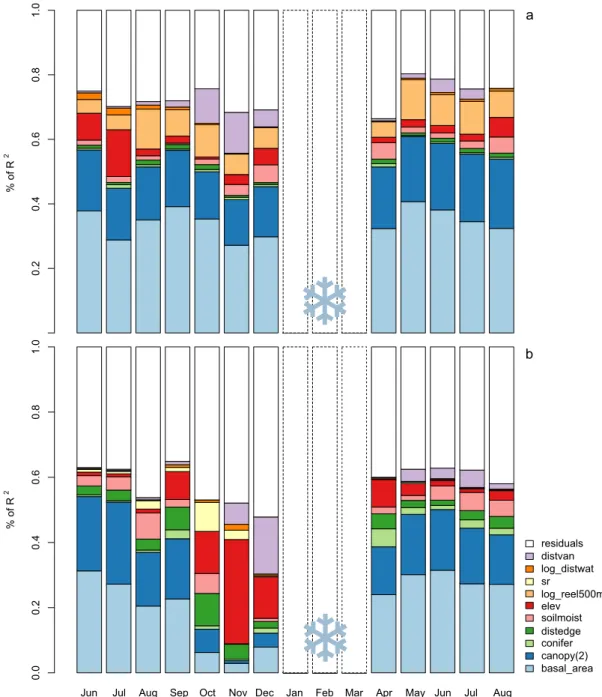
showed a consistent pattern across months with canopy cover and basal area contributing most to the modelfit and making up ca. two thirds of the overall modelR2, followed by relative elevation, elevation and dis-tance to lake Vänern (Fig. 4a). The latter is mainly contributing during autumn and early winter (October to December). Soil moisture con-tributed moderately mainly outside the warm season (November, De-cember, April).
The variation in relative elevation encountered in the study area had a generally strong effect on minimum temperatures (effect size: 4.18 °C in August 2015) and places with lower relative elevation (i.e. in depressions) had also lower minimum temperatures (Fig. S3, see Table S1 for raw model coefficients). Furthermore, cold temperatures were effectively buffered by increased forest basal area (effect size: 4.06 °C in August 2015) and canopy cover (1.60 °C) and lower elevation (−2.79 °C in July 2015). However, the lapse rate for minimum
temperatures was smaller in early autumn and spring (−2.3 °C km1in April) than in summer (−6.2 °C km−1in July 2015). The moderating effects of higher soil moisture (1.89 °C in December) and lesser distance to lake Vänern (−2.21 °C in October) were most pronounced in the cold season. Other explanatory variables had lower effects (see Table S1 and Fig. S3).
Monthly average maximum temperatures across the study area fluctuated between 22.7 °C in August 2015 and 2.3 °C in January 2016 (Fig. 2b). The variation among sites within a given month was large during the summer months (largest range of 21.4 °C in August) and decreased gradually towards the winter (smallest range of 3.8 °C in November). Again, the months with snow cover (January–March) were excluded from the models. Models performed best for summer months with the highest cross-validated R2of 0.59 but reached scores above 0.41 for all other months (Fig. 3b). The RMSE was generally higher Jun Jul Aug Sep Oct Nov Dec Jan Feb Mar Apr May Jun Jul Aug
residuals distvan log_distwat sr log_reel500m elev soilmoist distedge conifer canopy(2) basal_area
Fig. 4. Relative importance of predictors for models of monthly minimum temperature (a) and monthly maximum temperatures (b) across 12 months. Partial R2of variables sum up the
total R2of the full model (including all sites). basal_area = basal area, canopy(2) = canopy cover (square-root-transformed for minimum temperature models), conif = proportion of
conifers, distedge = distance to forest edge, soilmoist = soil moisture, elev = elevation, log_reel500m = (log) relative elevation in 500 m radius (only in models of minimum tem-perature), sr = solar radiation for the respective month (only in models of maximum temtem-perature), log_distwat = (log) distance to waterbodies, distvan = distance to lake Vänern. The snowflake marks months with snow cover (January–March), which were excluded from the models.
during summer months with the largest average cross-validated RMSE of 3.2 °C in August 2015 and the lowest RMSE of 0.6 °C in November (Fig. 3b).
Maximum temperatures were negatively correlated with minimum temperatures (places that become very hot get also very cold), except for the late autumn and winter months November, December and January where the pattern was the opposite (Fig. S5).
The relative importance of predictors for maximum temperatures was similar to the pattern for minimum temperatures, but with even larger influence of forest features from late spring to early autumn, making up to 80% of the explained variation (Fig. 4b). Outside the warm season, from October to December, physiographic features were the main contributors to overall R2(especially elevation, distance to lake Vänern and solar radiation). Distance to forest edge had a mod-erate influence across months, but slightly more during autumn and spring. Soil moisture contributed to about 20% to the modelfit.
Overall, basal area had the largest effect on lowering maximum temperatures (effect size: −9.70 °C in June 2016) followed by elevation (effect size: −5.61 °C in May) and canopy cover (effect size: −5.51 °C in June 2015, Fig. S4, see Table S2 for raw model coefficients). However, all these drivers show distinct seasonal patterns. For example, the inverse effects of basal area and canopy cover were stronger in summer than in autumn and spring. Soil moisture buffered high tem-peratures, particularly during the warm season (max. effect size in August 2015: 7.09 °C). Sites that were further away from lake Vänern also had slightly higher maximum temperatures during the summer (effect size: 3.94 °C in July 2016) but lower maximum temperatures during November and December. Solar radiation increased maximum temperatures significantly only during late summer and autumn (effect size: 4.89 °C in August 2015). Maximum temperatures decreased on average by 1.57 °C in August 2015 with increasing distance from forest edges and by 1.68 °C in April with increasing proportion of conifers.
3.2. MAP models
Correlation between soil moisture and TWI was weak (Spearman r = 0.30, df = 201, p < 0.001), moderate between canopy cover and remotely sensed basal area (r = 0.55, df = 201, p < 0.001), and strong between basal area and remotely sensed basal area (r = 0.84, df = 201, p < 0.001, Fig. S2).
When comparing the performance of OS with MAP models for minimum temperatures, the mean R2 of cross-validated models with
only remotely sensed predictors generally dropped compared to the OS models by 0.1 on average (Fig. 3a). Model error (RMSE) increased only less than 0.1 °C for 9 of 12 months, the largest increase in RMSE of 0.17 °C was observed in June and July 2016, and the lowest increase of less than 0.06 °C was observed in November (Fig. 3a). Predictions from the MAP models well matched the predictions from the OS models (Fig. 5a). The common slope across all months was slightly lower than one (0.82, p < 0.001, df = 1860, RMSE = 0.59), i.e. the predictions of the MAP models slightly overestimated the low and underestimated the high extremes of minimum temperatures for each month.
For maximum temperature mean R2of cross-validated models with only remotely sensed predictors were on average ca. 0.1 lower com-pared to the OS models, except in November, where MAP models even performed slightly better than the OS models (Fig. 3b). Average model fits above 0.4 could be obtained for 10 months with the highest R2
score of 0.5 in May. The average RMSE increased during the majority of months by about 0.2 °C, but had almost not changed during October to December (Fig. 3b). Predictions from the MAP models fairly well matched the predictions from the OS models (Fig. 5b), but compared to the OS models the accuracy of the MAP models was lower in the warmer months. The common slope across all months was slightly lower than one and also lower than the slope for minimum tempera-tures in the same analysis (0.75, p < 0.001, df = 1860, RMSE = 1.45), i.e. the predictions of the MAP model were less accurate for the low and high extremes of maximum temperatures for each month.
Remotely sensed basal area had the same effect as on-site measured basal area on both minimum and maximum temperatures (raw model coefficients provided in Tables S3 and S4). In contrast, the TWI as a soil moisture variable had no significant effect on models of minimum temperature, and buffered maximum temperatures in only half of the months (Tables S3 and S4).
The examples of microclimate maps inFig. 6 visualize the main corresponding climate-forcing factors for maximum temperature in summer (basal area) and autumn (elevation).
4. Discussion
4.1. Quantifying forest microclimate drivers across the seasons
The results of this study provide strong support for the notion that forest structure and composition and thus forest management had profound effects on the microclimatic landscape in a boreal forest
-5 -5 0 0 10 20 30 51 0 1 5 0
Tmin in ºC - fitted value of OS model
Tmin in ºC - fitted value of MAP
model
Tmin in ºC - fitted value of MAP
model
5 10 15 0 10
Tmin in ºC - fitted value of OS model
20 30 Apr May Jun Jul Aug Sep Oct Nov Dec Jun_16 Jul_16 Aug_16
Fig. 5. Fitted values of MAP models againstfitted values of on-site measurement (OS) models of monthly (a) minimum and (b) maximum temperatures. Mixed models with month as random effect (random intercept) revealed a common slope of 0.82 (p < 0.001, df = 1860, RMSE = 0.59) for minimum temperatures and 0.75 (p < 0.001, df = 1860, RMSE = 1.45) for maximum temperatures, i.e. the predictions of the MAP model overestimated the low and underestimated the high extremes of minimum temperatures for each month. OS models = models containing also on-site measured predictors. MAP models = models containing only remotely sensed predictors.
region. Forest density features were found to be the main drivers of local minimum and maximum temperatures during the warm season, whereas physiography (mainly elevation) had a larger relative in flu-ence on maximum temperatures in autumn and winter. The results were relatively similar in thefirst and second summer, suggesting that our models are robust.
Elevation, relative elevation and distance to lake Vänern were the most important physiographic climate-forcing factors, but effects fluc-tuated seasonally. The adiabatic decrease in temperature as a result of the atmospheric thermal stratification is known to differ depending on region, season and daytime (Dingman et al., 2013; Fridley, 2009;
Vercauteren et al., 2012). Elevation has often been reported to be a main microclimate driver in areas with complex terrain (Frey et al., 2016; Meineri et al., 2015; Vanwalleghem and Meentemeyer, 2009), whereas in our study it affected only maximum temperatures sub-stantially and only in the cold season, where environmental lapse rates were higher and recognizable even in an area outside steep topographic gradients (see also maps inFig. 6).
In agreement with earlier studies, we detected clear evidence of cold air pooling in terms of a positive relation between relative elevation and minimum temperatures (Ashcroft and Gollan, 2012;Meineri et al., 2015). This micro-meteorological phenomenon may have important implications for forestfloor biota, since it determines the occurrence
and depth of ground frost at the beginning and end of the growing season (Inouye, 2000). Despite that elevation and relative elevation were correlated (Spearman-|r| = 0.5, Fig. S2), they capture two dif-ferent phenomena (local vs. regional topography). Lake Vänern seemed to buffer low temperatures, especially in the autumn when this large water body cools down only slowly. The same buffering mechanism could be observed for maximum temperatures in summer. Solar ra-diation had a small effect on maximum temperatures, which may seem counterintuitive. However, we expected the influence of topographic shading to be moderate in a lowland landscape, which was probably even further declined due to overlapping effects of vegetation. In open landscape or in complex terrain, net solar radiation can be the domi-nant driver of spatial variation of high temperatures (Dingman et al., 2013;George et al., 2015;Maclean et al., 2016), but in lowland forests insolation of the ground is a function of both terrain and canopy shading. In northern Sweden, northern and southern slopes were found to have quite similar air temperatures but rather contrasting ground temperatures, perhaps due to wind effects and heat accumulation in the soil (Dahlberg et al., 2014). In our study area, solar radiation sig-nificantly increased maximum temperatures in late summer and au-tumn and had the largest relative influence in October, when sun angles were lower, and thus topographic shading more pronounced. The in-fluence of solar radiation became also much more noticeable in months
Fig. 6. Close-up of example temperature maps of maximum temperature in July (upper left) and maximum temperature in November (upper right) and the corresponding main climate drivers forest basal area (lower left) and elevation (lower right). All four panels show the same area, indicated inFig. 1.
with many clear days, which would explain, why its effect was sig-nificant in August 2015 (average cloud cover of 40 - 50%,SMHI, 2017) but not in August 2016, which was relatively more overcast (80 - 90% cloud cover). In high-latitude and in humid environments due to the time required for ground and water to heat up, daily temperatures peak long after the highest solar altitude and the summer solstice mostly precedes the warmest month(s) (Vercauteren et al., 2012). Additionally snow melt in spring and subsequent drying up of the soil can use up a substantial amount of radiation energy, before the air warms up. Therefore, alternative indices representing heat accumulation over time (perhaps even accounting for soil moisture and snow) may be more appropriate than instantaneous solar radiation.
Forest density, in terms of canopy cover and basal area, had a main influence on forest understory microclimate by buffering low and high extreme temperatures in the majority of months. Across the gradient of forest density, summer maximum temperatures differed by up to 12 °C and summer minimum temperatures by up to 4 °C. Maps of summer maximum temperatures reflect mainly gradients in canopy cover (shading from above) and basal area (shading from the side at high latitudes and low sun angles, Fig. 6). Even in November and April, when about half of the sites had average minimum temperatures below the frost point, forest basal area and canopy could increase low tem-peratures by 3 °C– enough to determine if a site experiences frost or not. Locally estimated, or remotely sensed, canopy cover was also found in other studies to be an important predictor for near-ground tem-peratures (Ashcroft and Gollan, 2012;George et al., 2015). Old-growth forest features in a montane Douglas-fir forest in central Oregon could decrease maximum spring temperatures by 2.5 °C (Frey et al., 2016). The effect sizes of forest density features were larger in our study, since we included also very young stands and forest clearings. However, excluding sites with young forest yielded similar results and only magnitude but not direction and significance of vegetation effects were dependent on the strong gradient from dense forest to open clear-cuts (results not shown). Several previous studies have included also the sub-canopy vegetation structure in microclimate models (Ashcroft and Gollan, 2012;Frey et al., 2016). However, in our study area and in managed boreal forests in general, the shrub layer is often missing and was therefore disregarded in this study.
In our study, forest edge effects were mainly noticeable for max-imum temperatures. This is consistent with prior findings (Vanwalleghem and Meentemeyer, 2009) and may be caused by strong shade gradients during daytime. In addition, during daytime cooler forest air can“drain” at forest edges, decreasing further the buffering capacity of dense forests against high temperatures (Baker et al., 2014;
Geiger et al., 2012). Forest fragmentation is therefore predicted to in-tensify landscape warming trends (Ewers and Banks-Leite, 2013;
Vanwalleghem and Meentemeyer, 2009) and may cause extra harm to understory biodiversity, that depends on cooler forest microclimates. During the cold season, forests can be slightly warmer than open areas due to reduced wind speed and low albedo (see the positive effect of basal area on maximum temperatures in December, Fig. S4, and
Latimer and Zuckerberg, 2016). However, the same “leaking” effect also causes fragmented forests to be colder during the day than con-tinuous forests, losing for example the ability to provide sheltered mi-croclimates for overwintering passerines (Latimer and Zuckerberg, 2016).
Forest composition played a less dominant role in our study, though sites with more conifers had slightly lower minimum temperatures in July and August 2015 (i.e. less than 1 °C, Fig. S3) and lower maximum temperatures in April (almost 2 °C across the observed gradient, Fig. S3). Compared to deciduous trees, the canopy of conifer stands has often larger gaps and is therefore less effective in retaining heat at night during summer. On the contrary, in spring before foliation of deciduous trees, conifers provide more shade, and can therefore decrease daily maximum temperatures on the forestfloor. Thus not only litter fall, soil properties and light (Rydin et al., 1999), but also temperature profiles
across the year might differ between coniferous, mixed and deciduous stands. Additionally, pine-dominated stands have a less dense canopy cover letting in more light compared to darker spruce-dominated stands and are thus expected to create different microclimates. However, these differences are less pronounced in younger forest patches, and in-cluding the identity of pine and spruce in our OS models did not explain more of the variation in temperatures (results not shown).
Boreal forests occur in latitudes with distinct seasonality in light, temperature, precipitation and vegetation phenology, and therefore also in microclimatic variability. In our study area, the spatial variation in microclimate was more pronounced for maximum temperatures and during the warm season, whereas in the cold season the maximum temperatures were very similar across the landscape. In autumn the evenness of maximum temperatures across space is caused by strong winds, while during the winter it is caused by rather low solar heating capacity and frequent snow cover (mainly in January and February).
Although absolute temperature differences across the landscape are largest in clear summer days, microclimatic differences may be biolo-gically more relevant during spring nights, when only small tempera-ture variations may be associated with frost events– one of the main limiting factors for ground-dwelling biota. Since the relevance of a microclimatic variable depends on the studied organism(s) or process (Hylander et al., 2015), we modelled 24 different variables to choose from (minimum and maximum temperatures of 12 months) and which can be further translated into other bioclimatic variables, e.g. growing degree days or annual climatic variability. By modelling average ex-treme temperatures separately over 12 months, we could also study the temporal dynamic of the effects of landscape physiography and vege-tation on near-ground temperatures. This temporal variation in effects and importance of microclimatic drivers seems to be common, and has been found when modelling seasonal, daily or hourly temperatures separately (Ashcroft and Gollan, 2013a;George et al., 2015;Maclean et al., 2016).
It is noteworthy, that the relationship of minimum and maximum temperatures also changed throughout the year, with negative corre-lations from March to September and positive correlation between November and January (Fig. S5). In other words, sites that become hot during the day, get also very cold during the night (March to September). This was most pronounced for clear-cuts and young stands that lack a buffering vegetation layer. During the cold season, when maximum temperatures were more uniform across the study area and also more influenced by physiographic features, cold sites are sistently cold during day and night. Hence, drawing biological con-clusions depends on the organisms of focus and their physiological re-quirements across the year. Many herbs in boreal forests overwinter belowground as roots, rhizomes or seeds, or are covered by snow, protecting them against extreme frost. Therefore winter microclimates per se may be less biologically relevant for them. Conversely, local temperatures during the winter may correlate with the timing of snowmelt, which in turn is a crucial point for below or above ground biota.
4.2. Model limitations
Our model fits were generally good and only slightly lower for maximum temperature models during the cold months, when the temperature variation across loggers was very low (seeFig. 2). This is during times when regional air masses control temperatures and the low sun does not provide enough energy to create heterogeneous warming of the landscape. The unexplained variance in the other monthly models likely resulted from omitting other (unavailable) cli-mate drivers, ignoring interactions among clicli-mate-forcing factors due to the limited sample size, and the within-site heterogeneity of some climate-forcing factors. A particular difficulty is the extreme high spa-tial variability of summer maximum temperatures on the ground due to patchiness of sunbeams and shades created by the forest canopy. This
may have resulted in non-representative temperature measurements for some sites, which could only insufficiently be explained by environ-mental factors at a 25 m resolution, leading to comparably large model errors up to 3 °C (Fig. 3b). However, the absolute differences (range) of
summer maximum temperatures were also particularly high (up to 20 °C,Fig. 2b), and even with higher model errors relative predictions may still hold. Similarly, Ashcroft and Gollan (2013b) found that within-site variation of high temperatures varied a lot resulting in lower model fits, whereas within-site variation of cold temperatures was negligible. Reliability and representativity of air temperature mea-surements could be improved by applying more sophisticated (double) radiation shields, that for example do not trap heat convection and radiation from the ground (Holden et al., 2013; Körner and Hiltbrunner, 2017).
4.3. MAP models
We could successfully produce reliable high-resolution (25 m) maps of minimum and maximum temperatures for 12 months with reason-ably low model uncertainty. Modelfits of the MAP models were slightly lower than those of the on-site (OS) models, which can be attributed to inaccurate mapped predictors for soil moisture and forest features or to disregarded predictors, which were lacking in a mapped form (distance to forest edge, proportion of conifers). Modelling of forest microclimate is challenging due to unquantified small-scale variation of light, tem-perature and humidity at the forestfloor and missing precisely mapped and up-to-date predictors of the canopy and the ground vegetation. The newly available laser-scanning products (here basal area) succeeded though to reflect local canopy cover and field-based basal area (high correlations: 0.55 and 0.84). However, particularly for managed forests up-to-date vegetation maps are desirable, which capture the results of management activities (e.g. from regular laser scanning or provision of stand information by forest owners). For forests with a larger deciduous component, separate estimates for canopy cover before and after tree leafing are needed. In general, methods need to be developed and re-fined to include remote sensing data into ecological and microclimate modelling (He et al., 2015;Lenoir et al., 2017;Turner et al., 2003).
4.4. Implications for management and conservation
Climate warming leads to species migration and extinctions (Settele et al., 2014;Thomas et al., 2004;Thuiller et al., 2008,2005). The role of microclimate in climate driven range shifts has often been high-lighted as having the potential to facilitate species survival in micro-refugia or establishment in stepping stone habitats (Hannah et al., 2014;Keppel et al., 2012;Lenoir et al., 2017;Rull, 2009). By providing microclimate maps, it will be possible to identify and protect areas with exceptional microclimate and of high conservation value (e.g. sites that are warmer or colder than the surrounding matrix, sites that are de-coupled from the regional climate, or sites with slower rate of warming).
Our study demonstrated that forest features dominated over phy-siographic climate-forcing factors in a boreal forest landscape. As a consequence, forest management has major control on shaping the climatic environment (D’Odorico et al., 2013;Frey et al., 2016). Forest management actions could involve the creation of strong temperature gradients within an area, increasing landscape heterogeneity, by for example having less dense forests on south/west facing slopes and dense forests on north/east facing slopes. Depressions, typically char-acterized by the effect of cold air pooling can be kept cool during day by maintaining a dense forest stand. Simultaneously dense forests can moderate steep microclimatic gradients created by topography and maintaining continuous stands on topographically exposed places (e.g. by selective logging vs. clearing) can help in avoiding further damage by wind, frost and out-drying. Additional ways to intentionally modify forest microclimate include adjusting the proportion of conifers and
deciduous trees and managing the age structure of forest stands.Frey et al. (2016)revealed the improved cooling effect of old-growth forests
with a high vertical complexity compared to simplified plantations. Finally due to the large effects of forest edges on maximum tempera-tures in forests (Fig. S4), fragmentation and a high density of forest edges due to the intensive forestry may impede harmful effects of global climate warming, and the spatial arrangement and size of these clear-ings need careful planning (Dynesius et al., 2008). At the same time, mature forests positively influence conditions on adjacent regenerating forest patches and various forms of retention forestry have been sug-gested to “promote re-colonization of mature-forest species” (Baker et al., 2014).
4.5. Conclusions
Future attempts to downscale climate data should incorporate ve-getation features, especially in human-modified forest landscapes. Standardized weather stations could for example add instrumentation in adjacent forests to increase the number of systematic measurements also over a longer time period (De Frenne and Verheyen, 2015). In this study, we showed that the influence and effects of physiographic and biophysical climate-forcing factors change seasonally. This calls for inclusion of the temporal aspect in microclimate studies. Further, better mapped climate-forcing factors are needed in order to be able to pro-duce robust microclimate maps (Lenoir et al., 2017). At last, in order to advance our understanding of microclimate variation as well as to produce biologically meaningful climate grids, substantially more col-laborative research by ecologists and meteorologists is required.
Data accessibility
The produced climate grids are available from the Dryad Digital Repository:https://doi.org/10.5061/dryad.hv044.
Acknowledgements
This research was funded by a FORMAS project grant 2014-530 [to KH]. We thank William Lidberg for help with Whitebox, Sveaskog and Bergvik for provision of forest data and permission to work on their property and Anton Hammarström, Anna Hessel Hassel, Valentin Journe, Lisa Sandberg, Ros van der Spoel and Lina Widenfalk for as-sisting duringfield work. We also thank Mick Ashcroft and Jonathan Lenoir for valuable comments and suggestions on the manuscript.
Appendix A. Supplementary data
Supplementary material related to this article can be found, in the online version, at doi:https://doi.org/10.1016/j.agrformet.2017.12. 252
References
Aalto, J., Riihimäki, H., Meineri, E., Hylander, K., Luoto, M., 2017. Revealing topocli-matic heterogeneity using meteorological station data. Int. J. Climatol.http://dx.doi. org/10.1002/joc.5020.
Abràmoff, M.D., Magalhães, P.J., Ram, S.J., 2004. Image processing with Image. J. Biophotonics Int. 11, 36–41.http://dx.doi.org/10.1117/1.3589100.
Anderson, J.M., 1991. The effects of climate change on decomposition processes in grassland and coniferous forests. Ecol. Appl. 1, 326–347.
Ashcroft, M.B., French, K.O., Chisholm, L.a., 2011. An evaluation of environmental fac-tors affecting species distributions. Ecol. Model. 222, 524–531.http://dx.doi.org/10. 1016/j.ecolmodel.2010.10.003.
Ashcroft, M.B., Gollan, J.R., 2013a. Moisture, thermal inertia, and the spatial distribu-tions of near-surface soil and air temperatures: understanding factors that promote microrefugia. Agric. For. Meteorol. 176, 77–89.http://dx.doi.org/10.1016/j. agrformet.2013.03.008.
Ashcroft, M.B., Gollan, J.R., 2013b. The sensitivity of topoclimatic models tofine-scale microclimatic variability and the relevance for ecological studies. Theor. Appl. Climatol. 114, 281–289.http://dx.doi.org/10.1007/s00704-013-0841-0. Ashcroft, M.B., Gollan, J.R., 2012. Fine-resolution (25 m) topoclimatic grids of
near-surface (5 cm) extreme temperatures and humidities across various habitats in a large (200 x 300 km) and diverse region. Int. J. Climatol. 32, 2134–2148.http://dx.doi. org/10.1002/joc.2428.
Ashcroft, M.B., Gollan, J.R., Warton, D.I., Ramp, D., 2012. A novel approach to quantify and locate potential microrefugia using topoclimate, climate stability, and isolation from the matrix. Glob. Chang. Biol. 18, 1866–1879.http://dx.doi.org/10.1111/j. 1365-2486.2012.02661.x.
Baker, T.P., Jordan, G.J., Steel, E.A., Fountain-Jones, N.M., Wardlaw, T.J., Baker, S.C., 2014. Microclimate through space and time: microclimatic variation at the edge of regeneration forests over daily, yearly and decadal time scales. For. Ecol. Manage. 334, 174–184.http://dx.doi.org/10.1016/j.foreco.2014.09.008.
Beven, K.J., Kirkby, M.J., 1979. A physically based, variable contributing area model of basin hydrology. Hydrol. Sci. Bull. 24, 43–69.http://dx.doi.org/10.1080/ 02626667909491834.
Bonan, G.B., Shugart, H.H., 1989. Ecological processes in boreal forests. Annu. Rev. Ecol. Syst. 20, 1–28.
Chen, J., Franklin, J.F., 1997. Growing-season microclimate variability within an old-growth Douglas-fir forest. Clim. Res. 8, 21–34.http://dx.doi.org/10.3354/cr008021. Chen, J., Franklin, J.F., Spies, T.A., 1993. Contrasting microclimates among clearcut,
edge, and interior of old-growth Douglas-fir forest. Agric. For. Meteorol. 63, 219–237.
http://dx.doi.org/10.1016/0168-1923(93)90061-L.
Chen, J., Saunders, S.C., Crow, T.R., Naiman, R.J., Brosofske, K.D., Mroz, G.D., Brookshire, B.L., Franklin, J.F., 1996. Microclimate in forest ecosystem and land-scape. Ecology 49.
D’Odorico, P., He, Y., Collins, S., De Wekker, S.F.J., Engel, V., Fuentes, J.D., 2013. Vegetation-microclimate feedbacks in woodland-grassland ecotones. Glob. Ecol. Biogeogr. 22, 364–379.http://dx.doi.org/10.1111/geb.12000.
Dahlberg, C.J., Ehrlén, J., Hylander, K., 2014. Performance of forest bryophytes with different geographical distributions transplanted across a topographically hetero-geneous landscape. PLoS One 9.http://dx.doi.org/10.1371/journal.pone.0112943. De Frenne, P., Rodríguez-Sánchez, F., Coomes, D.A., Baeten, L., Verstraeten, G., Vellend,
M., Bernhardt-Römermann, M., Brown, C.D., Brunet, J., Cornelis, J., Decocq, G.M., Dierschke, H., Eriksson, O., Gilliam, F.S., Hédl, R., Heinken, T., Hermy, M., Hommel, P., Jenkins, M.A., Kelly, D.L., Kirby, K.J., Mitchell, F.J.G., Naaf, T., Newman, M., Peterken, G., Petrík, P., Schultz, J., Sonnier, G., Van Calster, H., Waller, D.M., Walther, G.-R., White, P.S., Woods, K.D., Wulf, M., Graae, B.J., Verheyen, K., 2013. Microclimate moderates plant responses to macroclimate warming. Proc. Natl. Acad. Sci. U. S. A. 110, 18561–18565.http://dx.doi.org/10.1073/pnas.1311190110.
De Frenne, P., Verheyen, K., 2015. Weather stations lack forest data. Science (80-.) 351, 234.
Dingman, J.R., Sweet, L.C., McCullough, I., Davis, F.W., Flint, A., Franklin, J., Flint, L.E., 2013. Cross-scale modeling of surface temperature and tree seedling establishment in mountain landscapes. Ecol. Process. 2, 30. http://dx.doi.org/10.1186/2192-1709-2-30.
Dobrowski, S.Z., 2011. A climatic basis for microrefugia: the influence of terrain on cli-mate. Glob. Chang. Biol. 17, 1022–1035.http://dx.doi.org/10.1111/j.1365-2486. 2010.02263.x.
Dynesius, M., Åström, M., Nilsson, C., 2008. Microclimatic buffering by logging residues and forest edges reduces clear-cutting impacts on forest bryophytes. Appl. Veg. Sci. 11, 345–354.http://dx.doi.org/10.3170/2008-7-18457.
Ewers, R.M., Banks-Leite, C., 2013. Fragmentation impairs the microclimate buffering effect of tropical forests. PLoS One 8.http://dx.doi.org/10.1371/journal.pone. 0058093.
Frey, S.J.K., Hadley, A.S., Johnson, S.L., Schulze, M., Jones, J.A., Betts, M.G., 2016. Spatial models reveal the microclimatic buffering capacity of old-growth forests. Sci. Adv. 2.
Fridley, J.D., 2009. Downscaling climate over complex terrain: highfinescale (< 1000 m) spatial variation of near-ground temperatures in a montane forested landscape (Great Smoky Mountains). J. Appl. Meteorol. Climatol. 48, 1033–1049.http://dx.doi.org/ 10.1175/2008JAMC2084.1.
Geiger, R., Aron, R.H., Todhunter, P., 2012. The Climate Near the Ground, 5th ed. Springer Science & Business Media.
George, A.D., Thompson, F.R., Faaborg, J., 2015. Using LiDAR and remote microclimate loggers to downscale near-surface air temperatures for site-level studies. Remote Sens. Lett. 6, 924–932.http://dx.doi.org/10.1080/2150704X.2015.1088671.
Giesler, R., Högberg, M., Högberg, P., 1998. Soil chemistry and plants in fennoscandian boreal forest as exemplified by a local gradient. Ecology 79, 119–137.
Grömping, U., 2006. Relative importance for linear regression in R: the package relaimpo. J. Stat. Softw. 17, 139–147.http://dx.doi.org/10.1016/j.foreco.2006.08.245. Hannah, L., Flint, L., Syphard, A.D., Moritz, M.A., Buckley, L.B., Mccullough, I.M., 2014.
Fine-grain modeling of species’ response to climate change : holdouts, stepping-stones, and microrefugia. Trends Ecol. Evol. 29, 390–397.http://dx.doi.org/10. 1016/j.tree.2014.04.006.
He, K.S., Bradley, B.A., Cord, A.F., Rocchini, D., Tuanmu, M.N., Schmidtlein, S., Turner, W., Wegmann, M., Pettorelli, N., 2015. Will remote sensing shape the next generation of species distribution models? Remote Sens. Ecol. Conserv. 1, 4–18.http://dx.doi. org/10.1002/rse2.7.
Holden, Z.A., Klene, A.E., Keefe, R.F., Moisen, G.G., 2013. Design and evaluation of an inexpensive radiation shield for monitoring surface air temperatures. Agric. For. Meteorol. 180, 281–286.http://dx.doi.org/10.1016/j.agrformet.2013.06.011. Hylander, K., Ehrlén, J., Luoto, M., Meineri, E., 2015. Microrefugia: Not for everyone.
Ambio 44, 60–68.http://dx.doi.org/10.1007/s13280-014-0599-3.
Hägglund, B., Lundmark, J.E., 1981. Handledning i bonitering med Skogskhögskolans boniteringssystem. Jönköping, Sweden..
Inouye, D.W., 2000. The ecological and evolutionary significance of frost in the context of climate change. Ecol. Lett. 3, 457–463.http://dx.doi.org/10.1046/j.1461-0248.
2000.00165.x.
Keppel, G., Van Niel, K.P., Wardell-johnson, G.W., Yates, C.J., Byrne, M., Mucina, L., Schut, A.G.T., Hopper, S.D., Franklin, S.E., 2012. Refugia: identifying and under-standing safe havens for biodiversity under climate change. Glob. Ecol. Biogeogr. 21, 393–404.http://dx.doi.org/10.1111/j.1466-8238.2011.00686.x.
Körner, C., Hiltbrunner, E., 2017. The 90 ways to describe plant temperature. Perspect. Plant Ecol. Evol. Syst. 1–6.http://dx.doi.org/10.1016/j.ppees.2017.04.004.
Lantmäteriet, 2009. GSD-Elevation Data, Grid 2+ [WWW Document]. URL: http:// www.lantmateriet.se/globalassets/kartor-och-geografisk-information/hojddata/pro-duktbeskrivningar/eng/e_grid2_plus.pdf (Accessed 9.12.17)..
Larsson, S., Nilsson, L., Persson, A., André, P., Eriksson, J., Nilsson, M., Olsson, H., Lysell, G., 2016. Skogliga skattningar från laserdata (“Forest estimates from laserdata”), Skogsstyrelsens Meddelande. Jönköping, Sweden..
Latimer, C.E., Zuckerberg, B., 2016. Forest fragmentation alters winter microclimates and microrefugia in human-modified landscapes. Ecogr. (Cop.) 158–170.http://dx.doi. org/10.1111/ecog.02551.
Lenoir, J., Graae, B.J., Aarrestad, P.A., Alsos, I.G., Armbruster, W.S., Austrheim, G., Bergendorff, C., Birks, H.J.B., Bråthen, K.A., Brunet, J., Bruun, H.H., Dahlberg, C.J., Decocq, G., Diekmann, M., Dynesius, M., Ejrnæs, R., Grytnes, J.A., Hylander, K., Klanderud, K., Luoto, M., Milbau, A., Moora, M., Nygaard, B., Odland, A., Ravolainen, V.T., Reinhardt, S., Sandvik, S.M., Schei, F.H., Speed, J.D.M., Tveraabak, L.U., Vandvik, V., Velle, L.G., Virtanen, R., Zobel, M., Svenning, J.C., 2013. Local tem-peratures inferred from plant communities suggest strong spatial buffering of climate warming across Northern Europe. Glob. Chang. Biol. 19, 1470–1481.http://dx.doi. org/10.1111/gcb.12129.
Lenoir, J., Hattab, T., Pierre, G., 2017. Climatic microrefugia under anthropogenic cli-mate change: implications for species redistribution. Ecogr. (Cop.) 40, 253–266.
http://dx.doi.org/10.1111/ecog.02788.
Lindsay, J.B., 2016a. Whitebox GAT: a case study in geomorphometric analysis. Comput. Geosci. 95, 75–84.http://dx.doi.org/10.1016/j.cageo.2016.07.003.
Lindsay, J.B., 2016b. Efficient hybrid breaching-filling sink removal methods for flow path enforcement in digital elevation models. Hydrol. Process. 30, 846–857.http:// dx.doi.org/10.1002/hyp.10648.
Lookingbill, T.R., Urban, D.L., 2003. Spatial estimation of air temperature differences for landscape-scale studies in montane environments. Agric. For. Meteorol. 114, 141–151.http://dx.doi.org/10.1016/S0168-1923(02)00196-X.
Maclean, I.M.D., Suggitt, A.J., Wilson, R.J., Duffy, J.P., Bennie, J.J., 2016. Fine-scale climate change: modelling spatial variation in biologically meaningful rates of warming. Glob. Chang. Biol. 1–13.http://dx.doi.org/10.1111/gcb.13343. Means, J.E., Acker, S.A., Fitt, B.J., Renslow, M., Emerson, L., Abstract, C.J.H., 2000.
Predicting forest stand characteristics with airborne scanning lidar. Photogramm. Eng. Remote Sens. 66, 1367–1371.http://dx.doi.org/10.1016/S0034-4257(01) 00290-5.
Meineri, E., Dahlberg, C.J., Hylander, K., 2015. Using Gaussian Bayesian Networks to disentangle direct and indirect associations between landscape physiography, en-vironmental variables and species distribution. Ecol. Modell. 313, 127–136.http:// dx.doi.org/10.1016/j.ecolmodel.2015.06.028.
Meineri, E., Hylander, K., 2016. Fine-grain, large-domain climate models based on cli-mate station and comprehensive topographic information improve microrefugia de-tection. Ecogr. (Cop.) 40, 1003–1013.http://dx.doi.org/10.1111/ecog.02494. Nilsson, M.C., Wardle, D.A., 2005. Understory vegetation as a forest ecosystem driver:
evidence from the northern Swedish boreal forest. Front. Ecol. Environ. 3, 421–428.
http://dx.doi.org/10.1890/1540-9295(2005)003[0421:UVAAFE]2.0.CO;2. Östlund, L., Zackrisson, O., Axelsson, A.-L., 1997. The history and transformation of a
Scandinavian boreal forest landscape since the 19th century. Can. J. For. Res. 27, 1198–1206.http://dx.doi.org/10.1139/x97-070.
R Core Team, 2012. R: A Language and Environment for Statistical Computing. R Foundation for Statistical Computing, Vienna.
Rosenberg, N.J., 1974. Microclimate: The Biological Environment. Wiley-Interscience Publication, John Wiley & Sons, New York.
Ruckstuhl, K.E., Johnson, E.A., Miyanishi, K., 2008. Introduction. The boreal forest and global change. Philos. Trans. R. Soc. Lond. B Biol. Sci. 363, 2245–2249.http://dx.doi. org/10.1098/rstb.2007.2196.
Rull, V., 2009. Microrefugia J. Biogeogr. 36, 481–484. http://dx.doi.org/10.1111/j.1365-2699.2008.02023.x.
Rydin, H., Snoeijs, P., Diekmann, M. (Eds.), 1999. Swedish Plant Geography. Uppsala.
Settele, J., Scholes, R.J., Betts, R.A., Bunn, S., Leadley, P., Nepstad, D., Overpeck, J.T., Toboada, M.A., 2014. Terrestrial and inland water systems. In: Field, C.B., Barros, V.R., Dokken, D.J., Mach, K.J., Mastrandrea, M.D., Bilir, T.E., Chatterjee, M., Ebi, K.L., Estrada, Y.O., Genova, R.C., Girma, B., Kissel, E.S., Levy, A.N., MacCracken, S., Mastrandrea, P.R., White, L.L. (Eds.), Climate Change 2014: Impacts, Adaptation, and Vulnerability. Part A: Global and Sectoral Aspects. Contribution of Working Group II to the Fifth Assessment Report of the Intergovernmental Panel on Climate Change. Cambridge University Press, Cambridge, United Kingdom and New York, NY, USA, pp. 271–359 doi:31 March 2014.
Sjörs, H., et al., 1965. The plant cover of Sweden. A study dedicated to G. Einar Du Rietz on his 70th birthday by his pupils. Acta Phytogeogr. Suec. 50, 1–314.
SLU, 2017. Climate. Department of Soil and Environment, Swedish University of Agricultural Sciences [WWW Document]. URL http://www-markinfo.slu.se/eng/ climate/klimat.html (Accessed 5.16.17)...
SMHI, 2017. Swedish Meteorological and Hydrological Institute. Klimatdata. Database: Dataserier med normalvärden för perioden 1961–1990. [WWW Document]. URL https://www.smhi.se/klimatdata/ (Accessed 3.20.17)..
Sørensen, R., Zinko, U., Seibert, J., 2006. On the calculation of the topographic wetness index: evaluation of different methods based on field observations. Hydrol. Earth Syst. Sci. 10, 101–112.http://dx.doi.org/10.5194/hess-10-101-2006.
Thomas, C.D., Cameron, A., Green, R.E., Bakkenes, M., Beaumont, L.J., Collingham, Y.C., Erasmus, B.F.N., De Siqueira, M.F., Grainger, A., Hannah, L., Hughes, L., Huntley, B., Van Jaarsveld, A.S., Midgley, G.F., Miles, L., Ortega-Huerta, M.A., Peterson, A.T., Phillips, O.L., Williams, S.E., 2004. Extinction risk from climate change. Nature 427, 145–148.http://dx.doi.org/10.1038/nature02121.
Thuiller, W., Albert, C., Araújo, M.B., Berry, P.M., Cabeza, M., Guisan, A., Hickler, T., Midgley, G.F., Paterson, J., Schurr, F.M., Sykes, M.T., Zimmermann, N.E., 2008. Predicting global change impacts on plant species’ distributions: future challenges. Perspect. Plant Ecol. Evol. Syst. 9, 137–152.http://dx.doi.org/10.1016/j.ppees.2007. 09.004.
Thuiller, W., Lavorel, S., Araujo, M.B., Sykes, M.T., Prentice, I.C., 2005. Climate change threats to plant diversity in Europe. Proc. Natl. Acad. Sci. U. S. A. 102, 8245–8250.
http://dx.doi.org/10.1073/pnas.0409902102.
Turner, W., Spector, S., Gardiner, N., Fladeland, M., Sterling, E., Steininger, M., 2003. Remote sensing for biodiversity science and conservation. Trends Ecol. Evol. 18, 306–314.http://dx.doi.org/10.1016/S0169-5347(03)00070-3.
Vanwalleghem, T., Meentemeyer, R.K., 2009. Predicting forest microclimate in hetero-geneous landscapes. Ecosystems 1158–1172. http://dx.doi.org/10.1007/s10021-009-9281-1.
Vercauteren, N., Destouni, G., Dahlberg, C.J., Hylander, K., 2012. Fine-resolved, near-coastal spatiotemporal variation of temperature in response to insolation. J. Appl. Meteorol. Climatol. 52, 1208–1220.http://dx.doi.org/10.1175/JAMC-D-12-0115.1. Walther, G.R., Roques, A., Hulme, P.E., Sykes, M.T., Pyšek, P., Kühn, I., Zobel, M., Bacher, S., Botta-Dukát, Z., Bugmann, H., Czúcz, B., Dauber, J., Hickler, T., Jarošík, V., Kenis, M., Klotz, S., Minchin, D., Moora, M., Nentwig, W., Ott, J., Panov, V.E., Reineking, B., Robinet, C., Semenchenko, V., Solarz, W., Thuiller, W., Vilà, M., Vohland, K., Settele, J., 2009. Alien species in a warmer world: risks and opportunities. Trends Ecol. Evol. 24, 686–693.http://dx.doi.org/10.1016/j.tree.2009.06.008.
Zimmermann, N.E., Yoccoz, N.G., Edwards, T.C., Meier, E.S., Thuiller, W., Guisan, A., Schmatz, D.R., Pearman, P.B., 2009. Climatic extremes improve predictions of spatial patterns of tree species. Proc. Natl. Acad. Sci. U. S. A. 106, 19723–19728.http://dx. doi.org/10.1073/pnas.0901643106.