T E C H N I C A L R E P O R T
Open Access
GEOMAGIA50.v3: 2. A new paleomagnetic
database for lake and marine sediments
Maxwell C Brown
1*, Fabio Donadini
2, Andreas Nilsson
3,4, Sanja Panovska
5, Ute Frank
1,
Kimmo Korhonen
6, Maximilian Schuberth
7,8, Monika Korte
1and Catherine G Constable
5Abstract
Background: GEOMAGIA50.v3 for sediments is a comprehensive online database providing access to published paleomagnetic, rock magnetic, and chronological data obtained from lake and marine sediments deposited over the past 50 ka. Its objective is to catalogue data that will improve our understanding of changes in the geomagnetic field, physical environments, and climate.
Findings: GEOMAGIA50.v3 for sediments builds upon the structure of the pre-existing GEOMAGIA50 database for magnetic data from archeological and volcanic materials. A strong emphasis has been placed on the storage of geochronological data, and it is the first magnetic archive that includes comprehensive radiocarbon age data from sediments. The database will be updated as new sediment data become available.
Conclusions: The web-based interface for the sediment database is located at http://geomagia.gfz-potsdam.de/ geomagiav3/SDquery.php. This paper is a companion to Brown et al. (Earth Planets Space doi:10.1186/s40623-015-0232-0, 2015) and describes the data types, structure, and functionality of the sediment database.
Keywords: Geomagnetism; Paleomagnetism; Sediment magnetism; Rock magnetism; Environmental magnetism; Database; GEOMAGIA50
Findings
Introduction
The aim of the GEOMAGIA50 database is to allow easy access to paleomagnetic data from the past 50 ka. Previous versions of the database (Donadini et al. 2006; Korhonen et al. 2008) stored palaeomagnetic data from archeolog-ical materials and lavas alone; however, paleomagnetic, rock magnetic, and chronological data from sediments deposited over the past 50 ka have broad applications across the geosciences. These include understanding past changes in the geomagnetic field, physical environments, climate, and anthropogenic impact.
In a companion paper (Brown et al. 2015), the lat-est modifications to the general structure of the GEO-MAGIA50 database and more specific changes to the archeo/volcanic database are described. This paper
*Correspondence: [email protected]
1GFZ German Research Centre for Geosciences, Telegrafenberg, 14473 Potsdam, Germany
Full list of author information is available at the end of the article
addresses the scientific rationale, design, and function of the newly implemented sediment database.
Paleomagnetic data from sediments complement the wealth of data from archeological and volcanic materials covering the same period already stored within the GEO-MAGIA50 database (Brown et al. 2015). Furthermore, the amount of paleomagnetic data from archeological mate-rials and lavas decreases greatly prior to 2 ka (see Brown et al. 2015; Donadini et al. 2009). Paleomagnetic data from sediments are therefore essential to our understanding of the temporal and spatial evolution of the geomagnetic field over longer time scales. In addition, the inclusion of rock magnetic and chronological data from sediments in GEOMAGIA50 expands the range of scientific problems that can be addressed by the database.
The quasi-continuous nature of sediments makes them an attractive source of information about temporal changes in the geomagnetic field. They augment archeo-magnetic and volcanic data, which provide only spot readings of the paleomagnetic field and are often sparsely distributed in time (e.g., Guyodo and Valet 1999a). The
© 2015 Brown et al.; licensee Springer. This is an Open Access article distributed under the terms of the Creative Commons Attribution License (http://creativecommons.org/licenses/by/4.0), which permits unrestricted use, distribution, and reproduction in any medium, provided the original work is properly credited.
joint analysis of sediment and archeomagnetic and/or lava data allows the resolution of a greater degree of complex-ity in field behavior (e.g., Korte and Constable 2005). This is true for not only the past 50 ka, but in the case of lavas, over other geomagnetically interesting times, such as during reversals (e.g., Brown et al. 2013; Coe and Glen 2004).
In recent years, paleomagnetic data from sediments have been incorporated into empirical models of the Holocene geomagnetic field (e.g., Korte and Constable 2005; Korte et al. 2009, 2011; Licht et al. 2013; Nilsson et al. 2014; Panovska 2012). Encouragingly, Holocene geo-magnetic field models generate globally consistent time-averaged structures; however, in some studies, low-quality paleomagnetic data from sediments and/or erroneous age models can result in temporal ambiguities between records and therefore a distorted picture of the time-varying geomagnetic field. Providing more comprehen-sive data will enable a rigorous assessment of the factors that may influence these records and allow more realistic uncertainties to be assigned.
To learn more about the mechanisms that generate the geomagnetic field, it is necessary to understand variations in the field over different time scales. Holocene geomag-netic field variations cover only part of the range of field behavior seen throughout geological time (Figure 1). The period between 50 ka and the present contains a wealth of geomagnetic variability that we understand only in part. Sediments deposited over this time have the advantage of being within the limits of radiocarbon dating, as well as being suitable for dating by other chronological methods (e.g.,δ18O dating, tephra chronology, and varve counting). Although the limit of radiocarbon dating is approximately 62 ka (Plastino et al. 2001), the most recent calibration curves for variations in atmospheric carbon through time end at 50 ka (Reimer 2013).
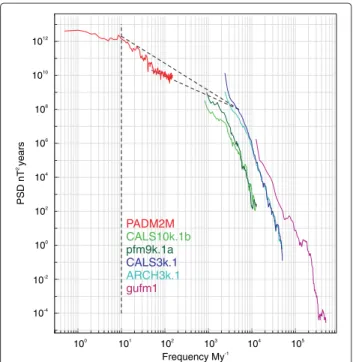
The power spectrum of geomagnetic dipole moment variations allows us to investigate the time necessary to average the geomagnetic field to obtain a stable time-average (if this exists). In addition, the distribution of power over the full range of frequencies applicable to the geomagnetic field has important statistical proper-ties that can be compared with the output of numerical dynamo simulations (e.g., Davies and Constable 2014; Driscoll and Olson 2009; Olson et al. 2012; Sakuraba and Hamano 2007). This spans from measurements of short-term variations of the present day field, through satellite missions such as Swarm (Olsen et al. 2013) and observa-tory data (Reay et al. 2011), to paleomagnetic observations of superchrons, such as the Cretaceous Normal Super-chron (e.g., Granot et al. 2012; Tarduno et al. 2001; Tauxe and Staudigel 2004). Ziegler and Constable (2011) investi-gated the power spectrum over the last 2 Ma (see Figure 1 for a composite spectrum derived from various sources
Frequency My-1 101 100 102 103 104 105 sr a e y T n D S P 2 1012 1010 108 106 104 102 100 10-2 10-4 PADM2M CALS10k.1b pfm9k.1a CALS3k.1 ARCH3k.1 gufm1
Figure 1 Composite paleomagnetic power spectral density (PSD) for
the axial dipole term g0
1estimated from reconstructions on various timescales. gufm1: 1590 to 1990 AD (Jackson et al. 2000); 3 ka models CALS3k.3 and ARCH3k.1 (Korte et al. 2009); pfm9k.1a: a 9 ka model (Nilsson et al. 2014); CALS10k.1b: a 10 ka model (Korte et al. 2011); and PADM2M spanning 2 Ma (Ziegler et al. 2011). Note the absence of spectral estimates bridging frequencies from 30 to 1000 My−1, outlined by the dashed line.
including their estimate). However, they did not resolve discrepancies noted by Constable and Johnson (2005) among power spectra determined from various marine sediments at frequencies between 30 My−1 (30 ky) and 200 My−1 (5 ky). At the high-frequency end, Holocene field models provide some information (depending on the model resolution), but an important application of sediment data within GEOMAGIA50 will be to improve the paleomagnetic power spectrum over the intermediate frequency range.
At least two geomagnetic field excursions (Mono Lake/Auckland and Laschamp) have been recorded at a number of globally distributed locations between 10 and 50 ka (e.g., Laj and Channell 2007; Laj et al. 2014; Nowaczyk et al. 2012, 2013; Singer 2014). Studies on high sedimentation rate cores across the Laschamp excur-sion (e.g., Nowaczyk et al. 2012) have revealed an ever more detailed picture of surface field changes. Further-more, additional excursion-like behavior has been noted at distinctly different times, e.g., the Hilina Pali/Tianchi excursion (Coe et al. 1978; Singer 2014; Singer et al. 2014; Teanby et al. 2002), occurring at approximately 17 ka (Singer et al. 2014). A better documentation of excur-sions is integral to a fuller understanding of geodynamo
processes (Amit et al. 2010; Olson et al. 2011; Wicht 2005); the interaction between the geomagnetic field, the paleomagnetosphere, and space climate during times of extreme geomagnetic change (Constable and Korte 2006; Stadelmann et al. 2010; Vogt et al. 2007; and the dramatic modulation of cosmogenic isotopes such as10Be and14C, with associated implications for dating (e.g., Muscheler et al. 2014). However, the physical origin of excursions is unclear, with multiple mechanisms proposed (see Amit et al. 2010). Although modeling of the Laschamp excur-sion has been attempted (Leonhardt et al. 2009), the time span was restrictive and the number of sediment records used for the modeling limited. The first step to under-standing the evolution of the geomagnetic field over this time is the compilation and assessment of all available sediment records.
Over the last 15 years, relative paleointensity data have been used to construct global and regional paleointen-sity stacks to aid in stratigraphic studies (e.g., Simon et al. 2012) and to broadly characterize the global geo-magnetic field, including the field over the past 50 ka (e.g., SINT-800 (Guyodo and Valet 1999b); SINT-2000 (Valet et al. 2005); NAPIS (Laj et al. 2000); SAPIS (Stoner et al. 2002); GLOPIS (Laj et al. 2004); PISO-1500 (Channell et al. 2009); NOPAPIS-250 (Yamamoto et al. 2007); and PADM2M (Ziegler et al. 2011)). Roberts et al. 2013 noted non-trivial differences between some stacks for the past 40 ka and stated these differences were outside measurement errors or errors of the stacking procedures. The provision of a substantial amount of relative pale-ointensity and chronological data will allow refinement of such stacks over the past 50 ka, and corresponding rock magnetic data may aid in understanding if rema-nence acquisition processes vary among sediments from different environments.
In addition to improving our understanding of the geo-magnetic field, the geo-magnetic properties of lacustrine and marine sediments can aid our interpretation of environ-mental and climate change (see reviews by Liu et al. 2012 and Verosub and Roberts 1995). Variations in the mineralogy, concentration, and grain size of magnetic particle assemblages, either as input or through in situ processes, may be linked to changes in the local envi-ronment or climate. Climate may affect weathering, ero-sion, and sedimentation processes, resulting in distinct magnetominerological facies. In situ processes may be deduced from the identification of oxidation, dissolution, and growth of new magnetic minerals, such as sulphides (e.g., Frank et al. 2007; Nowaczyk 2011; Roberts et al. 2011; Snowball and Thompson 1988).
It has long been noted that fluctuations in concen-tration and magnetic grain size may be modulated by climate (e.g., Bloemendal and deMenocal 1989; Kent 1982; Peck et al. 1994). For example, variations in magnetic
susceptibility have been observed to correlate with vari-ations in δ18O (e.g., Frank et al. 2013; Thouveny et al. 1994). Other magnetic parameters, such as the S-ratio (Bloemendal et al. 1992; Thompson and Oldfield 1986), have been demonstrated to be sensitive indicators of cli-mate change (e.g., Meynadier et al. 1995; Snowball 1993). Furthermore, anthropogenic impact has been identified in rock magnetic records from lake and marine sediments around the world, reflecting deforestation, erosion rates, and changes in sediment delivery over the past approxi-mately 4 ka and particulate pollution since approxiapproxi-mately 1800 AD (see review by Snowball et al. 2014). The rock magnetic data within the database will allow a compre-hensive assessment of the magnetic properties of sedi-ments and their relationship to climate, environment, and anthropogenic impact.
Several databases provide paleomagnetic, rock mag-netic, and chronological data; however, none that are currently maintained exclusively catalogue data from sediments over the past 50 ka. The SedDB database (www.earthchem.org/seddb) (Johansson et al. 2012), part of the IEDA Cooperative Agreement funded by the US National Science Foundation, contains a vast range of geochemical data from sediments; however, it con-tains no magnetic data. The GEOMAGIA50 database for sediments complements data available from the Magnetics Information Consortium (MagIC) database (https://earthref.org/MAGIC/) (Constable et al. 2006; Jarboe et al. 2012) and the International Association of Geomagnetism and Aeronomy (IAGA) absolute pale-ointensity database (PINT) (http://earth.liv.ac.uk/pint/) (Perrin and Schnepp 2004; Biggin et al. 2009; Biggin et al. 2010), which contains data from igneous materials older than 50 ka. In addition, GEOMAGIA50 incor-porates relevant data from the PANGAEA database (http://www.pangaea.de) (Diepenbroek et al. 2002), the National Oceanic and Atmospheric Administra-tion (NOAA) NaAdministra-tional Climatic Data Center (NCDC) paleoclimatology datasets (http://www.ncdc.noaa.gov/ data-access/paleoclimatology-data/datasets), the Ocean Drilling Program (ODP) and International Ocean Dis-covery Program (IODP) Janus database (http://www-odp.tamu.edu/database/), and the SEDPI06 compila-tion of (Tauxe and Yamazaki 2007), available through entries in the MagIC database. It supersedes the IAGA SECVR00 database (http://www.ngdc.noaa.gov/geomag/ paleo.shtml) for lake sediments (McElhinny and Lock 1996), which has not been updated since 1999. All data within SECVR00 will be transferred to GEOMAGIA50 and augmented with additional metadata.
The GEOMAGIA50 database for sediments builds upon the principles described in Korhonen et al. (2008) and Brown et al. (2015) for the GEOMAGIA50 database for archeological and volcanic materials. The structure of the
database (see the ‘Sediment database structure’ section and the ‘Data types’ section) has been significantly expanded to accommodate the greater diversity of mag-netic measurements made on lake and marine sediments and the large number of dating methods applicable. The web query form is hosted at http://geomagia.gfz-potsdam.de/geomagiav3/SDquery.php and mirrored at http://geomagia.ucsd.edu/.
Sediment database structure
The database comprises five results tables as defined in Brown et al. (2015):
1. Individual (specimen/stratigraphic) paleomagnetic and rock magnetic results;
2. Processed (averaged/smoothed) paleomagnetic results;
3. Radiocarbon ages; 4. General ages;
5. Reconstructed paleomagnetic data.
These tables are available to download by the user upon querying the database (see the ‘Query results’ section). The rationale behind the results tables is described in the ‘Individual (specimen/stratigraphic) paleomagnetic and rock magnetic data results table’ to ‘Reconstructed paleomagnetic data results table’ sections. Spanning the five results tables are 158 unique fields (258 in total) which are shown in the tables in Additional file 1. Additional file 1: Table S1 lists fields common to at least two results tables. Additional file 1: Tables S2 to S6 document fields unique to particular results tables. A glossary of terms used to describe different aspects of the database can be found in Table one of Brown et al. (2015).
Depth as the common link between data types
Unlike GEOMAGIA50 for archeological and volcanic materials, where data are primarily organized by age, the most important link between results from the same core, or between cores from the same location, is depth. Ideally, the original core depth will be documented. This is the depth before any corrections or correlations to other cores have been made. Data on core depth give the greatest flexibility in reinterpreting the data. However, it is com-mon that data will be given on a composite depth scale (the depth after corrections or correlations). The database accommodates both depth types with separate entries. Reporting on depth allows chronological data to be tied uniquely to magnetic data.
Individual (specimen/stratigraphic) paleomagnetic and rock magnetic data results table
The most fundamental level of data reported is from a specimen or stratum at a specific depth, e.g., a charac-teristic remanent magnetization (ChRM) direction or a
hysteresis parameter. It is the single value an author feels is representative of a given property of the sediment at a specific depth. Unlike the MagIC database (Constable et al. 2006), the individual measurements used to deter-mine this value are not archived. Using again the example of a paleomagnetic direction, the moments of the nat-ural remanent magnetization (NRM) of the sediment at increasing alternating field steps used to calculate the ChRM are not reported. Such data are commonly not available. When they are, the MagIC database is already adequately equipped to store these types of data.
Data at the specimen or stratigraphic level are the build-ing blocks of any time series, and the provision of these data will allow any researcher to create a new, or recreate the original, time series. The entries unique to this table are listed in Additional file 1: Table S2.
The data in a single entry were obtained from the same specimen or layer of sediment, with the excep-tion of data digitized from a publicaexcep-tion graphic, where this can often not be uniquely determined (see the ‘Data sources’ section). If two specimens were taken at the same depth, they have separate entries in the database.
Data may be obtained from discrete specimens or from continuous measurements. For discrete measurements, specimens are extracted from the sediment at known spacings. For example, discrete paleomagnetic and rock magnetic measurements are often made on plastic cubes with a small volume; however, their size may vary, and although the length of a side may cover a range of depths, only one depth will be reported in most cases. This may be the depth of the top, middle, or bottom of the specimen depending on a particular researcher’s preference, but this is rarely reported, and this information is therefore not accommodated in the database. Continuous measure-ments are made on the split half of a core or from a meter-long u-channel extracted from the split half. The sediment is either passed through/under a sensor, or a sensor moves over the sediment. In both cases, measurements will be taken at a set spacing. The independence of an individ-ual measurement depends on the response function of the sensor, whether from a long-core susceptibility meter (see Nowaczyk 2001) or a pass-through cryogenic magne-tometer (see Jackson et al. 2010, and reference therein). It would be incorrect to label measurements made on split halves or u-channels as specimen measurements; how-ever, they are measurements made with the central point of the sensor over a stratum with a certain depth. The title of the table aims to reflect these two measurement types.
Processed (averaged/smoothed) paleomagnetic data results table
At the processed level, only paleomagnetic data that have been processed in some way are shown (see Additional file 1: Table S3). As these data have been manipulated,
they cannot be linked uniquely to a specific specimen or depth in the individual paleomagnetic and rock mag-netic data results table, radiocarbon table, or age table. A variety of statistical approaches have been applied on either composite depth or age scales, e.g., discrete or mov-ing averages, spline fits, or interpolations. If a composite depth is given (see the ‘Depth as the common link between data types’ section), this is not the composite depth of an individual specimen or stratum, but a depth that has been manipulated within the composite depth scale. The scale of smoothing (on depth or time), the number of specimens/strata used for the averaging or smoothing of each value (Nspecimens), and the method of averaging or smoothing are reported (for directions: Dir. Smoothing Type ID; for relative paleointensity: RPI Smoothing Type ID).
Averaged/smoothed data have commonly been ‘stacked’ together from multiple cores and then processed. In the case where data have been stacked, but not processed, the composite depth has not been manipulated, and no core identifier exists; the data are recorded in the individual paleomagnetic and rock magnetic data results table. They are labeled ‘Stack’ under ‘Core ID’.
Radiocarbon ages and general ages results tables
Chronological data have been split into two results tables: radiocarbon ages and general ages. This is purely for practical reasons. The number of different experimen-tal details related to radiocarbon measurements and ages determined using other methods (see the ‘Chronological data’ section) would make the online output table pro-hibitively large if combined. The entries unique to these tables are listed in Additional file 1: Table S4 and Table S5.
Reconstructed paleomagnetic data results table
An important objective of the database is to allow users to recreate an original paleomagnetic time series or create a new time series from data documented in the individual paleomagnetic and rock magnetic data results table and chronological results tables. It may be desirable to con-struct a new time series when additional data subsequent to the original time series’ publication become available. Research on a location may continue for a number of years after the original publication or a location may be revisited at a later date. For example, the original paleosecular vari-ation data from Lake Keilambete, Australia, was published by Barton and McElhinny (1981); however, the lake was revisited by Wilkins et al. (2012), who obtained additional chronological data from a newly drilled core. We have reconstructed this record by creating a new time scale using a combination of radiocarbon ages (Bowler and Hamada 1971; De Deckker 1982; Dodson 1974; Polach and Barton 1983; Wilkins et al. 2012; Yamasaki et al. 1970) and optically stimulated luminescence ages (Wilkins et al.
2012) and applied the Bayesian age-depth modeling algo-rithm of Blaauw and Christen (2011) to generate a new age-depth model with age uncertainties. This example series is available within the database.
We assign a separate results table for reconstructed time series. This is to distinguish our interpretation of the data from the data of the original studies. The database will be updated with reconstructed time series on their publication. The entries unique to this table are listed in Additional file 1: Table S6.
Metadata tables and identification numbers
A variety of approaches are taken in acquiring the majority of data types. It is therefore necessary to fully report, e.g., experimental methods, data processing pro-cedures, or materials used in the results tables (see the ‘Individual (specimen/stratigraphic) paleomagnetic and rock magnetic data results table’ to ‘Reconstructed paleo-magnetic data results table’ sections). Owing to the large nature of the database, a series of identification numbers (IDs) have been employed to accommodate these meta-data. IDs are linked to a description of the accompany-ing data through 33 metadata relational tables. Metadata tables can be utilized by more than one of the results tables, e.g., error types. The relationship between the results tables and the metadata tables is described fully in Brown et al. (2015). In the online table visible to the user after querying (see the ‘Query results’ section), the ID related to a specific data entry is shown in an output field next to the data, and the ID is described in a relational table below the main results table.
A useful application of a metadata relational table is in the identification of curves used to calibrate radiocarbon ages for variations in atmospheric carbon through time. Different atmospheric radiocarbon calibration curves have been developed for northern and southern hemi-spheres and for marine and terrestrial environments. These curves have been refined through time (see Clark 1979 and Reimer et al. 2013). It is important to note which calibration curve was used in a particular study, as although applicable at the time of publication, it may have been superseded. Recalibration can result in a revision of ages used in the transfer of depth to age and a subsequent modification of paleomagnetic and rock magnetic time series.
Data types
All data included in the database are published, and every entry is linked to one or more citations (see the ‘Meta-data’ section). The database stores four primary categories of data:
1. Paleomagnetic data; 2. Rock magnetic data;
3. Chronological data; 4. Metadata.
Examples of data in these categories are shown in Figure 2. Tables listing all data types available for down-load are shown in Additional file 1.
As individual studies are conducted with specific aims in mind, the types of data reported in each study may vary and some may contain a measurement type or vari-able determination unique to that study. It is not practical to report every type of data. We have chosen data types that appear generally representative of those collected in sedimentary magnetism.
Paleomagnetic data
Paleomagnetic data are primarily ChRM directions (incli-nations and decli(incli-nations) and relative paleointensity (RPI). These data often undergo different types of corrections or processing and may be reported in the literature at one or more processing steps. The database includes a variety of information about these processing steps.
Paleomagnetic directions
At the individual (specimen/stratigraphic) level, two sets of inclinations and declinations are accommodated. First are directions before any correction or processing. They are labeled Decraw and Incraw. They are accompanied by an entry for the maximum angular deviation (MAD) if the ChRM direction was calculated using principal com-ponent analysis (Kirschvink 1980). Secondly, declinations
and inclinations may be corrected for imperfections in the coring process. The database contains corrected decli-nations (Decadj) and inclinations (Incadj) and information on the methods of adjustment. The IDs for the types of adjustments are shown in two fields (DecadjID and Incadj ID) and are linked to a metadata table describing the IDs. It is common for cores not to be oriented in the hor-izontal plane. Assumptions of the field behavior over the length of the core are required to produce declina-tion records that appear geophysically reasonable. One approach is to assume that the geomagnetic field tends to a geocentric axial dipole (GAD) over the time covered by the length of the core. All declinations are rotated so the mean or median declination is zero degrees. A sec-ond less commonly used approach is to match a portion of a declination record with contemporaneous historical observations. For example, the declination record of Lake Pounui, New Zealand (Turner and Lillis 1994), was rotated so the upper portion of the core matched the histori-cal observations of Abel Tasman. In addition, cores may become twisted on extraction. This can result in a pro-gressive rotation of the declination record with depth. In some cases, authors attempt to recover the declination by removal of a pervasive trend.
Sub-vertical coring may steepen or shallow inclina-tions. Different approaches have been taken in attempts to restore reliable inclinations. For example, as with dec-lination, if a GAD field is assumed, all inclinations can be rotated so their mean has the expected inclination for the sampling latitude. Metadata e.g, hysteresis k, Remanence measurements, e.g., Site information References Methods Depositional environment Chronological Radiocarbon ages 137 210 δ18 Directions RPI Inclination Declination Uncertainties k normalization Uncertainties Paleomagnetic Sources, publication Sample types (3) (1) (2) (4)
Figure 2 Categories of sediment data within GEOMAGIA50. Four primary categories of data (blue solid boxes) stored in GEOMAGIA50 for
For the above adjustment procedures, declination and inclination have been treated separately. However, meth-ods have been proposed to vectorially align declination and inclination to either a master record (no or minimal distortions are assumed) (e.g., Denham 1981; McFadden 1982) or to the GAD field (e.g., Turner and Thompson 1981).
At the processed level, only one set of directional values are reported, and these are the final time series preferred by the author. As with individual data, the methods of adjustments are reported (DecID and IncID). Directional uncertainties are recorded asσDecandσInc. The type of uncertainty is shown under σID. If uncertainty is given asα95 (Fisher 1953),σDec is shown as (81/140cos(I))α95 where I = inclination; σInc is reported as (81/140)α95 (Piper 1989).
Relative paleointensity
To calculate an RPI, the NRM of a sediment must be normalized to compensate for changes in the concen-tration of magnetic minerals within the sediment. Any normalizer must activate the same population of mag-netic grains that carry the NRM. This is most crudely achieved by dividing an NRM by an anhysteretic remanent magnetization (ARM), an isothermal remanent magneti-zation (IRM), or susceptibility (k). See King et al. (1983), Roberts et al. (2013), Tauxe (1993), Tauxe and Yamazaki (2007), and Valet (2003) for more detailed discussion on the methodologies and caveats regarding the calculation of RPI.
At both the individual data level and processed data level, NRM/ARM, NRM/IRM, and NRM/k are accom-modated. In a few studies, RPI has been converted to a virtual dipole moment (VDM) or a virtual axial dipole moment (VADM) (e.g., Peck et al. 1996), and we addi-tionally include VDM and VADM as a single field. As the instances where VDM or VADM are reported are few, the reader is referred to individual publications for details on how the RPI data were calibrated. An author’s pre-ferred method of normalization is shown in RPIprefID. If an author does not have a preferred normalizer, then all methods are shown. In some cases, RPI values have been normalized around zero mean. These data are flagged under RPIprefID.
The NRM/ARM and NRM/IRM entries accommodate values calculated with a variety of methods: NRM/ARM or NRM/IRM at a specific AF step (Levi and Banerjee 1976), a mean of multiple NRM/ARM or NRM/IRM val-ues at a range of AF steps (Channell et al. 1997), a linear fit through NRM and ARM or IRM values at different AF steps (e.g., Channell et al. 2012; Nowaczyk et al. 2013), vector-subtracted NRM/ARM or NRM/IRM (Channell et al. 2000), and the pseudo-Thellier method (Tauxe et al. 1995). The NRM, k, ARM, and IRM values used in the
calculation of RPI are also reported (e.g., NRMrpi) along with an indication of an author’s preferred normalization method (RPIpref), if noted. Uncertainties on RPI measure-ments include the standard error on least squares fits to NRM/ARM or NRM/IRM across a range of AF steps, the standard deviation on the mean of multiple NRM/ARM or NRM/IRM values at a range of AF steps, or the standard deviation of multiple RPI values across a range of depths or times.
Rock magnetic data
A large variety of rock magnetic parameters and ratios are documented in the database (see Additional file 1: Table S2). These data are often used to assess the concen-tration, grain size, and mineralogy of magnetic minerals contained within sediments (see Liu et al. 2012; Verosub and Roberts 1995) and can help identify oxidation, dis-solution, and growth of new magnetic minerals (e.g., Nowaczyk 2011). The magnetic properties of sediments and their variation through time can reflect changes in environment or climate (Liu et al. 2012) and are essen-tial for assessing the reliability of RPI records (King et al. 1983; Tauxe 1993; Tauxe and Yamazaki 2007). RPI is notoriously difficult to obtain and can often be contami-nated by lithological variations induced by environmental changes (e.g., Guyodo et al. 2000; Haltia-Hovia et al. 2011; Stanton et al. 2011; Valet et al. 2011; Yamazaki et al. 2013) or by factors yet unknown (Tauxe and Yamazaki 2007). To develop a greater understanding of the evolution of the geomagnetic field through time, the influence of the mag-netic properties of sediments on RPI must be more fully understood.
The physical processes responsible for the acquisi-tion of remanence in sediments are poorly understood (see reviews by Roberts et al. 2013 and Tauxe 1993 and within Heslop et al. 2014). Along with the simu-lation of deposition conditions and remanence acquisi-tion through laboratory experiments (e.g., Carter-Stiglitz et al. 2006; Katari et al. 2000; Lu et al. 1990; Spassov and Valet 2012; Tucker 1981; van Vreumingen 1993) and modeling (e.g., Heslop et al. 2014; Katari and Blox-ham 2001; Mitra and Tauxe 2009; Nagata 1961; Roberts and Winklhofer 2004; Tauxe et al. 2006) the substantial amount of rock magnetic data coupled with paleomag-netic data can identify whether there are any specific relationships between the two that may be linked to the remanence acquisition process. We have documented rock magnetic parameters that are consistently reported in the literature but acknowledge that more detailed experimental measurement level data from, e.g., hystere-sis, first-order reversal curve (FORC), stepwise ARM, and IRM acquisition and demagnetization measurements, would allow the greatest flexibility in the investigation of the remanence acquisition process. However, these data
are not currently included in GEOMAGIA50 (see the ‘Individual (specimen/stratigraphic) paleomagnetic and rock magnetic data results table’ section). Such data are more easily accommodated in the MagIC database, but at the moment, there are none from sediments deposited over the past 50 ka.
Chronological data
An emphasis has been placed on comprehensively report-ing chronological information and the methods used to transfer depth to age. Radiocarbon, oxygen isotope, varve, tephra, 137Cs and 210Pb ages, and their metadata are accommodated in the database. These data are contained within two output tables: (1) Radiocarbon Age Tables and (2) General Age Tables (see the ‘Sediment database structure’ section). Experimental details, materials, and in the case of radiocarbon ages, details of the calibration curves (Calib. dataset ID) and software (Calib. software ID) used to correct for variations in14C in atmospheric CO2 through time are all documented in the database. A complete list of entries are shown in Additional file 1: Table S4 and Table S5. Details of the age-depth models used to create time series are documented in the indi-vidual and processed data tables and shown under the Age-Depth Model ID heading (Additional file 1: Table S1). For chronological data, the uncertainty is commonly an experimental error given as a standard deviation or a range of ages, e.g., after calibration of radiocarbon ages.
Metadata
Metadata are descriptive data applicable to (1) the sed-imentary setting (e.g., location name, coordinates, or depositional environment); (2) the paleomagnetic, rock magnetic, and chronological data (e.g., measurement and analysis methods, types of specimens); (3) publications and data sources; and (4) entry of data to the database (date and person responsible for uploading data). For (2), metadata are listed alongside the values for a certain parameter and in the majority of cases are an ID (see tables in Additional file 1).
Every entry in the database is accompanied by at least one ‘Reference ID.’ The data at a specific depth or time may be described in multiple publications or different data types may have been published in different arti-cles, e.g., paleomagnetic, rock magnetic, and chronolog-ical data, such as for Birkat Ram, Israel (Frank et al. 2002; 2003; Schwab et al. 2004). To overcome a techni-cal limitation with how references are stored within the database, a reference, or a set of references, are given what we term a ‘Reference Group ID.’ For the Birkat Ram example, ‘Reference ID’ 44 to 46 are grouped under ‘Reference Group ID’ 9. A full list of references, including the ‘Reference Group ID’ and ‘Reference ID’ is avail-able on an accompanying web page (http://geomagia.
gfz-potsdam.de/sedimentstudies.php), which is accessi-ble through the left navigation menu (Additional file 1: Section 1.2). References include a DOI or a hyperlink to a permanent holding.
The date of upload acts as a version marker. If data are amended or appended, the date of upload will be modi-fied. The initials of the person responsible for the upload of the data are shown under ‘Uploader.’ The name and email details of the person responsible for the upload are listed in a relational table below the relevant results table. Users are encouraged to contact the uploader if mistakes are found with any of the data.
Data uncertainties
Reporting uncertainties is crucial for the assessment and creation of any time series. This is particularly true for paleosecular variation time series from sediments, where there are non-trivial uncertainties in both chronological and paleomagnetic data (Nilsson et al. 2014; Panovska et al. 2012). Global models of the geomagnetic field and interpretation of other time series are hindered by the under reporting of age uncertainties and the variety of approaches used to transfer depth to age. Age uncertain-ties were not included in the individual models of the CALSxk series of models (e.g., (e.g., Korte et al. 2011), and they were set to a fixed value (±300 years) in the boot-strap method applied to generate average models with uncertainty limits. In the pfm9k.1a global geomagnetic field model of Nilsson et al. (2014), paleomagnetic time series were temporally aligned to a preliminary global model within a set±500-years limit. It would be desirable to incorporate more rigorously determined chronological uncertainties, related to the measurement and calibra-tion procedure of radiocarbon ages or other age data, into future global field models. To accommodate such approaches, the database contains detailed information on paleomagnetic and chronological uncertainties and exper-imental details. This will allow any researcher to construct new age-depth models and time series for a specific loca-tion. It will also allow a consistent methodology to be used when creating a suite of age-depth models from different locations.
The type of uncertainty may differ with the kind of measurement, and between studies different types of uncertainties may be reported for the same data type. We document uncertainties and their type with each measurement, where these data are available.
Data reporting and units
Data values and units are those published. However, if val-ues are too small or too large to be conveniently written in decimal form, they have been placed in standard scien-tific notation (magnetization and susceptibility may span many orders of magnitude). Fields titled ‘Factor’ list the
base and its exponent as published or as adjusted by us. ‘Unit’ fields list published units. ‘Factor’ and ‘Unit’ fields accompany all rock magnetic values, namely susceptibil-ity, NRM, ARM, IRM, HIRM, and hysteresis data, as SI and cgs unit systems are used in the literature and sus-ceptibility and magnetization maybe be normalized by volume, mass, or not normalized. In some cases, units are not documented. Ideally, standardized factors and units would be reported in the database; however, the range of factors and the use of different units for the same param-eters make it difficult to transform units. In a number of cases, transformation would require the mass or volume of each specimen to be reported. This is rarely done.
In comparison with the GEOMAGIA50 database for archeomagnetic and volcanic data, where ages are reported in years AD, all sediment age constraints and output are shown in years before present (yr. BP), where present is defined as 1950 AD. This is to be consistent with the standard zero year used in radiocarbon dating. The majority of sediment ages are reported in yr. BP or ka, which are equivalent.
Data sources
At the time of writing, approximately 300 studies have reported paleomagnetic results from over 700 lacustrine and marine cores covering at least some part of the past 50 ka. The large number of studies means population of the database must be ongoing. Legacy data and data from new studies will be incorporated into the database as we acquire them.
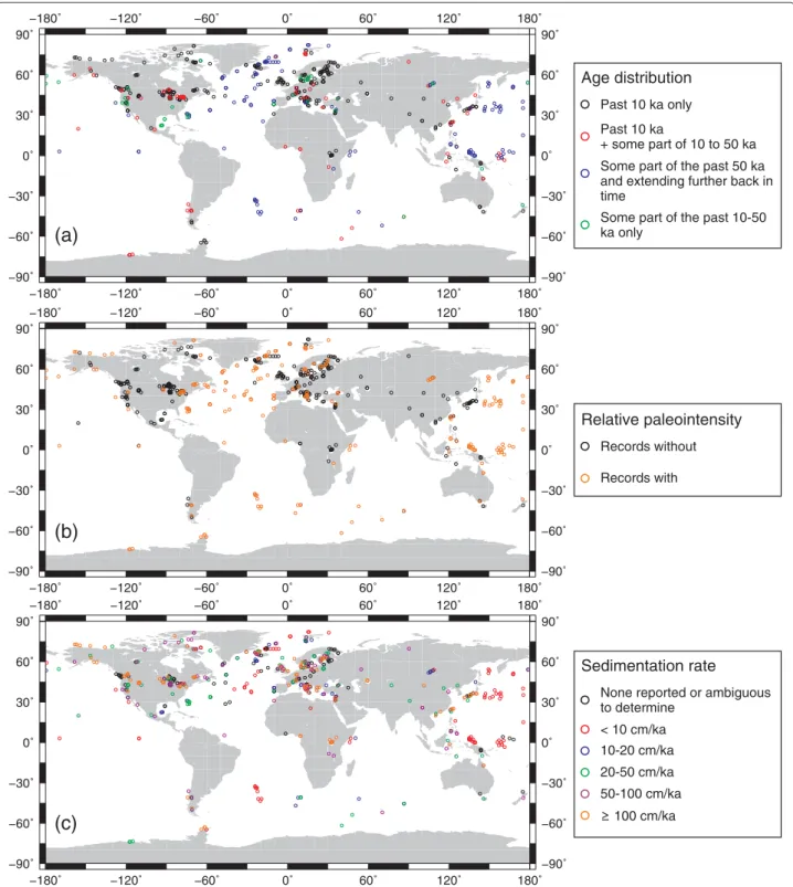
Although the data are globally distributed (Figure 3), over 85% of the cores are from the Northern Hemi-sphere. Figure 3 shows the geographic distribution of cores by the time period record by the sediments, whether relative paleointensity was measured and the division of cores based upon their average sedimentation rate. The earliest study is from 1970, and there has been an increasing number of studies per decade (compare 38 between 1970 and 1980 with 101 between 2000 and 2010; Figure 4). Most records do not span the full 50 ka, and a number of records cover only some part of the Holocene. Other records may be much longer, especially from marine environments, which may span from the present to several million years in the past (e.g., Hayashida et al. 1999; Valet and Meynadier 1993). Only the past 50 ka of records this length are currently available for download.
Data come from four sources:
1. an author directly,
2. a table in a publication or supplementary material, 3. another database (e.g., SECRV00, PANGAEA,
NOAA/NCDC, Janus or MagIC),
4. digitization of published graphic material.
The sources of the data are shown under the ‘Source ID’ entries in the results and metadata tables generated on querying the database. Data obtained from authors, publication tables and supplementary materials, or other databases are most reliable. Close communication with authors provides the most accurate reproduction of the data that appear in a publication. We have endeavored to provide the full data set as described in a publication.
Data from older publications are often not available in digital form; however, they can be digitized. These data are valuable for expanding the number of paleomagnetic measurements that can be used in global modeling of the geomagnetic field. However, caution must be exercised when using digitized data, as values cannot be precisely determined. Small uncertainties on digitized depth or age mean that although data can be from the same specimen or stratum, when parameters are digitized from different graphs (e.g., inclination and declination are shown on sep-arate axes), it is not possible to unequivocally link data to the same specimen/stratum. This is common when data are closely spaced in depth or time or if two discrete specimens were measured at the same depth. To be con-servative, each digitized datum is assigned a unique depth or age.
We have developed a digitization algorithm for pixel-based graphics using MATLAB. All digitized data in the database were obtained using this method. The algorithm considers rotation and distortion of the image. In some cases, axes are not precisely orthogonal, or the page is rotated. This is common for older articles where graph-ics have been scanned by us or a publisher. Automatic and manual data recognition are accommodated. Automatic data recognition is preferred where possible as it reduces the subjectivity associated with the manual selection of data. To estimate the deviation of manually defined points from their true coordinates, we digitized a graph of 100 randomly generated points with known coordinates at six levels of zoom. For these 600 points the mean deviation was 1.8%.
We encourage the scientific community to help in the population of the database by including data at the specimen/stratum level and averaged/smoothed level as Additional file 1 when publishing, following a table struc-ture similar to that of the GEOMAGIA50 .CSV output files (see the ‘Query results’ section).
Global models of the Holocene geomagnetic field
As described in Brown et al. (2015), coordinate-dependent predictions of inclination, declination, and intensity can be generated from five temporally con-tinuous global models of the Holocene geomagnetic field: CALS3k.4b, CALS10k.1b, ARCH3k.1, SED3k.1, and pfm9k.1a. A notable difference between the predic-tions produced through the sediment query (see the
(c)
(b)
(a)
Age distribution Past 10 ka only Past 10 ka + some part of 10 to 50 ka Some part of the past 50 ka and extending further back in timeSome part of the past 10-50 ka only Relative paleointensity Records without Records with Sedimentation rate < 10 cm/ka 10-20 cm/ka 20-50 cm/ka 50-100 cm/ka
None reported or ambiguous to determine
100 cm/ka
Figure 3 Global distribution of sediment cores documenting paleomagnetic field variations for some portion of the past 50 ka. (a) Cores by time
period, (b) cores with and without relative paleointensity records, and (c) cores by mean sedimentation rate. See the legends of the individual maps for further details.
‘Sediment query form’ section) and the archeo/volcanic query forms is that, with the exception of the ‘Coun-try/State/Region/Sea’ geographic constraint, the coordi-nates used are those from which the data were acquired, rather than the center of a geographical area. This allows
model predictions to be calculated down to the core level. Furthermore, we recommend users take care when com-paring location data with model predications generated using the ‘Country/State/Region/Sea’ geographic con-straint (Figure 5). For large geographic areas, latitude and
Figure 4 Number of sediment studies documenting paleomagnetic
field variations for some portion of the past 50 ka.
longitude can vary by tens of degrees; however, the model prediction will be generated for the geographic center of the area in question. A location’s coordinates can therefore be far from those used in the model query. For example, if Australia is selected from ‘Country/State/Region/Sea,’ the database will return results from Lake Keilambete, Victoria (Barton and McElhinny 1981), with a latitude of approximately 38°S; however, the geographic center of Australia is at 27°S. This stems in differences in inclination of approximately 10° between the data and model. This results purely from the geographic constraint selected and is not a limitation of the models.
Unlike for archeo/volcanic queries (Brown et al. 2015), model predictions are not plotted, as the variety of param-eters which could be plotted on different depth scales and age scales, and the large amount of data available for some locations, would greatly increase the time required to pro-cess each query. They are available for download only. See Brown et al. (2015) for descriptions of the column headers used in the model output files.
User interface: GEOMAGIA50 web page Sediment query form
The sediment query form (Figure 5) allows the user to search the database using data, age, and geographic con-straints. The link to the query form is found in the left navigation menu on the GEOMAGIA50 front page or by typing http://geomagia.gfz-potsdam.de/geomagiav3/ SDquery.php into the browser’s address bar. The form is divided into four sections:
1. Query, download and model options; 2. Advanced querying options;
3. Age constraints; 4. Geographic constraints.
These options are described in the following sections. A user’s guide to operating the query form is given in Additional file 1.
Query, download and model options
The top part of the query form (Figure 5) is divided into three sections: (i) paleomagnetic and rock magnetic data, (ii) age data, and (iii) model options. The data constraints in (i) and (ii) are directly related to four of the results tables described in the ‘Sediment database structure’ section, with the exception of the reconstructed paleomagnetic data results table. Therefore, (i) is subdivided into the following:
1. Individual (specimen/stratigraphic) data, 2. Processed (averaged/smoothed) data, and (ii) into the following:
1. Radiocarbon ages, 2. General ages.
Reconstructed paleomagnetic data are automatically queried when either ‘Individual (specimen/stratigraphic) data’ or ‘Processed (averaged/smoothed) data’ are selec-ted. ‘Model options,’ allows the user to query temporally continuous spherical harmonic models of the Holocene geomagnetic field (see the ‘Global models of the Holocene geomagnetic field’ section).
Age constraints
Data between 50 ka and the present can be queried, and the user can select all or part of this time interval (Figure 5). If no age constraints are selected, then data that are only on depth can also be retrieved (see Additional file 1: Section 1.1.2). This will be common for individual data from specific cores, as these data are often reported prior to application of an age-depth model. Age constraints are shown in years BP.
Geographic constraints
A great deal of flexibility in querying is provided within geographic constraints. The user can choose no geo-graphic constraints (useful for global searches of specific data types, see the‘Advanced querying options’ section) through to selecting data from a specific core (Figure 5 and Additional file 1: Section 1.1.3).
A significant portion of magnetic data from sediments from the past 50 ka come from marine cores. As marine cores are more commonly known by their location and core names (e.g., IODP, ODP, and MD site numbers), a dedicated field to search by core name has been included. Advanced querying options
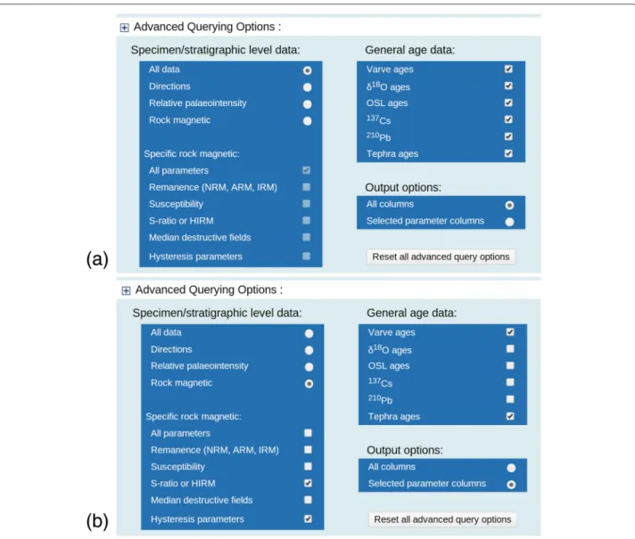
Advanced querying options enable more refined searches of the database (Figure 6). Options are available to mod-ify queries of individual paleomagnetic and rock magnetic data and general age data. No advanced querying options exist for processed paleomagnetic data or radiocarbon ages.
Figure 5 Sediment query form. Initial state of the sediment query form after the user has selected the ‘Sediment query form’ link from the left
navigation menu on the GEOMAGIA50 home page or entered http://geomagia.gfz-potsdam.de/geomagiav3/SDquery.php into a browser’s address bar.
Figure 6 Examples of the advanced query form with: (a) default options and (b) refined data querying and output options.
Individual data choices are split into three primary cate-gories: directional, RPI, and rock magnetic data (Figure 6). These splits are motivated by current research interests within paleomagnetism and rock magnetism. For exam-ple, RPI data alone can be used to improve our under-standing of the paleomagnetic power spectrum (Figure 1), and compilations of RPI data have been used to con-struct global and regional paleointensity stacks to aid in stratigraphic studies and to help in defining the global character of the geomagnetic field (see the ‘Introduc-tion’ section). Being able to filter out studies with no RPI data greatly increases the efficiency of these types of analyzes.
Environmental or climate studies may not require omagnetic data, with the exception of those using pale-omagnetic dating to infer the timing of environmental
or climate changes (e.g., Stott et al. 2002). Researchers may be interested in investigating certain parameters; therefore, searches for rock magnetic data can be further refined. More than one rock magnetic parameter can be queried at once (Figure 6b). The database returns entries that contain at least one of the rock magnetic parameters checked (‘or’ statements), e.g., if ‘Hysteresis parameters’ and ‘S-ratio or HIRM’ are selected, entries will be returned that contain either hysteresis or S-ratio/HIRM data. It does not limit the entries that are returned to those con-taining both hysteresis and S-ratio/HIRM data solely. This allows the user to view the complete entry for a specimen or horizon that contains the parameter(s) of interest. A range of data types are often used in combination to deter-mine magnetic grain size and deter-mineralogy. It is therefore advantageous to view all complementary data.
The choice of ‘General age data’ to be queried can also be refined (Figure 6). As with the rock magnetic param-eters, multiple general age constraints can be queried at once.
Advanced query options are useful for global compar-isons of data of the same type, especially data within the database that can be used to calculate ratios, e.g., rela-tive paleointensity data (NRM/ARM, NRM/IRM, NRM/k, VDM or VADM), S-ratio data, ARM/IRM, kARM/IRM,
and hysteresis data, e.g., Figure 7. Selecting no geographic and age constraints results in retrieval of many thousands of data (depending on the data type). These large data sets will allow comprehensive assessment of, e.g., rock magnetic biasing on relative paleointensity variations, fac-tors affecting the reliability of remanence acquisition, and the influence of depositional environments on magnetic parameters.
Query results
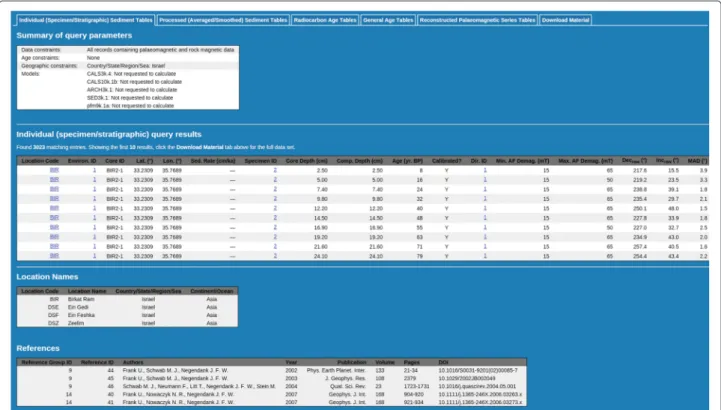
On executing the query (clicking ‘Perform Query’ at the bottom of the query form; Figure 5), a new tab will be launched in the browser. This contains six additional on-page tabs (Figure 8). Four of the tabs show the results of the four types of data queries described in the ‘Sediment database structure’ and ‘Query, download and model options’ sections. In addition, there is a tab showing
the results of any reconstructed paleomagnetic records (see the ‘Reconstructed paleomagnetic data results table’ section; we have included an example record from Lake Keilambete, Australia).
The final tab, ‘Download Material,’ contains hyper-links for up to five .CSV files and five .TXT files (Figure 9), depending on the data and models selected to query. The .CSV files contain the same fields and data as shown on the five on-page tabs. The only excep-tion is for null data. When no data exists for a cer-tain field in the online tables, a ‘-’ is shown. This is replaced in the .CSV files with −9999 for age data and 999 in all other cases. The .TXT files contain the out-put of the CALSxk and pfm9k.1a series of models (see the ‘Global models of the Holocene geomagnetic field’ section).
The column headers shown online and in the .CSV files are described in Additional file 1: Tables S1 to S6. Within the tables, the ordering of entries is governed sequentially, first by ‘Location Code’ (in alphabetical order), then ‘Core ID’ (in alphabetical order), ‘Core Depth (cm)’ or ‘Compos-ite Depth (cm)’ (depending on which is given; however, if both exist, data will be arranged by core depth), and finally ‘Age (yr. BP)’. Above the results tables, summaries of the query parameters chosen by the user are displayed (Figure 8). 1
Hcr/Hc
10 0.01 0.1 1Mrs/Ms
Orphan Knoll Lake Baikal Birkat Ram Central North Atlantic Ein Feshkha Grandfather Lake Lago di Mezzano Dunlop (2002) TM0 SD-MD Mixing Curves 0% SD 0% 0% 100% MD 100% 100% n = 3407 20% 40% 60% 80%Figure 7 Modified (Day et al. 1977) plot with single domain (SD) to multidomain (MD) mixing curves for magnetite (TM0) from Dunlop (2002).
Hysteresis parameters calculated for some example locations using ‘Advanced querying options’ with no geographic or age constraints. Orphan Knoll (IODP Sites U1302-U1303; Channell et al. 2012), Lake Baikal (Peck et al. 1994), Birkat Ram (Israel; Frank et al. 2003), Central North Atlantic (IODP Site U1308; Channell et al. 2008), Ein Feshka (Dead Sea; Frank et al. 2007), Grandfather Lake (Alaska; Geiss and Banerjee 2003), Irminger Basin (ODP Site 919; Channell 2006), and Lago di Mezzano (Italy; Frank 1999). n is the number of data.
Figure 8 The appearance of the results web page showing the six on-page tabs. The first few output columns of the ‘Individual Specimen/
Stratigraphic Level Sediment Tables’ tab are shown for an example query from Israel, along with two examples of relational tables (‘Location Names’ and ‘References’) accompanying this query. The underlined entries are hyperlinks.
Each table contains a number of fields that list the IDs (see the ‘Metadata tables and identification num-bers’ section), e.g., the references (Figure 8). Each ID is a hyperlink. On clicking a hyperlink, the page scrolls down to a relational table describing the ID (Figure 8). The relational tables (see the ‘Metadata tables and
identifica-tion numbers’ secidentifica-tion) are found beneath the results table (Figure 8).
If no constraints are selected, then the user is redirected to the web page ‘Complete sediment data sets.’ This page contains hyperlinks to pre-prepared .CSV files with the complete data from the five results tables. At the time of
Figure 9 The appearance of the ‘Download Material’ tab. The left column lists all possible categories of data that can be downloaded. The right
column gives the user the option to download data files via hyperlinks, depending on whether the query returned any results for a particular category of data.
writing, the number of data entries exceeds 30,000, with multiple data available for each entry. Such a large amount of data takes a prohibitively long time to print to the screen. To further reduce the execution time of the query, we limit the output printed to the screen to the first 10 entries that match the constraints specified by the user (all data matching the specified constraints are written to the file).
Conclusions
The GEOMAGIA50 database for sediments is an expan-sion of the GEOMAGIA50 database, which previously housed only magnetic data from archeological and vol-canic materials (Brown et al. 2015; Donadini et al. 2006; Korhonen et al. 2008). The database accommodates paleo-magnetic, rock paleo-magnetic, radiocarbon, and other age data obtained from marine and lake sediments deposited over the past 50 ka. Data from sediments help constrain inter-pretations of past changes in the geomagnetic field, the environment, and climate. We document in detail radio-carbon age data, as well as210Pb,137Cs,δ18O, varve, and tephra age information. For all data types, uncertainties are reported where possible.
The database can be accessed through a web query form, which can be found at http://geomagia.gfz-potsdam. de/geomagiav3/SDquery.php and is mirrored at http:// geomagia.ucsd.edu/. The interface has been designed to allow rapid selection of data by age, geographic, and data type constraints. More advanced queries based upon spe-cific paleomagnetic, rock magnetic, and chronological types are accommodated. This enables global compar-isons of specific data types. The results of queries can be viewed online and downloaded as .CSV files. In addition, users can generate Holocene geomagnetic field model predictions from the CALSxk and pfm9k.1a series of mod-els (e.g., Korte and Constable 2011; Nilsson et al. 2014) for the coordinates used for the data search. These data can be downloaded as .TXT files.
Owing to the large amount of data available from sedi-ments, approximately 300 studies report results from over 700 sediment cores, the uploading of material is ongo-ing. In addition, new data are frequently obtained from sediments, and the database will be updated as these are published.
Availability and requirements Project name:GEOMAGIA50
Project home page:http://geomagia.gfz-potsdam.de/ Operating system(s):Platform and browser independent Programming language:PHP, SQL, HTML, JavaScript, Python, Fortran
Other requirements:Google Earth plug-in License:none
Any restrictions to use by non-academics:none
Additional file
Additional file 1: An additional file contains a user’s guide to the sediment database. This guide is the second of a pair describing the
function of the GEOMAGIA50.v3 database.
Competing interests
The authors declare that they have no competing interests.
Authors’ contributions
MCB participated in the design of the database, its implementation and web design, data acquisition, and drafted the manuscript. FD and KK participated in the design of the database and implemented its underlying operational principles. AN, CGC, MK, SP, and UF participated in aspects of the database design and/or data acquisition. CGC conducted the dipole power spectrum analysis. CGC and MK contributed to the drafting of the manuscript. MS designed the digitization software. All authors read and approved the final manuscript.
Acknowledgements
We kindly thank those who provided data in a digital form. Lisa Tauxe is thanked for providing her SEDPI06 data compilation. MCB, MK, and MS were supported by Deutsche Forschungsgemeinshcaft (DFG) SPP PlanetMag 1488 projects (KO2870/4-1, BR4697/1 and WA2605/2). FD acknowledges the support of the Swiss National Science Foundation (project numbers 130147 and 144102). AN was funded by the Natural Environment Research Council (NE/I013873/1) and the Swedish Research Council (Dnr 2014-4125). SP was funded by US National Science Foundation NSF grant EAR 1246826. CGC gratefully acknowledges support from the Alexander von Humboldt Foundation and US National Science Foundation Grant NSF EAR 12225364. Gesa Petersen is thanked for uploading a substantial amount of data to the database. Two anonymous reviewers are thanked for their comments.
Author details
1GFZ German Research Centre for Geosciences, Telegrafenberg, 14473 Potsdam, Germany.2Department of Earth Sciences, University of Fribourg, Chemin du Musée 6, 1700 Fribourg, Switzerland.3Geomagnetism Laboratory, Department of Earth, Ocean and Ecological Sciences, University of Liverpool, L69 7ZE Liverpool, UK.4Current address: Department of Geology, Quaternary Sciences, Lund University, Sölvegatan 12, 223-62 Lund, Sweden.5Institute of Geophysics and Planetary Physics, Scripps Institution of Oceanography, University of California, La Jolla, San Diego, CA 92092-0225, USA.6Geological Survey of Finland, P.O. Box 96 (Betonimiehenkuja 4), FI-02151 Espoo, Finland. 7Institute of Earth and Environmental Science, University of Potsdam, 14476 Potsdam, Germany.8Current address: Faculty of Civil Engineering and Geosciences, Delft University of Technology, 2628 CN Delft, Netherlands. Received: 4 February 2015 Accepted: 17 April 2015
References
Amit H, Leonhardt R, Wicht J (2010) Polarity reversals from paleomagnetic observations and numerical dynamo simulations. Space Sci Rev 155:293–335. doi:10.1007/s11214-010-9695-2
Barton CE, McElhinny MW (1981) A 10000 yr geomagnetic secular variation record from three Australian maars. Geophys J R astr Soc 67:465–485. doi:10.1111/j.1365-246X.1981.tb02761.x
Biggin AJ, Strik GHMA, Langereis CG (2009) The intensity of the geomagnetic field in the late-Archaean: new measurements and an analysis of the updated IAGA palaeointensity database. Earth Planets Space 61:9–22. doi:10.1186/BF03352881
Biggin AJ, McCormack A, Roberts A (2010) Paleointensity database updated and upgraded. EOS Trans Am Geophys Union 91(2):15.
doi:10.1029/2010EO020003
Blaauw M, Christen JA (2011) Flexible paleoclimate age-depth models using an autoregressive gamma process. Bayesian Analysis 6:457–474. doi:10.1214/11-BA618
Bloemendal J, deMenocal P (1989) Evidence for a change in the periodicity of tropical climate cycles at 2.4 Myr from whole-core magnetic susceptibility measurements. Nature 342:897–900. doi:10.1038/342897a0
Bloemendal J, King JW, Hall FR, Doh S-J (1992) Rock magnetism of Late Neogene and Pleistocene deep-sea sediments: relationship to sediment source, diagenetic processes and sediment lithology. J Geophys Res 97(B4):4361–4375. doi:10.1029/91JB03068
Bowler JM, Hamada T (1971) Late Quaternary stratigraphy and radiocarbon chronology of water level fluctuations in Lake Keilambete, Victoria. Nature 232:330–332. doi:10.1038/232330a0
Brown MC, Jicha BR, Singer BS, Shaw J (2013) Snapshot of the
Matuyama-Brunhes reversal process recorded in40Ar/39Ar-dated lavas from Guadeloupe, West Indies. Geochem Geophys Geosyst 14:4341–4350. doi:10.1002/ggge.20263
Brown MC, Donadini F, Korte M, Nilsson A, Korhonen K, Lodge A, Lengyel SN, Constable CG (2015) GEOMAGIA50.v3: 1. general structure and modifications to the archeological and volcanic database. Earth Planets Space. doi:10.1186/s40623-015-0232-0
Carter-Stiglitz B, Valet J-P, LeGoff M (2006) Constraints on the acquisition of remanent magnetization in fine-grained sediments imposed by redeposition experiments. Earth Planet Sci Lett 245:427–437. doi:10.1016/j.epsl.2006.03.002
Channell JET (2006) Late Brunhes polarity excursions (Mono Lake, Laschamp, Iceland Basin and Pringle Falls) recorded at ODP Site 919 (Irminger Basin). Earth Planet Sci Lett 244:378–393. doi:10.1016/j.epsl.2006.01.021 Channell JET, Hodell DA, Lehman B (1997) Relative geomagnetic paleointensity
andδ18O at ODP Site 983 (Gardar Drift, North Atlantic) since 350 ka. Earth Planet Sci Lett 153:103–118. doi:10.1016/S0012-821X(97)00164-7 Channell JET, Stoner JS, Hodell DA, Charles CD (2000) Geomagnetic
paleointensity for the last 100 kyr from the sub-antarctic South Atlantic: a tool for inter-hemispheric correlation. Earth Planet Sci Lett 175:145–160. doi:10.1016/S0012-821X(99)00285-X
Channell JET, Hodell DA, Xuan C, Mazaud A, Stoner JS (2008) Age calibrated relative paleointensity for the last 1.5 Myr at IODP Site U1308 (North Atlantic). Earth Planet Sci Lett 274:59–71. doi:10.1016/j.epsl.2008.07.005 Channell JET, Xuan C, Hodell DA (2009) Stacking paleointensity and oxygen
isotope data for the last 1.5 Myr (PISO-1500). Earth Planet Sci Lett 283:14–23. doi:10.1016/j.epsl.2009.03.012
Channell JET, Hodell DA, Curtis JH (2012) ODP Site 1063 (Bermuda Rise) revisited: Oxygen isotopes, excursions and paleointensity in the Brunhes chron. Geochem Geophys Geosyst 13:Q02001. doi:10.1029/2011GC003897
Clark RM (1979) Calibration, cross-validation and carbon-14. I. J R Stat Soc A 142:47–62. doi:10.2307/2344653
Coe RS, Glen JMG (2004) The complexity of reversals. In: Channell JET, Kent DV, Lowrie W, Meert JG (eds). Timescales of the Paleomagnetic Field. American Geophysical Union, Washington, D.C. pp 221–232. doi:10.1029/145GM16 Coe RS, Grommé S, Mankinen EA (1978) Geomagnetic paleointensities from
radiocarbon-dated lava flows on Hawaii and the question of the Pacific nondiple low. J Geophys Res 83(B4):1740–1756.
doi:10.1029/JB083iB04p01740
Constable C, Johnson C (2005) A paleomagnetic power spectrum. Phys Earth Planet Inter 153:61–73. doi:10.1016/j.pepi.2005.03.015
Constable C, Korte M (2006) Is Earth’s magnetic field reversing? Earth Planet Sci Lett 246:1–16. doi:10.1016/j.epsl.2006.03.038
Constable C, Koppers A, Tauxe L, Minnett RC (2006) Five dimensions of MagIC. EOS Trans Am Geophys Union 87(52):13–1172
Davies CJ, Constable CG (2014) Insights from geodynamo simulations into long-term geomagnetic field behaviour. Earth Planet Sci Lett 404:238–249. doi:10.1016/j.epsl.2014.07.042
Day R, Fuller M, Schmidt VA (1977) Hysteresis properties of titanomagnetites: grain size and compisitional dependence. Phys Earth Planet Inter 13:260–267. doi:10.1016/0031-9201(77)90108-X
De Deckker P (1982) Holocene ostracods, other invertebrates and fish remains from cores of four maar lakes in southeastern Australia. Proc R Soc Victoria 94:183–219
Denham CR (1981) Numerical correlation of recent paleomagnetic records in two Lake Tahoe cores. Earth Planet Sci Lett 54:48–52.
doi:10.1016/0012-821X(81)90067-4
Diepenbroek M, Grobe H, Reinke M, Schindler U, Schlitzer R, Sieger R, Wefer G (2002) PANGAEA - an information system for environmental sciences. Comput Geosci 28:1201–1210. doi:10.1016/S0098-3004(02)00039-0 Dodson JR (1974) Vegetation and climatic history near Lake Keilambete,
Western Victoria. Australian J Botany 22:709–717. doi:10.1071/BT9740709
Donadini F, Korhonen K, Riisager P, Pesonen LJ (2006) Database for Holocene geomagnetic intensity information. EOS Trans Am Geophys Union 87(14):137–143. doi:10.1029/2006EO140002
Donadini F, Korte M, Constable CG (2009) Geomagnetic field for 0-3 ka: 1. New data sets for global modeling. Geochem Geophys Geosyst 10:Q06007. doi:10.1029/2008GC002295
Driscoll P, Olson P (2009) Polarity reversals in geodynamo models with core evolution. Earth Planet Sci Lett 282:24–33. doi:10.1016/j.epsl.2009.02.017 Dunlop DJ (2002) Theory and application of the Day plot (Mrs/Msversus
Hcr/Hc) 1. Theoretical curves and tests using titanomagnetite data. J Geophys Res 107(B3):2056. doi:10.1029/2001JB000486
Fisher RA (1953) Dispersion on a sphere. Proc R Soc Lond A 217:295–305. doi:10.1098/rspa.1953.0064
Frank U (1999) Rekonstruktion von Säkularvariationen des Erdmagnetfeldes der letzten 100.000 Jahre - Untersuchungen an Sedimenten aus dem Lago di Mezzano und dem Lago Grande di Monticchio, Italien. PhD thesis, Univ. of Potsdam
Frank U, Nowaczyk NR, Negendank JFW, Melles M (2002) A paleomagnetic record from Lake Lama, northern Central Siberia. Phys Earth Planet Inter 133:3–20. doi:10.1016/S0031-9201(02)00088-2
Frank U, Schwab MJ, Negendank JFW (2003) Results of rock magnetic investigations and relative paleointensity determinations on lacustrine sediments from Birkat Ram, Golan Heights (Israel). J Geophys Res 108(B8):2379. doi:10.1029/2002JB002049
Frank U, Nowaczyk NR, Negendank JFW (2007) Rock magnetism of greigite bearing sediments from the Dead Sea, Israel. Geophys J Int 168:921–934. doi:10.1111/j.1365-246X.2006.03273.x
Frank U, Nowaczyk N. R, Minyuk P, Vogel H, Rosén P, Melles M (2013) A 350 ka record of climate change from Lake El’gygytgyn, Far East Russian Arctic: refining the pattern of climate modes by means of cluster analysis. Clim Past 9:1559–1569. doi:10.5194/cp-9-1559-2013
Geiss CE, Banerjee SK (2003) A Holocene-Late Pleistocene geomagnetic inclination record from Grandfather Lake, SW Alaska. Geophys J Int 153:497–507. doi:10.1046/j.1365-246X.2003.01921.x
Granot R, Dyment J, Gallet Y (2012) Geomagnetic field variability during the Cretaceous Normal Superchron. Nature Geosci 5:220–223.
doi:10.1038/ngeo1404
Guyodo Y, Valet J-P (1999a) Integration of volcanic and sedimentary records of paleointensity: constraints imposed by irregular eruption rates. Geophys Res Lett 26:3669–3672. doi:10.1029/1999GL008422
Guyodo Y, Valet J-P (1999b) Global changes in intensity of the Earth’s magnetic field during the past 800 kyr. Nature 399:249–252. doi:10.1038/20420 Guyodo Y, Gaillot P, Channell JET (2000) Wavelet analysis of relative
geomagnetic paleointensity at ODP site 983. Earth Planet Sci Lett 184:109–123. doi:10.1016/S0012-821X(00)00313-7
Haltia-Hovia E, Nowaczyk N, Saarinen T (2011) Environmental influence on relative palaeointensity estimates from Holocene varved lake sediments in Finland. Phys Earth Planet Inter 185:20–28. doi:10.1016/j.pepi.2010.12.002 Hayashida A, Verosub KL, Heider F, Leonahardt R (1999) Magnetostratigraphy and relative palaeointensity of late Neogene sediments at ODP Leg 167 Site 1010 off Baja California. Geophys J Int 139:829–840.
doi:10.1046/j.1365-246x.1999.00979.x
Heslop D, Roberts AP, Hawkins R (2014) A statistical simulation of magnetic particle alignment in sediments. Geophys J Int 197:828–837. doi:10.1093/gji/ggu038
Jackson A, Jonkers ART, Walker MR (2000) Four centuries of geomagnetic secular variation from historical records. Phil Trans R Soc Lond A 358:957–990. doi:10.1098/rsta.2000.0569
Jackson M, Bowles J, Lascu I, Solheid P (2010) Deconvolution of u channel magnetometer data: experimental study of accuracy, resolution and stability of different inversion methods. Geochem Geophys Geosyst 11:Q07Y10. doi:10.1029/2009GC002991
Jarboe NA, Koppers AA, Tauxe L, Minnett R, Constable CG (2012) The online MagIC Database: data archiving, compilation, and visualization for the geomagnetic, paleomagnetic and rock magnetic communities. Am Geophys Union Fall Meeting Abstracts 1:1063
Johansson A, Lehnert K, Hsu L (2012) Status report on the SedDB Sediment Geochemistry Database: March, 2012. GeoPRISMS Newslett 28:21 Katari K, Bloxham J (2001) Effects of sediment aggregate size on DRM intensity:
a new theory. Earth Planet Sci Lett 186:113–122. doi:10.1016/S0012-821X(00)00386-1