HAL Id: hal-02050477
https://hal-montpellier-supagro.archives-ouvertes.fr/hal-02050477
Submitted on 27 Feb 2019HAL is a multi-disciplinary open access archive for the deposit and dissemination of sci-entific research documents, whether they are pub-lished or not. The documents may come from teaching and research institutions in France or abroad, or from public or private research centers.
L’archive ouverte pluridisciplinaire HAL, est destinée au dépôt et à la diffusion de documents scientifiques de niveau recherche, publiés ou non, émanant des établissements d’enseignement et de recherche français ou étrangers, des laboratoires publics ou privés.
Towards a holistic approach for multi-objective
optimization of food processes: a critical review
Martial Madoumier, Gilles Trystram, Patrick Sébastian, Antoine Collignan
To cite this version:
Martial Madoumier, Gilles Trystram, Patrick Sébastian, Antoine Collignan. Towards a holistic ap-proach for multi-objective optimization of food processes: a critical review. Trends in Food Science and Technology, Elsevier, 2019, 86, pp.1-15. �10.1016/j.tifs.2019.02.002�. �hal-02050477�
Towards a holistic approach for multi-objective optimization
1
of food processes: a critical review
2
Martial Madoumier a, Gilles Trystram b, Patrick Sébastian c, Antoine Collignan a
3
a QualiSud, Montpellier SupAgro, CIRAD, Univ d'Avignon, Univ Montpellier, Univ de La Réunion,
4
Montpellier, France
5
b Université Paris-Saclay, Agroparistech, Inra, UMR 1145, F-75005 Paris, France
6
c Université de Bordeaux, I2M, UMR CNRS 5295, Esplanade des Arts et Métiers, 33405 Talence
7
cedex, France
8
Abstract
9While Multi-objective Optimization (MOO) has provided many methods and tools for 10
solving design problems, food processes have benefitted little from them. MOO 11
encompasses the identification of performance indicators, process modelling, preference 12
integration, trade-off assessment, and finding the best trade-offs. In this review, the use 13
of these five elements in the design of food processes through MOO is analysed. A 14
number of studies dealing with food processes MOO have been identified. Even though 15
these studies improve the design process, they often approach MOO in a simplified and 16
insufficiently rationalized way. Based on this review, several research issues are 17
identified, related to the improvement of the different models and methods, and to the 18
development of more holistic MOO methods for food processes. 19
Key words
20Multi-objective optimization; food process design; multi-criteria decision aids 21
1. Introduction
22In food process engineering, most design problems are aimed at several objectives, 23
which can often be contradictory. Thus, maximizing food product quality (texture, 24
nutrients concentration, flavour…) is often in conflict with process performance 25
objectives, such as minimizing energy consumption, maximizing profit, or ensuring 26
safety in the case of heat treatments. For the last two decades, solving multi-objective 27
design problems has been a major concern as sustainable development practices also 28
need to be integrated in the design process. Many kinds of objectives can be defined by 29
the decision-maker, all with potential antagonistic effects, e.g. maximizing one has the 30
effect of minimizing one or several others. 31
32
To solve multi-objective design problems, different kinds of methods have been 33
developed, with the earliest being gradient-based methods and experiments-based 34
methods. Gradient-based methods, such as the method of Lagrange multipliers, are 35
based on the resolution of differentiable equation systems, and although they yield fast 36
computation times, they converge toward local optima only, which may not be global 37
optima. Experiments-based methods, and more specifically Response Surface 38
Methodology, were and remain a common optimization approach in the food processing 39
industry (Banga et al., 2008). Since then, new optimization methods for multi-objective 40
problems have been developed, which are able to efficiently identify global optima. They 41
have been grouped under the term “multi-objective optimization (MOO) methods”. 42
43
MOO is a general methodology aimed at identifying the best trade-off(s) between 44
several conflicting objectives. Numerous applications in engineering can be found, from 45
the design of a single mechanical part (Collignan et al., 2012) to the optimization of a 46
worldwide supply chain (Wang et al., 2011). MOO consists in a) a multi-objective 47
processing method, to transform the original multi-objective problem into a solvable 48
problem, and b) an optimization algorithm, to search for trade-off solutions to the 49
multi-objective problem (Collette and Siarry, 2013). 50
51
A multi-objective processing method requires the following elements, in the food 52
processes framework: 53
1) Optimization objectives and associated indicators. The decision maker defines 54
objectives, i.e. changes that the decision-maker(s) wish(es) to cause in the
55
process (profit increase, productivity increase, environmental impact decrease…), 56
and these changes are quantified or described by suitable performance 57
indicators (margin, yield, carbon dioxide emissions…) (Church and Rogers,
58
2006). Indicators are also called by the term “criteria”, which can itself be used as 59
an equivalent to “objectives” (Craheix et al., 2015). In this work, the terminologies 60
“objectives” and “indicators” will be used. 61
2) A predictive food process model: the effect of different values of the design 62
variables (input variables, i.e. operating conditions, equipment size, process 63
structure...) on the indicators is predicted by a process model. Thus, the different 64
design solutions available can be evaluated. The predictive model should provide 65
a satisfying level of prediction accuracy, while optimizing efficiently for reasonable 66
computation times. 67
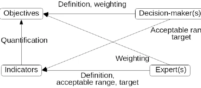
3) A preference model, where the decision-maker preferences and expert 68
knowledge are integrated. Preferences may be specified at two different levels
69
(figure 1): i) objectives may be weighted according to their relative significance for 70
the decision-maker and/or qualified experts; ii) desirability functions may be used 71
to integrate satisfaction levels of experts according to indicator values. The 72
decision-maker may have sufficient knowledge to specify preferences at both 73
levels. However, it is considered in this work that the experts have more 74
qualifications to specify preferences on indicator values, based on a good 75
scientific and/or technical knowledge of the process and the installation context. 76
77
Figure 1: Relationships between objectives, indicators, and preference integration
78
4) A selection method to choose the “best trade-off” by sorting, ranking or scoring 79
the design solutions available. The selection method generally consists in 80
aggregating preferences and indicators to build an objective function for 81
optimization, but may also in consist in different approaches. 82
83
Regarding the optimization algorithm, it integrates these four elements to search for 84
trade-offs among possible design solutions. 85
86
Numerous methods and algorithms can be used to build a multi-objective processing 87
method to be combined with an optimization algorithm. Detailed taxonomies and 88
information on these methods can be found in reference books such as (Chen and 89
Hwang, 1992; Collette and Siarry, 2013; Ehrgott, 2005; Miettinen, 1998). It is also 90
noteworthy that predictive food process models and preferences models are used in 91
single-objective (mono-objective) optimization, in order to obtain a single performance 92
indicator. These elements are not specific to MOO, and a detailed comparison of single- 93
and multi-objective optimization can be found in Rangaiah et al. (2015). 94
95
In this context, the application of MOO to food processing was studied, that is the 96
transformation of biological raw materials by one or several unit operations to produce 97
edible food products. The investigation field of this review was restricted to MOO for 98
food process design, which excludes: 99
process control (or closed loop optimal control, as defined in Banga et al. (2008) 100
– see for example Trelea et al. (1997)); 101
product formulation (or mixture design - see for example Chen et al. (Chen et al., 102
2004)); 103
model parameter optimization. 104
The design problems included were: 105
selection of fixed or variable operating conditions (i.e. open loop optimal control – 106
Banga et al. (2008)); 107
equipment sizing; 108
number and structure of unit operations in the process. 109
A number of articles have been reviewed to discuss the methods used by the authors to 110
perform MOO. From these studies it was established that despite the advanced 111
development of MOO as a generic design methodology, the tools and methods of MOO 112
have not yet fully reached the area of food process design: 113
MOO is infrequent in the design of food processes compared to chemical 114
processes: around 40 articles on MOO application in food processing had been 115
published in scientific journals before 2009 (Abakarov et al., 2009), whereas 116
around 360 papers regarding MOO in chemical engineering applications had 117
been published until mid-2012 (Rangaiah and Bonilla-Petriciolet, 2013). Several 118
authors (Banga et al., 2003; Trystram, 2012) have identified two major 119
hindrances: i) physical properties, and consequently quality parameters of food 120
materials, are difficult to predict because of the complexity of food materials; ii) 121
many food process models are unsuitable for optimization purposes, since they 122
have been developed to understand the behaviour of food materials as biological 123
reactors (with reaction kinetics and transfers), rather than predict its behaviour as 124
a function of process control variables and size. 125
Most studies focus on the optimization of operating conditions for design or 126
process control; many of them concern heat treatment processes. In contrast only 127
a few MOO studies concentrate on the integrated design of food processes, 128
where both unit operations structure and equipment sizing are optimized (see for 129
example Nishitani and Kunugita (1979)). 130
Most MOO design studies published are limited to the production of the Pareto 131
front, i.e. the set of trade-off solutions for the process design (Kiranoudis and 132
Markatos, 2000; Kopsidas, 1995; Nishitani and Kunugita, 1979, 1983; Stefanis et 133
al., 1997; Yuen et al., 2000 …). Multi-criteria decision making (MCDM) methods, 134
which help to select the best trade-off amongst Pareto-efficient solutions, are 135
seldom applied in these studies. MCDM methods can help include the 136
preferences of the decision-maker in the design process, and rank the possible 137
solutions to identify one (or a small set of) “best” trade-off(s) for process design. 138
Very few design approaches are systemic: most optimization objectives are 139
evaluated with “raw” indicators of process performance (nutrient retention, energy 140
consumption, processing time…) and do not involve the interactions of the 141
process with its environment (environmental impact based on LCA, overall 142
economic profit, nutritional interest…). 143
Thus, the potential for developing more advanced MOO methods and associated tools 144
for the design of food processes is high: most studies only partially use the constituent 145
elements of MOO, while a variety of methods and tools are available to perform MOO. 146
Hence it seemed relevant to study and review these methods and tools along with their 147
use for food process design. 148
In this paper, a critical review of multi-objective optimization methods which have
149
been used in food process design studies is developed. The main purpose is to
150
demonstrate how design methods engineering can solve design problems in food
151
processing, which however requires a choice among existing MOO methods.
152
The different sections of this review match the aforementioned elements which 153
constitute a MOO method: 154
Section 2 is a critical analysis of indicators which describe design objectives; 155
Section 3 briefly reviews process models used for MOO of food processes; 156
Section 4 deals with the integration of preferences in decision-making; 157
Section 5 handles the methods used in the literature to select the best 158
solutions;
159
Section 6 explores optimization algorithms for MOO from the perspective of 160
methods engineering; 161
Section 7 describes some holistic MOO methods, which include all elements for 162
MOO (process indicators and model, preference model, ranking method, 163
optimization algorithm) and discusses research issues. 164
2. Design indicators
1652.1. Raw and integrative indicators
166
The indicators required for optimization are produced by a set of more or less complex 167
models, based on knowledge of the process. The indicators are mostly quantitative, but 168
may possibly be qualitative (one product more appreciated than another, soft or hard 169
texture, sanitary risk present or absent, etc.); the latter case is not considered in this 170
work. A quantitative indicator may be an integer variable, but is more generally a real 171
variable in the field of food processing. Process sizing parameters, such as a number of 172
effects of an evaporator or number of cleaning cycles, may be represented by an 173
variable integer, which is common in the field of chemical processing (see for example 174
Morandin et al. (2011) and Rangaiah and Bonilla-Petriciolet (2013)). Quantitative 175
indicators can be constructed simply using the physical variables (or chemical, 176
biochemical, biological variables) of the process, or be generated by an economic model 177
or environmental impact model, making it possible to quantify global objectives 178
(especially sustainability). In this work, the indicators are categorized in two families: 179
Raw indicators, i.e. variables of physical, chemical, biochemical or even biological 180
origin, calculated using the process model, such as the product treatment 181
temperature, its sensorial qualities (texture, colour…), steam consumption, 182
retention rate of a compound of interest, etc. 183
Integrative indicators, which combine raw indicators referring to different (but 184
linked) phenomena into a unique variable, according to scientific and/or technical 185
or statistical principles, or even rule-like principles. They are constructed from 186
economic, environmental, social, or even product quality models. They 187
correspond to the definition of the composite indicators given by Von Shirdning 188
(2002). 189
190
In the case of raw indicators, interpretation i.e. the relationship between indicators and 191
objectives, is left to the decision-maker, which assumes a degree of expertise in the 192
process under study. A decision-maker not specializing in the process will be less 193
capable of analysing the solutions proposed, since the raw indicators may not be explicit 194
in terms of the objectives sought. Thus, the exergy proposed by Nishitani and Kunugita 195
(1983) requires an ability to understand this concept in terms of environmental impact; 196
the “head kernel” yield for optimizing rice drying by Olmos et al. (2002) cannot quantify 197
the economic implications of this indicator. Similarly, selecting a raw indicator could 198
partly conceal, or even bias, the information required for evaluating the objectives. Thus 199
Stefanis et al. (1997) opted to characterize the environmental impact in wastewater by 200
BOD (Biological Oxygen Demand), which represents a highly partial view of the 201
environmental impact that a process may have. In Nishitani and Kunugita (1979), the 202
exchange surface contributes only partially to the cost of the evaporator, and so appears 203
to be an incomplete indicator in terms of the defined economic objective. 204
Conversely, raw indicators can be tailored to specific contexts, where the process 205
objectives can be expressed directly by physical variables derived from the process 206
model: in Yuen et al. (2000), the objective is to remove alcohol from beer while 207
minimizing loss of chemicals associated with taste, which is explicitly expressed by an 208
“alcohol removal” indicator and an “extract removal” indicator. In particular in the case of 209
explicitly known product quality objectives, they can be expressed by selecting certain 210
nutritional compounds, such as in Tarafdar et al. (2017), where the indicators are 211
contents of nutritional compounds of interest. 212
213
On ther other hand, integrative indicators can link the process physical variables to 214
variables of interest/which are meaningful for the decision-maker: a return on investment 215
time for example will be easier to interpret for an investor than an investment cost and 216
an operating cost taken separately. Sebastian et al. (2010) defined a total cost of 217
ownership, bringing together the operating cost (electricity and fluids consumption) and 218
an investment cost (purchasing and manufacturing costs), which can be used to quantify 219
what the equipment costs over a planned service life of twenty years. 220
However, due to the construction of the associated functions, integrative indicators entail 221
a risk of bias in the interpretation. Firstly, the models used may be subject to debate; in 222
the case of impact scores based on Life Cycle Analysis (LCA) for example, modelling of 223
the environmental impacts varies according to the impact calculation methodologies, and 224
there is not always an established consensus on these models (Hauschild et al., 2008). 225
Then, the weighting of different kinds of indicators (greenhouse effect and 226
eutrophication, texture and colour…) for the purpose of aggregating them in an 227
integrative indicator may also entail a bias. Finally, constructing integrative indicators 228
assumes use of data which is sometimes uncertain; thus it is not always possible, at the 229
scale of a process situated in a larger system (e.g. factory), to predict its profitability or 230
maintenance cost. 231
232
The indicators encountered in the various articles studied in this work are rarely 233
integrative indicators. While aggregating raw indicators can produce an indicator which 234
is meaningful for the decision-maker, the way in which they are grouped induces a risk 235
of information loss. Thus, raw indicators of major significance in design choices may find 236
themselves concealed by the integrative indicator, as in the case of the SAIN-LIM 237
indicator which conceals the effect of certain nutrients on the overall score (Achir et al., 238
2010). So the development of relevant indicators means finding a balance between an 239
excessive number of raw indicators, which is difficult to interpret and discuss, and an 240
integrative indicator, which would cause major information loss through aggregation. 241
2.2. Relevance of indicators
242
Besides the advantages and shortcomings of raw and integrative indicators, the 243
question of choice of indicators is an issue of interest, firstly in terms of the meaning 244
given to the indicators. There are numerous approaches for constructing more or less 245
integrative indicators which are meaningful for the decision-maker in view of their 246
objectives. An overview of some of these approaches is proposed here, via the four 247
dimensions of sustainability of food engineering processes: economic sustainability and 248
product quality, which are the most frequently encountered dimensions, plus 249
environmental and social sustainability. 250
251
Economic evaluation of processes makes it possible to establish the cost that they 252
represent, and/or their profitability in the shorter or longer term. In the context of 253
optimization, it must be possible to predict their operating cost and the investment they 254
represent; there are correlations for predicting investment as a function of sizing 255
choices, the best known of which is from Guthrie (1969). Benchmark works provide 256
values for the parameters of this correlation (Maroulis and Saravacos, 2007; Turton et 257
al., 2008). Based on the economic and financial information on the process and the 258
company, it becomes possible to construct integrative economic indicators, the best 259
known of which are the internal profitability rate, return on investment time, discounted 260
income, net present value and net cumulative cash flow (Chauvel et al., 2001; Turton et 261
al., 2008). Other approaches are being developed, such as thermo-economics, which 262
associates a cost with exergy (a measure of energy quality to determine energy 263
degradation in the system), to evaluate economic feasibility and profitability (Rosen, 264
2008). In keeping with the “life cycle” approach, Life Cycle Costing (LCC), where the 265
financial, environmental and social costs are factored into the life cycle as a whole 266
(Norris, 2001), is another approach under development. Like thermo-economics, it still 267
requires construction of databases large enough for the economic indicators proposed to 268
evaluate the food engineering processes. 269
270
Food quality needs to be described through a holistic perspective which covers all 271
consumer requirements. Among several possible approaches, an attempt was made by 272
Windhab (2009) to provide such holistic perspective, known by the acronym PAN: 273
Preference (organoleptic and usage properties), Acceptance (religious, cultural, 274
GMO…), Need (health, nutrition...). However, the indicators used in the literature 275
primarily relate to the P and N dimensions. Only fragmentary elements of food quality 276
are dealt with, which were classified in three categories: 277
Nutritional indicators are generally nutritional or anti-nutritional compound 278
degradation kinetics (Abakarov et al., 2009; Garcia-Moreno et al., 2014 …) and 279
are thus raw indicators, although there are some integrative indicators in the form 280
of algebraic equations. Hence, among other approaches, the SAIN-LIM indicators 281
were developed in an attempt to classify foods by their nutritional value, by 282
quantifying their favourability or unfavourability for human health (Darmon et al., 283
2007). However, they are ill-suited to optimization, as they are insufficiently 284
sensitive to the process control parameters (Achir et al., 2010; Bassama et al., 285
2015). 286
Organoleptic quality is described either by denaturing kinetics (or conversely 287
development kinetics) of compounds relating to organoleptic appraisal of a 288
product (Gergely et al., 2003; Kahyaoglu, 2008; Yuen et al., 2000 …), or by 289
sensory scores. These scores directly express the appraisal of product quality by 290
the consumer, but they are based on a posteriori evaluation (Abakarov et al., 291
2013; Singh et al., 2010 …). Sensory scores can be aggregated to produce 292
integrative indicators of overall appraisal, provided they have been evaluated on a 293
common scale (e.g. 1 to 9 from worse to best). 294
Finally, sanitary quality, which is generally a feasibility constraint rather than an 295
indicator for optimization, is described by microorganism mortality kinetics, or 296
development kinetics of compounds hazardous to humans (Arias-Mendez et al., 297
2013; Garcia-Moreno et al., 2014). 298
299
Quality indicators represent a particularly topical problem, with growing market demands 300
in terms of health, and consequently a research issue for modelling the links between 301
process, nutrition and health. 302
303
The issue of environmental impact indicators is particularly topical. While there are 304
numerous environmental impact approaches, they are all debatable in terms of 305
relevance regarding the process studied, and of over- or under-estimating the impact. 306
Three of the best known environmental impact evaluation methods are listed below: 307
Life Cycle Analysis (LCA) is the most commonly used method, and most 308
comprehensive for evaluating the environmental impacts of a system (Azapagic et 309
al., 2011; Jacquemin et al., 2012; Manfredi et al., 2015). The indicators produced 310
are calculated based on the inventory of emissions and resources consumed 311
throughout the life cycle of the product in question, LCI (Life Cycle Inventory). An 312
LCI analysis methodology is employed to convert the emissions surveyed from 313
the entire system in question into environmental impact scores, using 314
characterization factors specific to the method used. LCA is a widely described 315
and analysed method (Jolliet et al., 2010), but rarely used in optimizing food 316
engineering processes: it was partially used in the study by Romdhana et al. 317
(Romdhana et al., 2016), where only the Global Warming Potential (GWP) 318
indicator, relating to climate change, was used, and in the works of Stefanis et al. 319
(1997), which defined several indicators comprising air pollution, water pollution, 320
solid wastes, photochemical oxidation, and stratospheric ozone depletion. 321
Although standardized and comprehensive, LCA contains possible biases caused 322
by the choice of inventory analysis method, functional unit, system and impact 323
allocation. 324
Thermodynamic methods, based on the second law of thermodynamics, quantify 325
changes of thermodynamic state in the system under study, making it possible to 326
identify “degradations” caused by the process and thereby quantify the impact. 327
For example, the exergetic analysis, which quantifies quality loss of the energy 328
entering the system, i.e. destruction of exergy; this makes it possible to determine 329
the “available energy” in outgoing currents in the form of “exergetic efficiency”, 330
which is used as an environmental impact indicator (Ouattara et al., 2012). Used 331
in Nishitani and Kunugita (1983), this seems to be the most developed 332
thermodynamic method, though there are still insufficient thermodynamic data to 333
be able to generalize its application. 334
The Sustainable Process Index (SPI) is an indicator measuring the environmental 335
impact in terms of surface of the planet used to provide goods or services 336
(Steffens et al., 1999). Assuming that the sole external input into the system is 337
solar energy, any process occupies a more or less large fraction of the Earth’s 338
surface for its workings “from cradle to grave” (raw materials, energy, personnel, 339
environmental emissions...). Thus, a low SPI will indicate an efficient process. 340
This approach provides a sole indicator, independent of modelling environmental 341
damage, but it lacks data for the area attributed to each substance or process, 342
and there are inconsistencies when the use of fossil or mineral resources is 343
analysed (Hertwich et al., 1997). 344
Mention may be made of other methods, such as the WAR (Waste Reduction) algorithm, 345
and the IChemE indicators, which are both (like LCA) based on using impact factors, 346
and the AIChE metrics developed for petrochemical processes, though these cannot be 347
used to evaluate the potential damage. 348
349
Finally, the social dimension of sustainability is not represented in the literature studied 350
for this work, since it is hard to quantify at the process design stage. The concept of 351
social LCA is relatively recent (early 2000s), suffers among other things from a lack of 352
data (Norris, 2014), and has hitherto been applied to fields such as industrial 353
management and product development (Jørgensen et al., 2008); only a few works 354
(Schmidt et al., 2004) mention consideration of social objectives in the field of processes 355
for comparative studies. True, indicators such as job creation, safety and nuisance 356
generation have been proposed (Azapagic et al., 2011), but they often relate to the 357
operational phase, and are difficult to associate with indicators in the preliminary design 358
phase. Employment could be a relevant indicator for processes, for example via the 359
number of total local jobs (You et al., 2012), depending for example on the quantity of 360
labour required by each piece of equipment included in the process. 361
362
Thus, the choice from among all these indicators affects the meaning given to the 363
optimization, but also the results. Indeed, the results derived from the optimization of the 364
same process are dependent on the decision-maker’s objectives, and more generally on 365
the specific context of the optimization study. By way of example, the mass of the 366
equipment, used to quantify its transportability in Sebastian et al. (2010), would not be a 367
relevant indicator for a fixed process in a factory. Thus it is clear that the ranking of a 368
solution is closely linked to the mathematical construction of the indicators, hence the 369
usefulness of considering their relevance. Achir et al. (2010) for example showed that 370
the number of nutrients factored into the SAIN-LIM indicator affects the ranking of a 371
product by this indicator. Yet to our knowledge, no study has taken an in-depth look into 372
the subject, as the indicators are pre-selected, and not questioned thereafter. So 373
evaluation of the relevance of the indicators for optimization is a relevant research 374
question, but a difficult task. 375
3. Models for multi-objective optimization
376Although there are optimization approaches without models (especially sequential 377
experimental strategies such as the simplex method), the exploration of various 378
scenarios, and the need to rank them to identify the best (especially if the question is to 379
find a compromise between several objectives), it would seem that optimization 380
definitely requires numerical models. 381
For food and biological processes, there are numerous long-standing modelling 382
approaches. Table 1 presents and categorizes the approaches listed in the literature. 383
These process model construction and validation methods present various 384
characteristics, and may be classified in three categories (Banga et al., 2003; Perrot et 385
al., 2011; Roupas, 2008): knowledge-driven models (“white box” type), which are derived 386
from the physical laws governing the behaviour of the process; data-driven models 387
(“black box” type), which are solely based on empirical data; and hybrid models (“grey 388
box” type), which are a combination of the two. 389
Table 1: Process model types 390
White box models, also known as “mechanistic” models, are now capable of addressing 392
various scales (from molecular to macroscopic), making it possible to produce just as 393
great a variety of indicators. Purely mechanistic models are uncommon, since the links 394
between molecular and macroscopic scales are still difficult to establish. Various 395
approaches have been proposed which take into account prediction of phase changes in 396
food matrices with the SAFES methodology (Systematic Approach for Food Engineering 397
Systems; Fito et al. (2007)), but in which information requirements on the systems to be 398
modelled go beyond current knowledge (Trystram, 2012). The models considered in this 399
work as knowledge-driven use well-known laws, within specific domains: 400
Some white box models relate to heat treatment in a container. The classic 401
equations of diffusion and convection of mass and heat, as well as the 402
degradation kinetics of compounds of interest, are used to describe the 403
phenomena occurring in the container. 404
The works of Rodman and Gerogiorgis (2017) consider only part of the chemical 405
reactions occurring during fermentation, which makes it possible to use generic 406
kinetic parameters. 407
Modelling of heat exchangers, with or without phase change, is abundantly 408
covered in the literature, especially in chemical engineering. This means that it 409
can be applied to food engineering processes, but using empirical correlations for 410
the exchange coefficients specific to the food products. Thus Sharma et al. (2012) 411
designed an evaporator treating milk, while Sidaway and Kok (1982) developed a 412
heat exchanger sizing program for heat treatment. 413
Yuen et al. (2000) modelled the performance of a beer dialysis module, including 414
the molecular scale in the solute transfer rate calculation. Although simplified, this 415
is the closest model to a purely mechanistic model. 416
417
White box models are often characterized by long calculation times, inherent in the 418
partial derivative equations which have to be solved. Although computing power aids 419
simulation, the most complex models are not necessarily the most appropriate for multi-420
objective optimization. That is why model reduction techniques are proposed to create 421
quick tools, containing all the degrees of freedom with optimization at the core, and 422
which are sometimes broken down into hybrid (grey box) models - quick, efficient and 423
simple to employ. 424
425
Black box models are based on experimental or compiled data, and require approaches 426
which employ model parameter identification algorithms to be determined once the 427
mathematical structure has been chosen. There are countless examples of modelling 428
approaches in the literature; Response Surface Methodology (RSM) is the most 429
common in food processing, particularly for modelling osmotic dehydration (Abakarov et 430
al., 2013; Arballo et al., 2012; Corzo and Gomez, 2004; Eren and Kaymak-Ertekin, 2007; 431
Singh et al., 2010; Themelin et al., 1997; Yuan et al., 2018), in which the complex 432
mechanisms involved (transfer through vegetable cell membranes) are well-suited to the 433
black box approach. The field of possible modelling approaches is wide, also 434
encompassing Artificial Neural Networks (Asgari et al., 2017; Chen and Ramaswamy, 435
2002; Izadifar and Jahromi, 2007; Karimi et al., 2012), gene expression programming 436
(Kahyaoglu, 2008), fuzzy logic, pure algorithms, etc. The main advantage of these black 437
box models is probably the calculation speed, which enables use of a wide variety of 438
optimization algorithms. Nonetheless, these modelling approaches are often very data-439
hungry (and demanding in terms of data quality), especially when a random dimension is 440
present in at least one of the indicators. In addition, black box models are limited by their 441
ability to cover all the influencing variables, and if one of the variables is not taken into 442
consideration, the whole work needs to be redone. Finally, due to the fact that the 443
modelling is based on incomplete or non-existing prior knowledge, extrapolation is 444
impossible or hazardous, and in this case confidence in the results obtained is generally 445
low. 446
447
Improvements to black box models are designed and applied when knowledge based on 448
expert opinion or experimental results is used. This knowledge makes it possible to 449
describe a priori a black box models structure, which entails at least some degree of 450
robustness after identification of the parameters. Numerous graph-based models enable 451
such approaches to be used (e.g. Bayesian graphs, dynamic or not, fuzzy graphs); see 452
for example Baudrit et al. (2010) and the review of Perrot et al. (2011). The modelling 453
approach used in Sicard et al. (2012) combines a mechanistic model with expert 454
knowledge to model the system dynamic. Thus in many cases, a compromise between a 455
first principle (white box) model based on explicit knowledge, and coupled black box 456
models is available, resulting in the creation of hybrid (grey box) models. For example in 457
Olmos et al. (2002), a mathematical model for transfer into a rice grain was combined 458
with empirical models of transfer coefficient and of quality deterioration. One of the 459
advantages of these models is their applicability on various scales, or ability to 460
contribute to multi-scale modelling, which is a major challenge for food engineering 461
processes. 462
463
There is a great variety of modelling approaches, which is why it is important to be able 464
to evaluate the model quality in terms of optimization, yet there are practically no 465
analysis methods that have been developed to this end. Vernat et al. (2010) proposed 466
rating the quality of a model by four aspects, united under the acronym “PEPS”: 467
Parsimony: a model must be as simple as possible, which is quantified by the 468
number of variables and mathematical relationships. This aspect could be 469
supplemented by an execution time indicator for compatibility with optimization; 470
Exactitude (accuracy): the distance between the results derived from the model 471
and the experimental measurements/observations must be as low as possible. 472
This aspect touches on the concept of physical (or chemical, biological) 473
robustness, which means that whatever the simplification employed, the physical 474
laws and the consequent behaviour of the model are still conserved; 475
Precision: the uncertainty over the results derived from the model must be as low 476
as possible; 477
Specialization: the restriction of the model’s field of application must be minimal. 478
Two additional aspects could be added to the PEPS framework: 479
The identifiability of unknown model parameter values (transfer coefficient, 480
activation energy of a reaction...) is validated. 481
Sensitivity is established (and quantified) between the degrees of freedom for 482
optimization and the key variables. 483
Model quality analyses are often limited to exactitude (accuracy), by comparison with 484
experimental results, and to the sensitivity of the model’s responses to the operating or 485
sizing parameters. Hence the process models used are often developed specifically for 486
a unit operation or a process (Diefes et al., 2000), which means a high degree of 487
specialization. The development of more generic food engineering process models, 488
using IT tools able to easily evaluate model performances, would make it possible to 489
establish a logic of model quality compliance for optimization. 490
491
Once the indicators have been defined (section 2) and the process model is operational 492
(section 3), a method for selecting the best compromise must be chosen. This method 493
must be able to integrate the preferences of the decision-maker and/or experts in 494
evaluating the solutions. Multi-criteria analysis, which employs multiple criteria decision 495
analysis (MCDA) methods (also known as multi-criterion decision making – MCDM – or 496
multiple attribute decision making - MADM), refers to methods able to address this 497
issue. The following sections propose a review of methods of integrating preferences 498
and methods of identifying the best-performing solutions, used in the food engineering 499
literature. 500
4. Integrating preferences
501Preferences apply to the indicator values and to the comparative significance of the 502
objectives. These preferences may be integrated before or after the optimization 503
process, or indeed during the process, i.e. interactively. Hence there are methods to 504
integrate these preferences in order to make the decision-making process more rational. 505
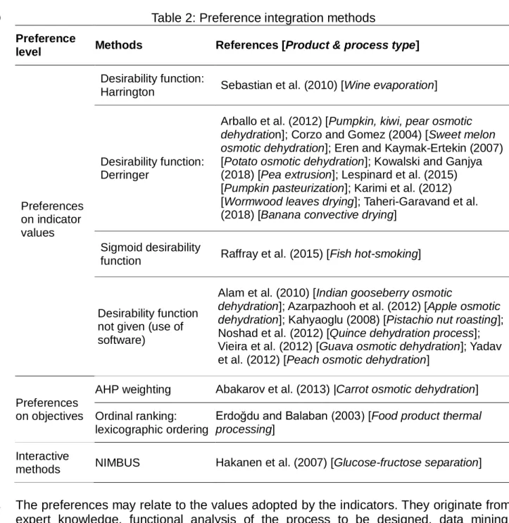
The articles reviewed in which the preferences are integrated via specific methods have 506
been classified in table 2, depending on whether the preferences are on the indicators, 507
the significance of the objectives, or whether they are integrated interactively. 508
Table 2: Preference integration methods 510
Preference
level Methods References [Product & process type]
Preferences on indicator values
Desirability function:
Harrington Sebastian et al. (2010) [Wine evaporation]
Desirability function: Derringer
Arballo et al. (2012) [Pumpkin, kiwi, pear osmotic dehydration]; Corzo and Gomez (2004) [Sweet melon osmotic dehydration]; Eren and Kaymak-Ertekin (2007) [Potato osmotic dehydration]; Kowalski and Ganjya (2018) [Pea extrusion]; Lespinard et al. (2015) [Pumpkin pasteurization]; Karimi et al. (2012) [Wormwood leaves drying]; Taheri-Garavand et al. (2018) [Banana convective drying]
Sigmoid desirability
function Raffray et al. (2015) [Fish hot-smoking]
Desirability function not given (use of software)
Alam et al. (2010) [Indian gooseberry osmotic
dehydration]; Azarpazhooh et al. (2012) [Apple osmotic dehydration]; Kahyaoglu (2008) [Pistachio nut roasting]; Noshad et al. (2012) [Quince dehydration process]; Vieira et al. (2012) [Guava osmotic dehydration]; Yadav et al. (2012) [Peach osmotic dehydration]
Preferences on objectives
AHP weighting Abakarov et al. (2013) |Carrot osmotic dehydration] Ordinal ranking:
lexicographic ordering
Erdoğdu and Balaban (2003) [Food product thermal processing]
Interactive
methods NIMBUS Hakanen et al. (2007) [Glucose-fructose separation]
511
The preferences may relate to the values adopted by the indicators. They originate from 512
expert knowledge, functional analysis of the process to be designed, data mining, 513
market studies... Their usefulness is based on: 514
Reducing the search space for possible solutions, by proposing desired valves 515
(upper and lower) associated with each indicator. This may prove particularly 516
useful in the case of raw indicators, for which context-specific limitations may be 517
integrated; thus for example in Sebastian et al. (2010), the maximum acceptable 518
mass of the equipment makes it possible to evaluate the transportability objective 519
of the equipment. 520
Favouring certain indicator values over others, by means of desirability functions. 521
Desirability functions convert the value of an indicator into a dimensionless variable of 522
between 0 and 1, known as “satisfaction index”, which quantifies the satisfaction of the 523
decision-maker on the performance of the indicator. They require the determination of a 524
high value for the indicator (associated with an upper or lower desirability value) and a 525
low value (associated with a lower or upper desirability value, respectively), in order to 526
demarcate the desirability domain. The most commonly used functions in the literature 527
(Arballo et al., 2012; Corzo and Gomez, 2004; Eren and Kaymak-Ertekin, 2007; 528
Lespinard et al., 2015) are those from Derringer (1980), one able to express increasing 529
or decreasing desirability (one-sided), and the other to express maximum desirability in 530
one domain, and decreasing when an indicator moves away from this domain (two-531
sided). There are other forms of desirability function, in various mathematical forms, 532
such as from Harrington (1965), used in Sebastian et al. (2010), and the sigmoid 533
function (Raffray et al., 2015). All these functions lead to normalized indicators 534
(expressed on a common scale), which can facilitate ranking the solutions by 535
aggregating the scores. The choice between the different existing functions depends on 536
how the desirability values are seen, as a function of the values of the indicator under 537
study. Thus for example, the functions from Derringer (1980) strictly demarcate the 538
indicator’s domain of variation, while the sigmoid function from Raffray et al. (2015) 539
remains discriminant in the vicinity of the domain under study. 540
541
The decision-maker may also formulate preferences over the relative significance of 542
their objectives, i.e. on the comparative significance of the indicators. This may involve 543
weighting the objectives, or ranking them in order of significance. If the decision-maker 544
is faced with a multitude of objectives, it may be difficult to rationally and consistently 545
attribute the weights. That is why there are methods to help the decision-maker to 546
prioritize the objectives: the AHP method (Analytic Hierarchy process – Saaty (1990)) for 547
example, which designates a method even capable of ranking the solutions, includes a 548
step of defining the weights by comparing the objectives (or indicators) in pairs, is used 549
in Abakarov et al. (2013). A score of between 1 and 9 is attributed to each objective 550
depending on its significance compared to every other objective, and the results are 551
aggregated using a given formula to provide a numerical value for the weight of each 552
objective. Other methods use pairwise comparison, a non-exhaustive list of which is 553
given in Siskos and Tsotsolas (2015). Ranking the objectives in order of significance 554
does not require priorization methods. It has been used by Erdoğdu and Balaban (2003) 555
and named “lexicographic ordering”. This approach seems uncommon, since most 556
decision-making aid and optimization methods require quantification of the significance 557
of the objectives for calculating the objective functions. Otherwise, lexicographic 558
ordering of the indicators must be implemented in the optimization algorithm, as is the 559
case in Erdoğdu and Balaban (2003). Another possibility is to use a lexicographic 560
approach to produce a weighting (Sebastian et al., 2010): the objectives are ranked by 561
significance, and a mathematical function attributes a weight to each objective according 562
to its level of significance. This approach is similar to the SMARTER method (Edwards 563
and Barron, 1994), and to other hybrid approaches of this type, such as: the Simos 564
method (Figueira and Roy, 2002; Simos, 1990a, 1990b), where cards are used to order 565
the objectives and quantify their relative significance, and the SWING method, in which 566
the objectives are ranked based on solutions with the best possible value for one 567
indicator, and the worst possible value in all the others. Interested readers can find a 568
detailed review of weighting methods in Wang et al. (2009). 569
570
Finally, there are optimization methods in which the decision-maker formulates their 571
preferences through an iterative design process, in which solutions are presented to 572
them. These so-called interactive methods generally proceed in three phases (Coello, 573
2000): 574
1. Calculate a Pareto-efficient solution; 575
2. Put together the decision-maker’s preferences on this solution, and its possible 576
improvements; 577
3. Repeat steps 1 and 2 until the decision-maker is satisfied. 578
The advantages of this type of method lie mainly in the low requirement for calculations 579
(few solutions calculated in each iteration), the absence of need for an overall 580
preferences diagram, and the possibility for the decision-maker to correct their 581
preferences and therefore learn through the optimization process (Taras and 582
Woinaroschy, 2012). Conversely, it is assumed that the decision-maker has the 583
necessary time and capacities to take part in the decision-making process, and that the 584
information supplied to the decision-maker is comprehensible and relevant (Miettinen, 585
1998). Although a substantial number of interactive optimization methods are available 586
(Collette and Siarry, 2013; Miettinen, 1998; Miettinen and Hakanen, 2009… ), only 587
Hakanen et al. (2007) have used them, with the NIMBUS method (Miettinen and 588
Mäkelä, 1995, 2006). In NIMBUS, when a solution is presented to the decision-maker, 589
the latter specifies for each indicator how they would like it to evolve - for example if an 590
indicator needs to be improved, is satisfactory, or may be downgraded - and these 591
preferences are used to converge toward the most satisfactory possible solution for the 592
decision-maker. 593
594
If the optimization problem encountered has not been solved by an interactive method, 595
the preferences integration methods (desirability functions, weighting methods and 596
ranking methods for objective) prove useful in providing a framework for formulating the 597
preferences. To this end, the desirability function best suited to the objectives to be 598
optimized must be chosen, in particular preventing an indicator from adopting 599
undesirable values. The choice of weighting method meanwhile will depend primarily on 600
the user’s affinity with one method or the other, and the ease with which they can 601
formulate their preferences. 602
5. Selection methods
603The quantified preferences of the decision-maker may then be used to select the most 604
acceptable solution for the decision-maker. So in the case of an optimization problem, 605
this involves constructing a function or a mathematical criterion able to evaluate the 606
performances of the solutions generated by the process model. Yet it is also possible 607
that the decision-maker will be unable to formulate preferences, or that they are not 608
provided, in the absence of a decision-making context for example. That is why the 609
reviewed articles are classified in two major categories: 610
“No information” (Table 3): in the absence of information from the decision-maker, 611
it is possible to calculate a relevant set of solutions (“Sorting / Filtering”), which 612
can then be compared in a decision-making context, or to select a solution 613
anyway without reference to the decision-makers formulated preferences 614
(“Ranking with weight elicitation”); 615
“Preferences expressed” (Table 4): the decision-maker’s preferences are 616
expressed, so a solution acceptable under the decision-maker’s criteria can be 617
selected. 618
Table 3: Selection methods – no information from the decision-maker 620
621 622
Table 4: Selection methods – preferences of the decision-maker(s) are expressed 623
624
5.1. No information
626
If the decision-maker’s preferences cannot be formulated, the approach most commonly 627
used in the literature is obtaining the Pareto front, i.e. a larger or smaller set of non-628
dominated solutions. The concept of Pareto efficiency or dominance is illustrated in 629
figure 2, where the Pareto front covers all the solutions which are not inferior to any 630
solution at any point (i.e. for each indicator). Thus many authors have opted for this 631
approach (Abakarov et al., 2009; Kiranoudis and Markatos, 2000; Kopsidas, 1995; 632
Massebeuf et al., 1999; Nishitani and Kunugita, 1979…) for the purpose of providing 633
Pareto efficient design solutions uncoupled from any context, on which a decision-maker 634
can formulate their preferences. So there is no bias, hence it is possible to optimize 635
without a priori knowledge of the decision-maker’s preferences (Massebeuf et al., 1999), 636
since an initial sort is carried out by eliminating the dominated solutions. However, this 637
method entails the risk of generating a large number of Pareto-efficient solutions 638
(Raffray et al., 2015), or even absurd solutions for the decision-maker, due to the low 639
solution filtering capacity (Scott and Antonsson, 1998). Indeed, a solution which is 640
extremely poor under one of the indicators may be among the non-dominated solutions, 641
but could be useless as a design solution. In addition, as identified by several authors 642
(Hadiyanto et al., 2009; Hakanen et al., 2007; Subramani et al., 2003), Pareto efficient 643
solutions may be presented to the decision-maker in graphic form for two or three 644
indicators, but interpretation becomes difficult after three. 645
646
647 648
Figure 2: Graphic representation of a Pareto front for two indicators (yi and yj). The solutions are designated by the
Another possibility, making it possible to go beyond the Pareto front while maintaining as 649
neutral an approach as possible, is to use an aggregation function which eliminates 650
weighting of the objectives (“weight elicitation” - Wang et al. (2009)). Thus it is possible 651
to calculate the weighted sum, definitely one of the simplest and most commonly used 652
aggregation functions, with the normalized indicators, assuming equal weight for each 653
indicator. In Erdoğdu and Balaban (2003), the weighted sum became a simple “objective 654
sum” (Marler and Arora, 2004). Another neutral function, the geometric mean, is used in 655
several works (Corzo and Gomez, 2004; Kahyaoglu, 2008; Vieira et al., 2012). Product 656
aggregation functions, like the geometric mean, are said to be more “aggressive” than 657
sum functions (Quirante, 2012), since a low value for one indicator will have a big impact 658
on the total score, and consequently better discrimination of the compromise solutions. 659
Another possible approach is calculating the distance (Euclidian distance, with two or 660
more dimensions) from “utopian” or “ideal” solutions; in the TOPSIS method (“Technique 661
for Order Preference by Similarity to Ideal Solution”) used in Madoumier (2016), the 662
solutions are ranked by a function which aggregates the distance of a given solution 663
from the “ideal” solution (comprising the best values for each indicator) and from the 664
“anti-ideal” solution (comprising the worst values for each indicator), with the best 665
solutions evidently being the closest to the former and the furthest from the latter. A 666
shortcoming of these aggregation functions is their compensatory logic, i.e. a high value 667
for one indicator may counterbalance a low value for another indicator (Collignan, 2011). 668
To offset this shortcoming, there are so-called “conservative” aggregation functions (Otto 669
and Antonsson, 1991), such as minimum aggregation (Raffray et al., 2015): the score of 670
a solution is represented by the lowest value among its indicators. So maximizing this 671
score comes down to selecting the “least worst” of all the solutions. According to the 672
same logic, maximum aggregation gives the score of a solution as being the best value 673
among its indicators, but this logic is not suited to a design context (Scott and 674
Antonsson, 1998). 675
5.2. Preferences expressed
676
If the decision-maker’s preferences are expressed, they can be used to more finely filter 677
a set of solutions. Within the framework of RSM modelling (Response Surface 678
Methodology), a graphic method of filtering the response surfaces was developed by 679
Lind et al. (1960): the overlaid contour plots method comprises overlaying the contour 680
plots for the various indicators, the value of which is determined according to the 681
decision-maker’s preferences, in order to isolate a zone in which the indicator values are 682
most satisfactory. Used with success by several authors (Annor et al., 2010; Collignan 683
and Raoult-Wack, 1994; Ozdemir et al., 2008; Singh et al., 2010), this graphic method 684
does however lose some efficiency when the number of design variables is greater than 685
two (Khuri and Mukhopadhyay, 2010), and when the optimization requirements are more 686
complex (Myers et al., 2016). Some authors (Alam et al., 2010; Arballo et al., 2012) use 687
in addition an MADM based on desirability functions to select the best solution from 688
those filtered. Another method, this time based on using tables (known as the “Tabular 689
method”), is used in Abakarov et al. (2013). Its principle is to rank the values adopted by 690
each indicator according to whether they must be maximized or minimized. Hence each 691
row in the table no longer corresponds to one solution. This then enables the decision-692
maker’s preferences to be applied to the indicators to eliminate the undesirable values. 693
If the remaining values correspond to proposed solutions, these are adopted. The risk 694
with this type of approach is that if there is no solution corresponding to the preferences 695
on the indicators, it forces the decision-maker to revise their requirements downward. 696
697
To obtain a ranking of solutions or select the best compromise, the decision-maker’s 698
preferences may be integrated into the aforementioned aggregation functions, in the 699
form of weighting. The most classic are the weighted sum, used in Asgari et al. (2017), 700
Hadiyanto et al. (2008a; 2008b) and Sidaway and Kok (1982), and the weighted 701
geometric mean (or weighted product) used in four studies (Arballo et al., 2012; Eren 702
and Kaymak-Ertekin, 2007; Lespinard et al., 2015; Sebastian et al., 2010). Proposed by 703
Derringer (1994), the geometric mean is used in the four studies to aggregate 704
normalized indicators by means of desirability functions. A potential shortcoming of the 705
weighted geometric mean is that the meaning given to the weights is less intuitive than 706
in a weighted sum, since the indicators between them have an exponential relative 707
significance instead of a proportional relative significance (Collignan, 2011). However, it 708
makes it possible to eliminate solutions where an indicator adopts a very low value or 709
zero, under an “aggressive” strategy as mentioned above. Besides these “primary” 710
aggregation functions (as per Marler and Arora (2004)), it is possible to adopt more 711
complex aggregation strategies, at least two of which have been identified within this 712
work: 713
Integration strategy within a more complex decision-making aid framework, such 714
as the AHP method employed in Abakarov et al. (2013): the steps for determining 715
the weights, set out in section 4, lead to a weighted sum aggregation. 716
“Mathematical” strategy, aimed at increasing the complexity of the aggregation 717
functions. An example is the function derived from an optimization method known 718
as “loss-minimization method” (Equation 1), corresponding to the weighted sum 719
(weight wi) of variables defined as the relative difference between an indicator
720
(Qi) and its optimal value (Qi*) (Gergely et al., 2003). This function requires prior
721
single-objective optimization of the indicators, to obtain their optimal value. 722 723 724 725 726 727
The aggregation functions mentioned above belong to full aggregation approaches, 728
characterized by the synthesis of several indicators into a single score, which can be 729
distinguished from so-called partial aggregation approaches or outranking approaches 730
(Brans and Vincke, 1985). The latter are based on construction of binary relationships 731
between solutions, based on the decision-maker’s preferences (Wang et al., 2009). 732
Hence it is possible to do without an overall aggregation function, but it is also 733
necessary to be able to compare the solutions in twos. This means that partial 734
aggregation methods are applicable only when a sufficiently small set of solutions has 735
been generated. Thus in Massebeuf et al. (1999), the best solution is selected after 736
obtaining Pareto efficient solutions. The partial aggregation method employed in 737
Massebeuf et al. (1999) is constructed from methods such as ELECTRE (Elimination 738
and choice translating reality) and PROMETHEE (Preference ranking organization 739
method for enrichment evaluation); these two terms represent method families suited to 740
various types of issue (sorting for Electre-Tri, choice for ELECTRE I and PROMETHEE 741
I, ranking for ELECTRE III and PROMETHEE II, …), the general principles of which are 742
in brief: 743
ELECTRE (Roy, 1968) provides a ranking or preference relationships between 744
solutions, without calculating a cardinal score, based on concordance & 745
discordance indices, and threshold values (Wang et al., 2009). The relationships 746
between solutions are obtained based on pair comparison under each of the 747
decision-maker’s objectives. 748
PROMETHEE (Brans and Vincke, 1985) is based on quantified comparison of 749
solutions, i.e. the relationship between solutions under a given indicator will be 750
described by a preference function evaluating the intensity of this preference. 751
This information is used to calculate the “incoming” and “outgoing” flows of a 752
solution, i.e. the quantitative measurement of confidence and regret, respectively, 753
relating to a solution (Wang et al., 2009). 754
For selection or ranking issues, methods such as PROMETHEE are deemed easier to 755
use than methods such as ELECTRE (Velasquez and Hester, 2013), and were indeed 756
designed as an improvement on the latter (Brans and Vincke, 1985). 757
758
5.3. Normalization
759
A question rarely addressed, concerning the application (or possible development) of 760
selection methods, is that of normalization. Most of these methods require normalization 761
of the indicators to enable their comparison on a common scale; if normalization is not 762
applied by a desirability function, simple mathematical operators are applied, such as 763
division by an optimum or a reference value. Yet the works of Pavličić (2001) indicate 764
that the selection results may depend on the mathematical operation applied, and that 765
use of vector type normalization (Equation 2 – xij is the value of the jth indicator for
766
solution i, and ij is the corresponding normalized indicator) should be reconsidered. So it
767
seems that the normalization operator must be wisely chosen for the applying the 768
selection methods. 769
770 771
5.4. Difficulty of choosing a selection method
772
In view of these technical considerations and noting the diversity of approaches, the 773
question of choosing a selection method is potentially complex. Indeed, the diversity of 774
solution selection methods, and more generally MADMs, is accentuated by possible 775
combinations between methods. For example in Abakarov et al. (2013), the AHP method 776
and tabular method are combined, and in Massebeuf et al. (1999), the Pareto front is 777
filtered by a partial aggregation method, constructed with the elements of two well-778
known methods. While none of the methods appears to be the best, their respective 779
advantages and shortcomings may make them incompatible with certain applications 780