Analysis of Thermal Diodes Enabled by
Junctions of Phase Change Materials
The MIT Faculty has made this article openly available. Please sharehow this access benefits you. Your story matters.
Citation Cottrill, Anton L., and Michael S. Strano. “Analysis of Thermal Diodes Enabled by Junctions of Phase Change Materials.” Adv. Energy Mater. 5, no. 23 (September 10, 2015): n/a–n/a.
As Published http://dx.doi.org/10.1002/aenm.201500921
Publisher Wiley Blackwell
Version Author's final manuscript
Citable link http://hdl.handle.net/1721.1/102318
Terms of Use Creative Commons Attribution-Noncommercial-Share Alike
DOI: 10.1002/aenm.201500921 Article type: Full Paper
Analysis of Thermal Diodes Enabled by Junctions of Phase Change Materials
Anton L. Cottrill and Michael S. Strano*
A. L. Cottrill, Prof. M. S. Strano Department of Chemical Engineering Massachusetts Institute of Technology Cambridge, MA 02139, USA
E-mail: strano@mit.edu
Keywords: thermal rectification, thermal diodes, phase change materials
Materials designed to undergo a phase transition at a prescribed temperature have been advanced as elements for controlling thermal flux. Such phase change materials can be used as components of reversible thermal diodes, or materials that favor heat flux in a preferred direction; however, a thorough mathematical analysis of such diodes is thus far absent from the literature. Herein, it is shown mathematically that the interface of a phase change material with a phase invariant one can function as a simple thermal diode. Design equations are derived for such phase change diodes, solving for the limits where the transition temperature falls within or outside of the temperature gradient across the device. Criteria are derived analytically for the choice of thermal conductivity of the invariant phase to maximize the rectification ratio. Finally, the model is applied to several
experimental systems in the literature, providing bounds on observed performance. This model should aid in the development of materials capable of controlling heat flux.
1. Introduction
A thermal rectifier, the thermal analog to the electrical diode, is a device characterized by a preferential direction for heat flow.[1] The degree of thermal rectification is typically quantified under steady state conditions. It is equal to the ratio of the magnitudes of forward heat flux and reverse heat flux under forward and reverse temperature bias conditions of identical magnitudes, respectively.
We can consider a 1-D system in contact with a hot temperature boundary condition, 𝑇𝑇𝐻𝐻, on one side and a cold temperature boundary condition, 𝑇𝑇𝐶𝐶, on the opposing side. This temperature bias will provide a steady state heat flux, 𝑞𝑞+, in the direction from 𝑇𝑇𝐻𝐻 to 𝑇𝑇𝐶𝐶. A reversal of the temperature bias, while maintaining its magnitude, yields the steady state heat flux, 𝑞𝑞−, in the opposite direction. In the case of a thermal rectifying device, the magnitudes of these two heat fluxes will be unequal, and their ratio is termed the rectification ratio, 𝑄𝑄.
An asymmetrical thermal conductance was first recognized experimentally at the interface of copper and copper oxide in 1936 by Starr et al.[2] The phenomenon of thermal rectification has paved the way for the field of phononics[1] via the development of thermal transistors,[3-6] thermal logic circuits,[7] and thermal memory.[8] Furthermore, thermal diodes have a vast array of applications in the fields of nano-scale and micro-nano-scale heat management.[9,10] Various strategies have been implemented for experimentally demonstrating a thermal rectifier. Researchers have applied electronic principles, such as semiconductor technology, towards thermal diode design.[2,11-12] In addition, the incorporation of geometric asymmetries into nano-structured, micro-structured, and bulk devices has yielded promising results.[13-17] The manipulation of contact areas between interfaces, due to thermal warping, has also proven successful as a thermal diode design.[10]
A promising method for developing a device with thermal rectification is to introduce a non-linear element, such as a material with a temperature-dependent thermal conductivity, into the system. Furthermore, in order to break the symmetry imposed by the boundary conditions, an additional
element, linear or non-linear, should be interfaced with the non-linear element, introducing a space dependency for thermal conductivity. Mathematically, this corresponds to transforming the system’s steady state energy balance from a linear autonomous differential equation to a linear non-autonomous differential equation. For example, a device composed of a material with a dependent thermal conductivity (non-linear element) interfaced with a material with a temperature-independent thermal conductivity (linear element) would satisfy these constraints. Ideally, it is envisioned that the two interfaced materials would have opposing trends in thermal conductivity as a function of temperature. Experimental observations of thermal rectification due to interfaces between materials of different thermal conductivity temperature dependencies date to the 1970s.[18-20] Current examples of thermal rectifiers that incorporate this design have been demonstrated experimentally by Takeuchi et al. and Kobayashi et al., achieving rectification ratios up to 1.43.[15, 21-22]
Several strides have been made towards the numerical and analytical modeling of these non-linear systems at steady state. M. Peyrard analyzed such a system with basic continuum laws of heat conduction.[23] He proposed modelling the steady state thermal diode system with a linear non-autonomous differential equation. The system’s rectification ratio can then be calculated through self-consistent iteration, provided data for the materials’ thermal conductivities as a function of temperature are available. It should be noted that Kobayashi et al. used this numerical approach to calculate the theoretically predicted rectification ratios of their system, which agreed well with their experimental values.[15, 21] Hu et al. simulated such a thermal diode system by performing Hamiltonian mechanics calculations of coupled 𝜑𝜑4 and Frenkel-Kontorova lattices, in order to simulate the opposing trends of thermal conductivity with respect to temperature.[24] On a similar note, researchers have also modeled coupled segments with different thermal conductivity temperature dependencies with two-dimensional asymmetrical Ising models.[25] C. Dames developed an analytical model for this two-segment system by approximating the thermal conductivities with power law expressions and solving the resulting
differential equations with perturbation analysis. The analysis agreed well with experimental results in literature and provided more insight towards the design of such devices.[26]
Employing phase change materials to obtain a variation in physical properties with respect to temperature is an emerging avenue for designing thermal diodes.[27-30] Recently, a thermal diode was developed with a two-segment design consisting of nitinol and graphite. Nitinol, a nickel titanium alloy, undergoes a change in thermal conductivity as the material transitions between the austenite and martensite crystal structures. Researchers have reported experimental thermal rectification ratios up to 1.47 for such a device.[27] A concept for a phase-change radiative thermal diode has also been proposed.[28] A two-segment device consisting of poly(N-isopropylacrylamide) (PNIPAM), a phase-changing polymer, and polydimethylsiloxane (PDMS) has also been demonstrated to show thermal rectification. Below the lower-critical-solution-temperature (LCST) of the PNIPAM polymer, water is immobilized throughout the polymer. However, above the LCST the water exits the polymer, which changes its configuration and reduces its size. In this case, the thermal conductivity of the PNIPAM does not necessarily alter. Rather, the effective thermal conductivity of the composite system changes, yielding thermal rectification when interfaced with PDMS, which has a temperature-independent thermal conductivity. A simple model based on a smooth step change in effective thermal resistance with respect to temperature for the PNIPAM was proposed by the researchers to model the system. This model was analyzed numerically, and it yielded thermal rectification estimates close to the experimental values obtained.[29]
The intent of this paper is to further the understanding of thermal rectifying devices that are based on changes in thermal conductivity due to phase transitions. A simple, analytical model based on continuum laws of heat conduction at steady state will be proposed for understanding the relevant thermal resistances for device optimization. Furthermore, this model will be applied to experimental data existing in the literature and compared to numerical calculations based on the method outlined by
M. Peyrard.[23] Finally, this model will be used to elucidate optimal design strategies for other potential phase change thermal diodes based on data present in the literature.
2. Problem Statement
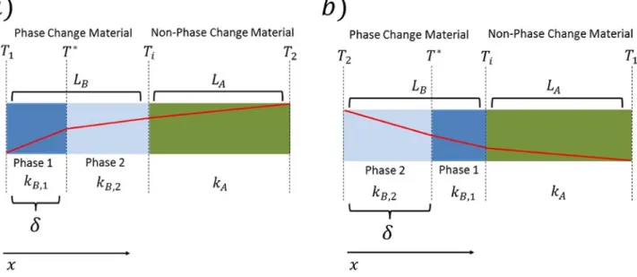
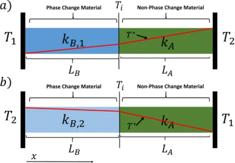
Consider the junction of two 1-D materials A and B, of lengths 𝐿𝐿𝐴𝐴 and 𝐿𝐿𝐵𝐵, respectively, and with material B possessing a first-order phase transition at temperature 𝑇𝑇∗ from phase B1 at a temperature below 𝑇𝑇∗ to phase B2 at a temperature above 𝑇𝑇∗. For simplicity, we refer to A as the invariant material, having no phase transition for all 𝑇𝑇. The temperature-dependent thermal conductivity of material A is 𝑘𝑘𝐴𝐴(𝑇𝑇) while B has thermal conductivity 𝑘𝑘𝐵𝐵,1(𝑇𝑇) for phase 1 and 𝑘𝑘𝐵𝐵,2(𝑇𝑇) for phase 2. We analyze the case where this material is temperature-controlled, such that the external boundary of A is maintained isothermally at T2 while the external boundary of B is at T1, and the heat flux in the system reaches a stationary state. Figure 1a depicts the physical schematic of the junction of materials A and B. We first assume that 𝑇𝑇1 < 𝑇𝑇∗ < 𝑇𝑇2, and in the case of Figure 1a, this implies that phase B1 is the low temperature phase, transitioning to phase B2 upon heating the system above 𝑇𝑇∗. We therefore anticipate a phase boundary at a distance δ from the external B interface as shown in Figure 1a, which varies with 𝑇𝑇1 and 𝑇𝑇2, the lengths of each material, 𝐿𝐿𝐴𝐴 and 𝐿𝐿𝐵𝐵, and the thermal properties of the composite system.
Fourier’s Law for material A and for each phase of material B at steady state is as follows:
𝜕𝜕 𝜕𝜕𝜕𝜕 � 𝑘𝑘𝐴𝐴(𝑇𝑇) 𝜕𝜕𝜕𝜕 𝜕𝜕𝜕𝜕� = 0 (1) 𝜕𝜕 𝜕𝜕𝜕𝜕 � 𝑘𝑘𝐵𝐵,1(𝑇𝑇) 𝜕𝜕𝜕𝜕 𝜕𝜕𝜕𝜕� = 0 (2) 𝜕𝜕 𝜕𝜕𝜕𝜕 � 𝑘𝑘𝐵𝐵,2(𝑇𝑇) 𝜕𝜕𝜕𝜕 𝜕𝜕𝜕𝜕� = 0 (3)
The heat flux through the 1-D system must be invariant at steady state, such that:
𝑘𝑘𝐴𝐴(𝑇𝑇)𝜕𝜕𝜕𝜕 𝜕𝜕𝜕𝜕 = 𝑘𝑘𝐵𝐵,1(𝑇𝑇) 𝜕𝜕𝜕𝜕 𝜕𝜕𝜕𝜕 = 𝑘𝑘𝐵𝐵,2(𝑇𝑇) 𝜕𝜕𝜕𝜕 𝜕𝜕𝜕𝜕 = −𝑞𝑞 (4)
With 𝑥𝑥 = 0 taken as the external B interface, the boundary conditions become: 𝑇𝑇(𝑥𝑥 = 0) = 𝑇𝑇1 (5)
𝑇𝑇(𝑥𝑥 = 𝛿𝛿) = 𝑇𝑇∗ (6)
𝑇𝑇(𝑥𝑥 = 𝐿𝐿𝐵𝐵) = 𝑇𝑇𝑖𝑖 (7)
𝑇𝑇(𝑥𝑥 = 𝐿𝐿𝐴𝐴 + 𝐿𝐿𝐵𝐵) = 𝑇𝑇2 (8)
where 𝑇𝑇𝑖𝑖 is the interfacial temperature between materials A and B. Equal thermal flux boundary conditions existing at the interface between the two phases of material B and the interface between materials A and B are also applied.
In order to quantify the magnitude of thermal rectification, the reversal of the temperature boundary conditions shown in Figure 1a needs to be considered. A reversal of these temperature boundary conditions yields Figure 1b. The ratio of the magnitudes of the thermal fluxes between the two systems described in Figure 1 yields the thermal rectification ratio for this system. Mathematically predicting the magnitude of thermal rectification can be approached analytically or numerically, as presented below.
2.1. Case I: Constant Thermal Conductivities and {δ: 0 < δ < LB}
The type of diode of primary consideration in this work is one enabled by the change of phase of B. Such a phase change diode can operate if 𝑇𝑇1 < 𝑇𝑇∗< 𝑇𝑇2. For Case I, we further restrict the analysis to conditions such that {δ: 0 < δ < LB}. We consider the case of constant thermal conductivity for simplicity, noting that it applies in general for a diode operating about the temperature 𝑇𝑇∗ with a
relatively small-applied temperature gradient. Non-constant thermal conductivities can be treated in a manner described below in Case III.
In this case, the linear temperature profiles for domains A, B1, and B2 for the system illustrated in Figure 1a are: 𝑇𝑇𝐴𝐴(𝑥𝑥) = �𝜕𝜕2−𝜕𝜕𝑖𝑖 𝐿𝐿𝐴𝐴 � (𝑥𝑥 − 𝐿𝐿𝐵𝐵) + 𝑇𝑇𝑖𝑖 (9) 𝑇𝑇𝐵𝐵,1(𝑥𝑥) = �𝜕𝜕∗−𝜕𝜕1 𝛿𝛿 � 𝑥𝑥 + 𝑇𝑇1 (10) 𝑇𝑇𝐵𝐵,2(𝑥𝑥) = �𝜕𝜕𝑖𝑖−𝜕𝜕∗ 𝐿𝐿𝐵𝐵−𝛿𝛿� (𝑥𝑥 − 𝛿𝛿) + 𝑇𝑇 ∗ (11)
The interfacial temperature 𝑇𝑇𝑖𝑖 is a function of thermophysical properties and applied temperatures:
𝑇𝑇𝑖𝑖 = − �𝑘𝑘𝐵𝐵,2(𝜕𝜕2−𝜕𝜕∗)+𝑘𝑘𝐵𝐵,1(𝜕𝜕∗−𝜕𝜕1)
𝑘𝑘𝐴𝐴𝐿𝐿𝐵𝐵+𝑘𝑘𝐵𝐵,2𝐿𝐿𝐴𝐴 � 𝐿𝐿𝐴𝐴 + 𝑇𝑇2 (12)
while the phase boundary in B appears at:
δ1−2 =𝑘𝑘𝐵𝐵,1 𝑘𝑘𝐴𝐴
(𝜕𝜕∗−𝜕𝜕1)(𝑘𝑘𝐴𝐴𝐿𝐿𝐵𝐵+𝑘𝑘𝐵𝐵,2𝐿𝐿𝐴𝐴)
𝑘𝑘𝐵𝐵,2(𝜕𝜕2−𝜕𝜕∗)+𝑘𝑘𝐵𝐵,1(𝜕𝜕∗−𝜕𝜕1) (13)
where the subscript 1-2 indicates the direction of the imposed temperature gradient, as evidenced by the locations of 𝑇𝑇1 and 𝑇𝑇2.
The magnitude of the steady flux through this system is then:
|𝑞𝑞1−2| = 𝑘𝑘𝐴𝐴�𝑘𝑘𝐵𝐵,2(𝜕𝜕2−𝜕𝜕∗)+𝑘𝑘𝐵𝐵,1(𝜕𝜕∗−𝜕𝜕1)
𝑘𝑘𝐴𝐴𝐿𝐿𝐵𝐵+𝑘𝑘𝐵𝐵,2𝐿𝐿𝐴𝐴 � (14)
where the subscript 1-2 indicates the direction of the imposed temperature gradient, as evidenced by the locations of 𝑇𝑇1 and 𝑇𝑇2.
If we consider the flux in the opposing direction, should 𝑇𝑇1 be applied instead to the 𝑥𝑥 = 𝐿𝐿𝐴𝐴 + 𝐿𝐿𝐵𝐵 boundary, and 𝑇𝑇2 applied to 𝑥𝑥 = 0 boundary, we note that the ordering of the phases necessarily changes to that of Figure 1b. Specifically, phase 𝐵𝐵2, and not phase 𝐵𝐵1, becomes the external boundary for the B domain. From symmetry, we can set 𝑇𝑇1 → 𝑇𝑇2 and 𝑘𝑘𝐵𝐵,1 → 𝑘𝑘𝐵𝐵,2 to find the opposing flux under this condition:
|𝑞𝑞2−1| = 𝑘𝑘𝐴𝐴�𝑘𝑘𝐵𝐵,1(𝜕𝜕∗−𝜕𝜕1)+𝑘𝑘𝐵𝐵,2(𝜕𝜕2−𝜕𝜕∗)
𝑘𝑘𝐴𝐴𝐿𝐿𝐵𝐵+𝑘𝑘𝐵𝐵,1𝐿𝐿𝐴𝐴 � (15)
Interestingly, the rectification ratio becomes:
𝑄𝑄 =|𝑞𝑞1−2| |𝑞𝑞2−1|=
𝑘𝑘𝐴𝐴𝐿𝐿𝐵𝐵+𝑘𝑘𝐵𝐵,1𝐿𝐿𝐴𝐴
𝑘𝑘𝐴𝐴𝐿𝐿𝐵𝐵+𝑘𝑘𝐵𝐵,2𝐿𝐿𝐴𝐴 (16)
The model proposed above is valid under the following circumstances:
0 < 𝛿𝛿1−2< 𝐿𝐿𝐵𝐵 𝑎𝑎𝑎𝑎𝑎𝑎 0 < 𝛿𝛿2−1< 𝐿𝐿𝐵𝐵 (17)
Application of these inequalities yields constraints for the validity of the model:
𝑘𝑘𝐴𝐴 𝑘𝑘𝐵𝐵,2 > 𝐿𝐿𝐴𝐴 𝐿𝐿𝐵𝐵 (𝜕𝜕∗−𝜕𝜕 2) (𝜕𝜕1−𝜕𝜕∗) (from 𝛿𝛿2−1) (18) 𝑘𝑘𝐴𝐴 𝑘𝑘𝐵𝐵,1> 𝐿𝐿𝐴𝐴 𝐿𝐿𝐵𝐵 (𝜕𝜕∗−𝜕𝜕1) (𝜕𝜕2−𝜕𝜕∗) (from 𝛿𝛿1−2) (19)
Therefore, when the thermophysical properties and applied temperature gradient satisfy Equation (18) and (19), Equation (16) can be used to predict the thermal rectification ratio for the system. For systems in which the applied temperature gradient and thermophysical properties yield 𝛿𝛿 ≥ 𝐿𝐿𝐵𝐵, indicating the absence of a phase boundary, a different model needs to be considered. The parameter 𝛿𝛿 was originally defined as the distance from the external B interface at which a phase boundary occurs. Physically, a phase boundary cannot exist at 𝛿𝛿 ≥ 𝐿𝐿𝐵𝐵 because this is in the domain of material A. This
constraint should then be physically interpreted as the position in the composite material at which the temperature is 𝑇𝑇∗.
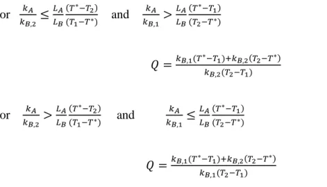
2.2. Case II: Constant Thermal Conductivities and {δ: δ ≥ LB}
Under certain conditions, the phase change material will exist as a single phase under both sets of temperature boundary conditions (1-2 and 2-1). In other words, for certain systems and boundary conditions, there will be no phase change boundaries within the phase transition material. Figure 2 qualitatively illustrates the thermal conductivity distributions of such a system for a general set of temperature boundary conditions. This system can be analyzed as a combination of linear systems, which have a change in thermal conductivity of the phase change material upon reversal of the temperature bias. A steady state solution for this linear system can be obtained by applying the appropriate temperature boundary conditions at the ends of the two-segment system and equal temperature and equal thermal flux constraints at the interface. Equation (20) and (21) are the temperature profiles for the phase change material and the invariant material, respectively, under the temperature bias shown in Figure 2a.
𝑇𝑇𝐵𝐵(𝑥𝑥) =(𝜕𝜕𝑖𝑖−𝜕𝜕1)
𝐿𝐿𝐵𝐵 𝑥𝑥 + 𝑇𝑇1 (20)
𝑇𝑇𝐴𝐴(𝑥𝑥) =(𝜕𝜕2−𝜕𝜕𝑖𝑖)
𝐿𝐿𝐴𝐴 (𝑥𝑥 − 𝐿𝐿𝐵𝐵) + 𝑇𝑇𝑖𝑖 (21)
Again, the interfacial temperature 𝑇𝑇𝑖𝑖 is a function of thermophysical properties and applied temperatures:
𝑇𝑇𝑖𝑖 = 𝑘𝑘𝐴𝐴𝐿𝐿𝐵𝐵𝜕𝜕2+𝑘𝑘𝐵𝐵,1𝐿𝐿𝐴𝐴𝜕𝜕1
𝑘𝑘𝐵𝐵,1𝐿𝐿𝐴𝐴+𝑘𝑘𝐴𝐴𝐿𝐿𝐵𝐵 (22)
The magnitude of the steady state flux though the system is then:
|𝑞𝑞1−2| =𝑘𝑘𝐴𝐴𝑘𝑘𝐵𝐵,1(𝜕𝜕2−𝜕𝜕1)
𝑘𝑘𝐴𝐴𝐿𝐿𝐵𝐵+𝑘𝑘𝐵𝐵,1𝐿𝐿𝐴𝐴 (23)
where the subscript 1-2 indicates the direction of the imposed temperature gradient, as evidenced by the locations of 𝑇𝑇1 and 𝑇𝑇2.
If we consider the flux in the opposing direction, should 𝑇𝑇1 be applied instead to the 𝑥𝑥 = 𝐿𝐿𝐴𝐴 + 𝐿𝐿𝐵𝐵 boundary, and 𝑇𝑇2 applied to 𝑥𝑥 = 0 boundary, we note that the ordering of the phases necessarily changes to that of Figure 2b. From symmetry, we can set 𝑇𝑇1 → 𝑇𝑇2 and 𝑘𝑘𝐵𝐵,1 → 𝑘𝑘𝐵𝐵,2 to find the opposing flux:
|𝑞𝑞2−1| =𝑘𝑘𝐴𝐴𝑘𝑘𝐵𝐵,2(𝜕𝜕2−𝜕𝜕1)
𝑘𝑘𝐴𝐴𝐿𝐿𝐵𝐵+𝑘𝑘𝐵𝐵,2𝐿𝐿𝐴𝐴 (24)
The rectification ratio is then given by Equation (25), which is a result supported by recent analytical work performed by Zhang et al.[30]
𝑄𝑄 =|𝑞𝑞1−2| |𝑞𝑞2−1|=
𝑘𝑘𝐵𝐵,1(𝑘𝑘𝐵𝐵,2𝐿𝐿𝐴𝐴+𝑘𝑘𝐴𝐴𝐿𝐿𝐵𝐵)
𝑘𝑘𝐵𝐵,2(𝑘𝑘𝐵𝐵,1𝐿𝐿𝐴𝐴+𝑘𝑘𝐴𝐴𝐿𝐿𝐵𝐵) (25)
Again, Equation (25) can only be applied to determine the thermal rectification of the system if 𝛿𝛿 ≥ 𝐿𝐿𝐵𝐵 for both sets of boundary conditions. In other words, the following inequalities must be satisfied in order to apply this model:
𝑘𝑘𝐴𝐴 𝑘𝑘𝐵𝐵,2 ≤ 𝐿𝐿𝐴𝐴 𝐿𝐿𝐵𝐵 (𝜕𝜕∗−𝜕𝜕2) (𝜕𝜕1−𝜕𝜕∗) (from 𝛿𝛿2−1) (26) 𝑘𝑘𝐴𝐴 𝑘𝑘𝐵𝐵,1≤ 𝐿𝐿𝐴𝐴 𝐿𝐿𝐵𝐵 (𝜕𝜕∗−𝜕𝜕1) (𝜕𝜕2−𝜕𝜕∗) (from 𝛿𝛿1−2) (27)
It can be envisioned that certain thermophysical properties and temperature boundary conditions will exist for a device such that for one set of boundary conditions the temperature profile will be appropriately modeled by Equation (9-13), while the reverse boundary conditions will be appropriately
modeled with Equation (20-22). Under these circumstances, neither Equation (16) nor Equation (25) is valid to predict the thermal rectification ratio for the system. The thermal rectification ratio for these systems can be calculated by mixing the models proposed in Case I and Case II.
For 𝑘𝑘𝐴𝐴 𝑘𝑘𝐵𝐵,2≤ 𝐿𝐿𝐴𝐴 𝐿𝐿𝐵𝐵 (𝜕𝜕∗−𝜕𝜕2) (𝜕𝜕1−𝜕𝜕∗) and 𝑘𝑘𝐴𝐴 𝑘𝑘𝐵𝐵,1 > 𝐿𝐿𝐴𝐴 𝐿𝐿𝐵𝐵 (𝜕𝜕∗−𝜕𝜕1) (𝜕𝜕2−𝜕𝜕∗) 𝑄𝑄 =𝑘𝑘𝐵𝐵,1(𝜕𝜕∗−𝜕𝜕1)+𝑘𝑘𝐵𝐵,2(𝜕𝜕2−𝜕𝜕∗) 𝑘𝑘𝐵𝐵,2(𝜕𝜕2−𝜕𝜕1) (28) For 𝑘𝑘𝐴𝐴 𝑘𝑘𝐵𝐵,2 > 𝐿𝐿𝐴𝐴 𝐿𝐿𝐵𝐵 (𝜕𝜕∗−𝜕𝜕 2) (𝜕𝜕1−𝜕𝜕∗) and 𝑘𝑘𝐴𝐴 𝑘𝑘𝐵𝐵,1 ≤ 𝐿𝐿𝐴𝐴 𝐿𝐿𝐵𝐵 (𝜕𝜕∗−𝜕𝜕 1) (𝜕𝜕2−𝜕𝜕∗) 𝑄𝑄 =𝑘𝑘𝐵𝐵,1(𝜕𝜕∗−𝜕𝜕1)+𝑘𝑘𝐵𝐵,2(𝜕𝜕2−𝜕𝜕∗) 𝑘𝑘𝐵𝐵,1(𝜕𝜕2−𝜕𝜕1) (29)
Table 1 summarizes the results for the estimation of the thermal rectification ratio as a function of the thermophysical system properties and the applied temperature gradient.
2.3. Case III: Non-Constant Thermal Conductivities
The system illustrated in Figure 1 has constant thermal conductivities as a function of temperature for material A and the two phases of material B. This system can be modeled as a combination of linear conducting elements. However, if a temperature-dependent thermal conductivity is present for material A or either of the phases for material B, numerical computation is required. Additionally, one can exclude from consideration the operation of the device in Figure 1 under conditions such that material B exists only in phase B1 (𝑇𝑇1, 𝑇𝑇2 < 𝑇𝑇∗) or exists only in phase B2 (𝑇𝑇1, 𝑇𝑇2 > 𝑇𝑇∗), since thermal rectification does not occur. However, if non-constant thermal conductivities are present, thermal rectification can exist in these limits. This is the basis for the thermal diodes demonstrated experimentally by Kobayashi et al. and Takeuchi et al.[21-22] These devices need to be modeled numerically, unless the temperature dependencies of the thermal conductivity can be approximated
with power laws – a case in which the system can be modeled analytically by the method developed by C. Dames.[26] The method for numerically modeling such systems is described below, as developed by M. Peyrard.[23]
For a system at steady state, with a space-dependent, temperature-dependent, and isotropic thermal conductivity, the energy balance is as follows:
∇ ∙ (𝑘𝑘(𝑇𝑇(𝒙𝒙), 𝒙𝒙) ∇𝑇𝑇(𝑥𝑥)) = 0 (30)
where 𝑘𝑘 refers to the thermal conductivity, 𝑇𝑇 refers to the temperature, and 𝒙𝒙 refers to the position vector of the system. For a 1-D system Equation (30) can be simplified:
𝐽𝐽 = 𝑘𝑘(𝑇𝑇(𝑥𝑥), 𝑥𝑥)𝑑𝑑𝜕𝜕
𝑑𝑑𝜕𝜕 (31)
where 𝐽𝐽 is the thermal flux due to conduction. The numerical analysis proposed by M. Peyrard employs an alternative form of Equation (31) in order to solve for the thermal rectification and temperature profile of a system:[23]
𝑇𝑇(𝑥𝑥) − 𝑇𝑇(0) = ∫ 𝐽𝐽
𝑘𝑘(𝜕𝜕(𝜕𝜕′),𝜕𝜕′)𝑎𝑎𝑥𝑥′
𝜕𝜕
0 (32)
To numerically solve for the thermal rectification of a system using Equation (32), the thermal
conductivity of the segments as a function of temperature must be known. An iterative, self-consistent approach is then taken to solve the equation. An initial guess for the temperature profile within the system is used in combination with the boundary conditions and the thermal conductivity data to solve for the conductive heat flux, 𝐽𝐽, of the system. Values for the temperature profile, 𝑇𝑇(𝑥𝑥), can then be generated and compared with the initial guess for the temperature profile. A non-linear optimization method can be used to minimize the difference between the calculated and guessed temperature
profiles. This was the strategy used by Kobayashi et al. to compare their experimental rectification ratios to their theoretical calculations.[21]
2.4. Optimization of a Phase Change Thermal Diode:
For device optimization, there are three independent parameters which can be varied for a given 𝑘𝑘𝐵𝐵,1 & 𝑘𝑘𝐵𝐵,2: 𝐿𝐿� =𝐿𝐿𝐿𝐿𝐴𝐴 𝐵𝐵 𝑎𝑎𝑎𝑎𝑎𝑎 𝑘𝑘𝐴𝐴 𝑎𝑎𝑎𝑎𝑎𝑎 𝑇𝑇� = 𝑇𝑇∗− 𝑇𝑇 1 𝑇𝑇2− 𝑇𝑇1
In order to analyze the design of such a device, let us first assume a system with 𝑘𝑘𝐵𝐵,1 > 𝑘𝑘𝐵𝐵,2 and investigate the effect of the three independent parameters (𝐿𝐿�, 𝑘𝑘𝐴𝐴, 𝑇𝑇�) on the system’s thermal
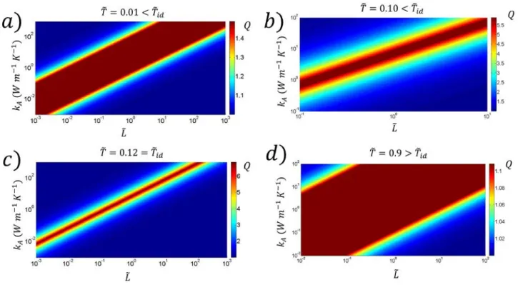
rectification performance. Figure 3a shows a piecewise volcano plot for device design at fixed 𝐿𝐿� = 1 and 𝑇𝑇� = 0.1 values, for a certain system with 𝑘𝑘𝐵𝐵,1 = 50 W m-1 K-1 and 𝑘𝑘𝐵𝐵,2 = 1 W m-1 K-1. It is apparent that a maximum in rectification is approached as the two outer regions (Case I and Case II) converge towards a mixed model region, which is characterized by a Case I model in one temperature bias and a Case II model in the other temperature bias. Furthermore, it is clear that the device will yield an optimum thermal rectification ratio when the design is such that the transition temperature occurs at the interface between the phase change material B and the invariant material A under both temperature biases. This occurs at an ideal temperature bias, where the region modeled with Case I and the region modeled with Case II converges, such that the mixed model region collapses, as can be seen in Figure 3b.
Mathematically, the convergence of the Case I and Case II regions occurs when 𝛿𝛿 = 𝐿𝐿𝐵𝐵 for both temperature biases. This is a stricter constraint than that for Case II, which was presented in Equation (26) and (27), because it indicates that the device is operating such that 𝑇𝑇𝑖𝑖 = 𝑇𝑇∗. On the other hand, Equation (26) and (27) for Case II, only require that material B exists in a single phase and that 𝑇𝑇∗ can
occur anywhere within material A. Applying this constraint to Equation (26) and (27) yields Equation (33), indicating that there is an ideal 𝑇𝑇� for device performance for a given 𝑘𝑘𝐵𝐵,1 and 𝑘𝑘𝐵𝐵,2.
𝑇𝑇�𝑖𝑖𝑑𝑑 = �𝑘𝑘𝐵𝐵,2
�𝑘𝑘𝐵𝐵,2+�𝑘𝑘𝐵𝐵,1 (33)
where 𝑇𝑇�𝑖𝑖𝑑𝑑 refers to the ideal 𝑇𝑇� for device performance.
Application of this ideal temperature bias, 𝑇𝑇�𝑖𝑖𝑑𝑑, to Equation (26) or (27) yields Equation (34), which provides the necessary relationship between 𝑘𝑘𝐴𝐴 and 𝐿𝐿� for optimum device performance. In addition, application of Equation (33) to Equation (28) yields Equation (35), which provides the maximum thermal rectification ratio that can be obtained by the system. Equation (34) and (35) is supported by recent analytical work performed by Zhang et al.[30]
𝑘𝑘𝐴𝐴 = 𝐿𝐿��𝑘𝑘𝐵𝐵,1𝑘𝑘𝐵𝐵,2 (34) 𝑄𝑄𝑚𝑚𝑚𝑚𝜕𝜕 =�𝑘𝑘𝐵𝐵,1𝑘𝑘𝐵𝐵,2+𝑘𝑘𝐵𝐵,2
�𝑘𝑘𝐵𝐵,1𝑘𝑘𝐵𝐵,2+𝑘𝑘𝐵𝐵,1 (35)
where 𝑄𝑄𝑚𝑚𝑚𝑚𝜕𝜕 refers to the maximum thermal rectification ratio that can be achieved by the system when operated at the ideal temperature bias, 𝑇𝑇�𝑖𝑖𝑑𝑑, with the system’s thermal resistances also satisfying
Equation (34).
For the model system described in Figure 3, the application of Equation (33) and (35) indicates that 𝑇𝑇�𝑖𝑖𝑑𝑑 and 𝑄𝑄𝑚𝑚𝑚𝑚𝜕𝜕 are 0.12 and 7.1, respectively. This thermal rectification will be achieved at the given 𝑇𝑇�𝑖𝑖𝑑𝑑 provided that the thermal resistances within the system satisfy Equation (34). Figure 4 shows the evolution of a contour plot for the thermal rectification ratio as 𝑇𝑇� is varied for this particular system. It is apparent that as 𝑇𝑇�𝑖𝑖𝑑𝑑 is approached from above and below, the mixed model region collapses and the
optimal rectification ratio enhances dramatically. In addition, the linear relationship between 𝑘𝑘𝐴𝐴 and 𝐿𝐿� is shown in the contour plots.
3. Application to Experimental Phase Change Materials
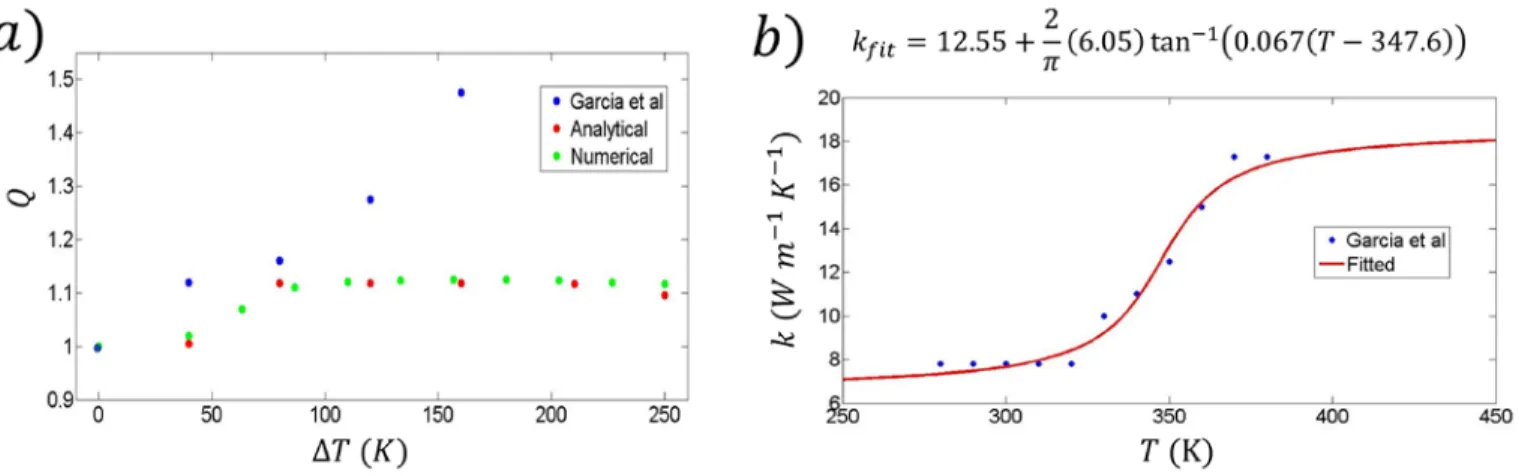
A thermal diode based on the junction between the crystalline phase change material nitinol (B) and the invariant material graphite (A) was developed by Garcia et al.[27] For this system 𝑘𝑘
𝐵𝐵,1 and 𝑘𝑘𝐵𝐵,2 would be defined by the crystal lattice structures of martensite (7.8 W m-1 K-1) and austenite (17.3 W m-1 K-1), respectively, for the nitinol phase change material (B). In addition, 𝐿𝐿� = 1 and 𝑇𝑇∗ = 330 𝐾𝐾, based on the reference data provided by Garcia et al. The invariant material (A), graphite, is assumed to have a temperature invariant thermal conductivity of 72.5 W m-1 K-1, also based on reference data provided by the researchers. For their thermal rectification measurements, the researchers maintained 𝑇𝑇1 = 290 𝐾𝐾 and varied 𝑇𝑇2 up to 450 𝐾𝐾. Based on the provided temperature boundary condition values, 𝑇𝑇� ranges can be calculated and the applicable models for certain temperature boundary conditions can be determined. Figure 5a shows a comparison of the experimental thermal rectification results from Garcia et al. with numerically and analytically derived thermal rectification ratios for the system. The numerically derived thermal rectification ratios were obtained according to the strategy outlined for Equation (32), using the thermal conductivity data provided by Garcia et al. for nitinol and graphite as functions of temperature. The thermal conductivity data provided by the researchers were fitted to a smooth function in order to numerically calculate the expected thermal rectification ratios. It should be noted that the temperature range for the experimental thermal conductivity values for nitinol reported by Garcia et al. is 280 𝐾𝐾 < 𝑇𝑇 < 380 𝐾𝐾. Therefore, when 𝑇𝑇2 = 390 𝐾𝐾 and ∆𝑇𝑇 = 100 𝐾𝐾, the range of known thermal conductivity values for nitinol has been exceeded. In order to compare experimental data with the numerical and analytical models, it was assumed that above 𝑇𝑇 = 380 𝐾𝐾 the thermal conductivity plateaued at the value for austenite. The analytical models applied to the system refer to
the Case I and Case II models, which were appropriately applied according to Table 1, depending on the applied temperature bias and the thermophysical properties of the system. The developed analytical models should only be applied to the experimental data with temperature biases enclosing the phase transition temperature. For that reason, analytically derived data points are not present as the temperature bias decreases in Figure 5a. It is apparent that the numerical and analytical calculations for the expected thermal rectification values are in agreement. In addition, the experimental thermal rectification values are in agreement with the models until ∆𝑇𝑇 = 100 𝐾𝐾 is reached. However, at temperature biases ∆𝑇𝑇 > 100 𝐾𝐾 – the range where we have extrapolated the thermal conductivity values for nitinol – the numerical and analytical models are no longer in agreement with the experimental thermal rectification values. We attribute this disagreement to the lack of experimental data for the thermal conductivity of the nitinol material above 𝑇𝑇 = 380 𝐾𝐾.
A thermal diode based on a phase change polymer has been experimentally and conceptually discussed by Pallecchi et al.[29] The thermal diode consists of a PNIPAM-PDMS two-segment system, in which PNIPAM acts as the phase change material (B) and PDMS acts as an invariant material (A). Experimental thermal rectification values are not explicitly reported by Pallecchi et al. However, values for thermal fluxes under a variety of forward and reverse temperature biases are reported, refer to Figure 6a, which can be used to calculate experimental values for the thermal rectification of their system, as shown in Figure 6b. As previously mentioned, for application of the developed analytical models, it is necessary for the temperature biases to enclose the phase transition temperature. This accounts for the range of the experimental data provided in Figure 6a. The heat flux data for the forward and reverse temperature biases were fitted with linear regressions in order to calculate the experimental thermal rectification ratio as a function of the magnitude of the temperature bias, as shown in Figure 6b. Based on the thermal resistances and system dimensions provided by the researchers, the relevant values for modeling this system are: 𝑘𝑘𝐵𝐵,1 = 0.101 W m-1 K-1, 𝑘𝑘𝐵𝐵,2 = 0.396 W
m-1 K-1, 𝑘𝑘𝐴𝐴 = 0.101 W m-1 K-1, and 𝐿𝐿� = 1. Using these system parameters, the device constructed by Pallecchi et al. can be modeled with the analytical equations that have been presented, as shown in Figure 6b. The experimental results provided by Pallecchi et al. validate the developed analytical models, as indicated by the convergence of the experimental thermal rectification ratios (black) to the maximum predicted by the analytical model (green). Furthermore, the agreement between the experimental data and the analytical model indicates the utility of this straightforward, algebraic model towards accurately predicting thermal rectification performance and towards the effective design of such thermal diodes.
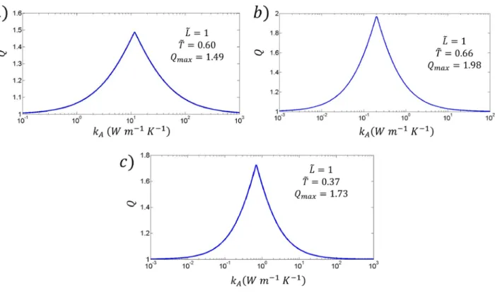
The design strategy outlined in Equation (33-35) for attaining the maximum thermal rectification can be applied to the systems described by Garcia et al. and Pallecchi et al. Application of these equations yields the optimal temperature gradient and the maximum attainable thermal rectification ratio. For operation of the devices at the ideal temperature gradient, the performance of the system can be modeled as a function of the thermal conductivity of the invariant material (A), in order to determine the ideal material to couple to the phase change material. Therefore, we will consider the phase change materials (B) employed by Garcia et al. and Pallecchi et al., but we will design for a more appropriate phase-invariant material (A), other than graphite and PDMS, respectively. Figure 7 presents the results of these simulations. It should also be noted that the length scales for the devices proposed by Garcia et
al. and Pallecchi et al. could have been adjusted according to Equation (34), instead of selecting
another phase invariant material. Properly tuning the thermal conductivities or system length scales yields maximum thermal rectification ratios of 1.49 and 1.98 for the systems described by Garcia et al. and Pallecchi et al., respectively. For the thermal diode system developed by Garcia et al., this
maximum thermal rectification ratio of 1.49 refers to the maximum thermal rectification ratio that can be attained within the window of operation constrained by the range of the experimental thermal
conductivity data – where the numerical and analytical models are in agreement with the experimental data.
The ability to tune electrical and thermal conductivity with liquid-solid phase transitions in percolated composite materials has been recently reported in literature.[31] For a system of suspended graphite flakes in hexadecane, the room temperature liquid-solid phase transition results in a step-like change in thermal conductivity. Factors of 3.2 were reported for thermal conductivity amplification. In addition, the thermal conductivity showed stable, cycling behavior. For a 1 vol% suspension of graphite flakes in hexadecane, the relevant thermal properties are: 𝑘𝑘𝐵𝐵,1 = 1.2 W m-1 K-1 and 𝑘𝑘𝐵𝐵,2 = 0.4 W m-1 K-1. The ideal temperature gradient (𝑇𝑇�) for this system is 0.37 and the maximum achievable thermal rectification ratio is 1.73. Figure 7c provides insight towards the selection of the invariant material (A) to interface with the suspension such that optimal thermal rectification performance can be achieved.
4. Conclusion
In this work we have developed an analytical model based on continuum laws of heat conduction to describe thermal rectification in devices that incorporate phase transition materials. The analytical model can be used to understand the effects of the system’s thermal resistances, as well as the applied temperature gradients, on the device’s thermal rectification performance. For a given phase transition material (B), with a certain phase transition temperature (𝑇𝑇∗), as well as characteristic thermal conductivities for each phase (𝑘𝑘𝐵𝐵,1 𝑘𝑘𝐵𝐵,2), we outline a procedure for designing a thermal rectifying device with optimal performance using this analytical model. The procedure involves properly tuning the thermal resistances of the phase change material (B) and the phase invariant material (A), in addition to properly selecting a thermal bias for operation.
The analytical model was applied to experimental data in literature for two thermal diodes, which incorporated phase change materials, developed by Garcia et al. and Pallecchi et al. The comparison
between the experimental data and the analytical predictions for the two thermal diode systems showed agreement. For the nitinol-graphite thermal diode system developed by Garcia et al., the analytical and numerical thermal rectification predictions were in agreement. Furthermore, the theoretical models, numerical and analytical, were in agreement with the experimental data reported by Garcia et al. until a temperature bias of ∆𝑇𝑇 = 100 𝐾𝐾 was reached. Temperature biases ∆𝑇𝑇 > 100 𝐾𝐾 exceeded the known range for the thermal conductivity of the nitinol material and account for the discrepancy between theory and experiment at larger temperature biases. Though thermal rectification ratios for the thermal diode system developed by Pallecchi et al. were not explicitly reported, the values were able to be calculated from reported thermal flux values as a function of temperature bias. The calculated, experimental thermal rectification ratios for the PNIPAM-PDMS thermal diode system from Pallecchi
et al. were in strong agreement with the analytical model. The analytical model was also applied to
optimize the design of the thermal diodes developed by Garcia et al. and Pallecchi et al. For the nitinol thermal diode system, in the range of known thermal conductivity, it was shown that the thermal rectification ratio could be significantly enhanced by choosing a phase invariant material to replace graphite. The same conclusion was demonstrated for the PNIPAM thermal diode system – choosing a phase invariant material to replace the PDMS could drastically increase the thermal rectification ratio. Lastly, the analytical model was applied to the optimal design of a thermal diode based on a known phase transition material, which undergoes a modulation of thermal conductivity during its phase transition. The composite material, exfoliated graphite in hexadecane, undergoes thermal conductivity modulation in response to effects on the percolation network for heat conduction due to crystallinity changes during the phase transition. The maximum thermal rectification for this system was predicted to be 1.73 by the analytical model.
Acknowledgements
The authors acknowledge the Air Force Office of Scientific Research (AFOSR), under award FA9550-09-1-0700, for their financial support regarding this project.
Received: ((will be filled in by the editorial staff)) Revised: ((will be filled in by the editorial staff)) Published online: ((will be filled in by the editorial staff)) References
[1] L. Wang, B. Li, Phys. World 2008, 21, 27. [2] C. Starr, Physics 1936, 7, 15.
[3] B. Li, L. Wang, G. Casati, Appl. Phys. Lett. 2006, 88, 143501-1.
[4] J. Zhu, K. Hippalgaonkar, S. Shen, K. Wang, Y. Abate, S. Lee, J. Wu, X. Yin, A. Majumdar, X. Zhang, Nano Lett. 2014, 14, 4867.
[5] W. C. Lo, L. Wang, B. Li, J. Phys. Soc. Japan 2008, 77, No. 5. [6] N. Yang, N. Li, L. Wang, B. Li, Phys. Rev. B 2007, 76, 020301-1. [7] L. Wang, B. Li, Phys. Rev. Lett. 2007, 99, 177208-1.
[8] L. Wang, B. Li, Phys. Rev. Lett. 2008, 101, 267203-1. [9] B. Li, J. Lan, L. Wang, Phys. Rev. Lett. 2005, 95, 104302-1. [10] N. A. Roberts, D. G. Walker, Int. J. Therm. Sci. 2011, 50, 648.
[11] V. Kislitsyn, S. Pavliuk, R. Soltys, V. Lozovski, G. Strilchuk, IEEE Trans. Electron Devices 2014, 61, 548.
[12] R. Scheibner, M. König, D. Reuter, a D. Wieck, C. Gould, H. Buhmann, L. W. Molenkamp, New
J. Phys. 2008, 10, 083016.
[13] C. W. Chang, D. Okawa, A. Majumdar, A. Zettl, Science 2006, 314, 1121. [14] P. W. O’Callaghan, S. D. Probert, a Jones, J. Phys. D. Appl. Phys. 1970, 3, 1352.
[15] D. Sawaki, W. Kobayashi, Y. Moritomo, I. Terasaki, Appl. Phys. Lett. 2011, 98, 081915. [16] M. Schmotz, J. Maier, E. Scheer, P. Leiderer, New J. Phys. 2011, 13, 113027.
[17] H. Tian, D. Xie, Y. Yang, T.-L. Ren, G. Zhang, Y.-F. Wang, C.-J. Zhou, P.-G. Peng, L.-G. Wang, L.-T. Liu, Sci. Rep. 2012, 2, 523.
[18] C. Marucha, J. Mucha, J. Rafałowicz, Phys. status solidi 1975, 31, 269. [19] A. Jeżowski, J. Rafalowicz, Phys. status solidi 1978, 47, 229.
[20] K. Balcerek, T. Tyc, Phys. status solidi 1978, 47, K125.
[21] W. Kobayashi, Y. Teraoka, I. Terasaki, Appl. Phys. Lett. 2009, 95, 171905-1.
[22] T. Takeuchi, H. Goto, Y. Toyama, T. Itoh, M. Mikami, J. Electron. Mater. 2011, 40, 1129. [23] M. Peyrard, Europhys. Lett. 2006, 76, 49.
[24] B. Hu, D. He, L. Yang, Y. Zhang, Phys. Rev. E 2006, 74, 060201-1. [25] L. Wang, B. Li, Phys. Rev. E 2011, 83, 061128-1.
[26] C. Dames, J. Heat Transfer 2009, 131, 061301-1.
[27] K. I. Garcia-Garcia, J. Alvarez-Quintana, Int. J. Therm. Sci. 2014, 81, 76. [28] P. Ben-Abdallah, S. A. Biehs, Appl. Phys. Lett. 2013, 103, 191907-1.
[29] E. Pallecchi, Z. Chen, G. E. Fernandes, Y. Wan, J. H. Kim, J. Xu, Mater. Horiz. 2015, 2, 125. [30] T. Zhang, T. Luo, Small, 2015, DOI: 10.1002/smll.201501127
[31] R. Zheng, J. Gao, J. Wang, G. Chen, Nat. Commun. 2011, 2, 289.
Figures:
Figure 1. A schematic illustrating thermal rectification in a device consisting of a phase change material (B),
with each phase characterized by a different thermal conductivity (𝑘𝑘𝐵𝐵,1, 𝑘𝑘𝐵𝐵,2), interfaced with a phase invariant material (A) with thermal conductivity 𝑘𝑘𝐴𝐴. a) A representation of the temperature profile (red line) throughout the system when the external boundary of material B is below the transition temperature (𝑇𝑇∗) and the external boundary of material A is above the transition temperature. The illustrated temperature profile is for the case
where 𝑘𝑘𝐵𝐵,1, 𝑘𝑘𝐵𝐵,2, & 𝑘𝑘𝐴𝐴 are constant with respect to temperature. b) A representation of the temperature profile (red line) throughout the system when the external boundary of material B is above the transition temperature and the external boundary of material A is below the transition temperature. The illustrated temperature profile
is for the case where 𝑘𝑘𝐵𝐵,1, 𝑘𝑘𝐵𝐵,2, 𝑎𝑎𝑎𝑎𝑎𝑎 𝑘𝑘𝐴𝐴 are constant with respect to temperature. The spatial distribution of the phases within material B as the temperature boundary conditions are reversed should be noted.
Figure 2. A schematic qualitatively illustrating thermal rectification in a device consisting of a phase change
material (B), with each phase characterized by a different thermal conductivity (𝑘𝑘𝐵𝐵,1, 𝑘𝑘𝐵𝐵,2), interfaced with a phase invariant material (A) with thermal conductivity 𝑘𝑘𝐴𝐴. a) A representation of the temperature profile (red line) throughout the system when the external boundary of material B is below the transition temperature (𝑇𝑇∗) and the external boundary of material A is above the transition temperature. The illustrated temperature profile
is for the case where 𝑘𝑘𝐵𝐵,1 & 𝑘𝑘𝐴𝐴 are constant with respect to temperature. b) A representation of the temperature profile (red line) throughout the system when the external boundary of material B is above the transition temperature and the external boundary of material A is below the transition temperature. The illustrated
temperature profile is for the case where 𝑘𝑘𝐵𝐵,2, & 𝑘𝑘𝐴𝐴 are constant with respect to temperature. The distribution of the phases within material B as the temperature boundary conditions are reversed should be noted. Also, it can
be noted that the transition temperature, 𝑇𝑇∗, occurs at a distance 𝑥𝑥 > 𝐿𝐿𝐵𝐵.
Table 1. A chart summarizing the results for the estimation of the thermal rectification ratio for a given system
consisting of a junction between an invariant material with constant thermal conductivity and a phase change material with constant thermal conductivities for each phase. 𝐴𝐴 > 𝐵𝐵 & 𝐶𝐶 > 𝐷𝐷 refers to a strictly Case I system. 𝐴𝐴 ≤ 𝐵𝐵 & 𝐶𝐶 ≤ 𝐷𝐷 refers to a strictly Case II system. The other two possibilities refer to a mixing of Case I and Case II.
Figure 3. Plots illustrating the effects of the thermal conductivity of the invariant material (A) and the applied
temperature bias towards the optimization of the thermal rectification performance for an assumed phase change
material (B). a) A plot allowing optimal design of the thermal rectification ratio, 𝑄𝑄, as a function of the thermal conductivity of the invariant material (A), 𝑘𝑘𝐴𝐴, for a fixed 𝐿𝐿� = 1 & 𝑇𝑇� = 0.1. 𝑘𝑘𝐵𝐵,1= 50 W m-1 K-1 & 𝑘𝑘
𝐵𝐵,2= 1 W
m-1 K-1 are also fixed as properties of the phase change material that is assumed. The plot is a piecewise
function, where the relevant models used to derive specific regions are indicated by brackets. b) A contour plot demonstrating the convergence of Case I and Case II and the collapse of the mixed model region, yielding an
optimal thermal rectification performance, as an ideal temperature bias is approached. 𝑄𝑄 is plotted as a function of the thermal conductivity of the invariant material (A), 𝑘𝑘𝐴𝐴, and the applied temperature bias, 𝑇𝑇� at fixed 𝐿𝐿� = 1. Again, 𝑘𝑘𝐵𝐵,1= 50 W m-1 K-1 & 𝑘𝑘
𝐵𝐵,2= 1 W m-1 K-1 are also fixed as properties of the phase change material that
is assumed.
Figure 4. For a model system with 𝑘𝑘𝐵𝐵,1 = 50 W m-1 K-1 & 𝑘𝑘
𝐵𝐵,2= 1 W m-1 K-1, the evolution of a contour plot
for the thermal rectification ratio, 𝑄𝑄, as a function of 𝐿𝐿� and 𝑘𝑘𝐴𝐴 (W m-1 K-1), as 𝑇𝑇� is varied around 𝑇𝑇�
𝑖𝑖𝑑𝑑 is shown. a)
Contour plot for 𝑇𝑇� = 0.01. b) Contour plot for 𝑇𝑇� = 0.10. c) Contour plot for 𝑇𝑇� = 𝑇𝑇�𝑖𝑖𝑑𝑑= 0.12. d) Contour plot for 𝑇𝑇� = 0.9.
Figure 5. Comparison of the experimental thermal rectification ratios obtained by Garcia et al. for their nitinol
phase change-based thermal diode to analytically and numerically predicted thermal rectification ratios for the system.[27]. The analytically calculated ratios were determined using the Case I and Case II models proposed
above, while the numerically calculated ratios were determined using the strategy developed by M. Peyrard as in Equation (32).[23] a) Experimental (blue), analytical (red), and numerical (green) comparison for thermal
rectification ratios as a function of temperature bias. b) A smooth function (red) fitted to the experimental thermal conductivity data (blue) from Garcia et al. for nitinol as a function of temperature.
Figure 6. A comparison of the experimental thermal rectification data from Pallecchi et al. with the analytical
thermal rectification predictions from the Case I and Case II models.[29] a) A plot of the heat flow, 𝑞𝑞, measured
by Pallecchi et al. for their phase change-based thermal diode under a range of forward (orange) and reverse
(blue) temperature biases, ∆𝑇𝑇.[29] The data for each temperature bias were fitted with a linear regression. b) A
plot of the experimental and analytically predicted thermal rectification ratios, 𝑄𝑄, as a function of the applied temperature bias, ∆𝑇𝑇, for the phase change-based thermal diode developed by Pallecchi et al.[29] The
experimental thermal rectification data (black), obtained from a ratio of the linear fits in a), is compared with the analytically predicted thermal rectification data (green). This diode incorporated a PNIPAM polymer as the phase change material (B) and a PDMS polymer as the phase invariant material (A). The relevant
thermophysical parameters reported by the researchers, and used to model the system, are reported within the figure. The analytical thermal rectification values were generated according to the strategy outlined in Table 1, and they show significant agreement with the experimental values.
Figure 7. Optimization design plots for two phase change-based thermal diodes discussed in literature and an
additional phase change material with thermal conductivity modulation that has yet to be incorporated into a thermal diode. a) Design plot for the nitinol-based thermal diode developed by Garcia et al.[27] The thermal
rectification ratio, 𝑄𝑄, as a function of the thermal conductivity, 𝑘𝑘𝐴𝐴, of the invariant material (A) is plotted for 𝑇𝑇� = 𝑇𝑇�𝑖𝑖𝑑𝑑 = 0.60 and 𝐿𝐿� = 1. b) Design plot for the PNIPAM-based thermal diode developed by Pallecchi et al.[29]
The thermal rectification ratio, 𝑄𝑄, as a function of the thermal conductivity, 𝑘𝑘𝐴𝐴, of the invariant material (A) is 27
plotted for 𝑇𝑇� = 𝑇𝑇�𝑖𝑖𝑑𝑑 = 0.66 and 𝐿𝐿� = 1. c) Design plot for a thermal diode based on liquid-solid phase transitions in a suspension of graphite flakes in hexadecane.[31] The thermal rectification ratio, 𝑄𝑄, as a function of the
thermal conductivity, 𝑘𝑘𝐴𝐴, of the invariant material (A) is plotted for 𝑇𝑇� = 𝑇𝑇�𝑖𝑖𝑑𝑑 = 0.37 and 𝐿𝐿� = 1.
Table of Contents:
Phase change materials can be used to construct thermal diodes. It is shown mathematically that the interface of such materials with a phase invariant material can function as a thermal diode. Criteria are derived analytically for the choice of thermal conductivity of the invariant phase to maximize the thermal rectification, and the model is applied to experimental systems in the literature.
Keyword: thermal diodes
Anton L. Cottrill, Michael S. Strano*
Analysis of Thermal Diodes Enabled by Junctions of Phase Change Materials