Evaluation of the ORCHIDEE ecosystem model over Africa against 25 years of satellite-based water and carbon measurements

HAL Id: hal-02927856

https://hal.archives-ouvertes.fr/hal-02927856

Submitted on 17 Sep 2020

HAL is a multi-disciplinary open access

archive for the deposit and dissemination of

sci-entific research documents, whether they are

pub-lished or not. The documents may come from

teaching and research institutions in France or

abroad, or from public or private research centers.

L’archive ouverte pluridisciplinaire HAL, est

destinée au dépôt et à la diffusion de documents

scientifiques de niveau recherche, publiés ou non,

émanant des établissements d’enseignement et de

recherche français ou étrangers, des laboratoires

publics ou privés.

Africa against 25 years of satellite-based water and

carbon measurements

Abdoul Khadre Traore, Philippe Ciais, Nicolas Vuichard, Benjamin Poulter,

Nicolas Viovy, Matthieu Guimberteau, Martin Jung, Ranga Myneni, Joshua

Fisher

To cite this version:

Abdoul Khadre Traore, Philippe Ciais, Nicolas Vuichard, Benjamin Poulter, Nicolas Viovy, et al..

Evaluation of the ORCHIDEE ecosystem model over Africa against 25 years of satellite-based water

and carbon measurements. Journal of Geophysical Research: Biogeosciences, American Geophysical

Union, 2014, 119 (8), pp.1554-1575. �10.1002/2014JG002638�. �hal-02927856�

Evaluation of the ORCHIDEE ecosystem model

over Africa against 25 years of satellite-based

water and carbon measurements

Abdoul Khadre Traore1, Philippe Ciais1, Nicolas Vuichard1, Benjamin Poulter2, Nicolas Viovy1, Matthieu Guimberteau3, Martin Jung4, Ranga Myneni5, and Joshua B. Fisher6

1

Laboratoire des Sciences du Climat et de l’Environnement, LSCE/IPSL - CEA-CNRS-UVQS, Gif sur Yvette, France, 2_{Department of Ecology, Montana State University, Bozeman, Montana, USA,}3_{Institut Pierre Simon Lapalce, Paris, France,} 4

Max Planck Institute for Biogeochemistry, Jena, Germany,5Department of Earth and Environment, Boston University, Boston, Massachusetts, USA,6_{Department of Environmental Science, Policy, and Management, University of California at} Berkeley, Berkeley, California, USA

Abstract

Few studies have evaluated land surface models for African ecosystems. Here we evaluate the Organizing Carbon and Hydrology in Dynamic Ecosystems (ORCHIDEE) process-based model for the interannual variability (IAV) of the fraction of absorbed active radiation, the gross primary productivity (GPP), soil moisture, and evapotranspiration (ET). Two ORCHIDEE versions are tested, which differ by their soil hydrology parameterization, one with a two-layer simple bucket and the other a more complex 11-layer soil-water diffusion. In addition, we evaluate the sensitivity of climate forcing data, atmospheric CO₂, and soil depth. Beside a very generic vegetation parameterization, ORCHIDEE simulates rather well the IAV of GPP and ET (0.5< r < 0.9 interannual correlation) over Africa except in forestlands. The ORCHIDEE 11-layer version outperforms the two-layer version for simulating IAV of soil moisture, whereas both versions have similar performance of GPP and ET. Effects of CO₂trends, and of variable soil depth on the IAV of GPP, ET, and soil moisture are small, although these drivers influence the trends of these variables. The meteorological forcing data appear to be quite important for faithfully reproducing the IAV of simulated variables, suggesting that in regions with sparse weather station data, the model uncertainty is strongly related to uncertain meteorological forcing. Simulated variables are positively and strongly correlated with precipitation but negatively and weakly correlated with temperature and solar radiation. Model-derived and observation-based sensitivities are in agreement for the driving role of precipitation. However, the modeled GPP is too sensitive to precipitation, suggesting that processes such as increased water use efficiency during drought need to be incorporated in ORCHIDEE.

1. Introduction

Africa has experienced overall high climate variability over the course of the twentieth century and particularly in the last three tofive decades [Ackerley et al., 2011; Biasutti, 2013; Funk et al., 2008; Hession and Moore, 2011; Hoerling et al., 2006; Lebel and Ali, 2009; Mohamed, 2011; New et al., 2006; Rosell and Holmer, 2007; Williams and Funk, 2011]. This high climate variability, particularly at an interannual scale, makes the continent vulnerable by affecting terrestrial ecosystem productivity, particularly though carbon and water cycling between vegetation, soils, and atmosphere. Yet in spite of regional vulnerabilities to climate variability and uncertainties in future responses to regional climate change [Solomon, 2007], the recent variability of African productivity and waterfluxes in response to climate, rising atmospheric dioxide carbon (CO2), and increased

human pressure, remains poorly studied. The largest uncertainties in African productivity stem from the response to increasing CO2as well as climate extremes [Fisher et al., 2013]. To reduce uncertainties on projected

future changes of productivity and their linkage with water availability, it is important for ecosystem models to faithfully reproduce, the present-day dynamics, including interannual variability (IAV), of gross primary productivity (GPP) and waterfluxes, both for natural and managed ecosystems.

This study aims to assess the IAV of (1) Africa’s vegetation cover (through the fraction of absorbed

photosynthetically active radiation (fAPAR)), (2) productivity (GPP), (3) waterfluxes (through evapotranspiration (ET)), and (4) soil moisture over the last three decades simulated by different versions of the ORCHIDEE (Organizing Carbon and Hydrology in Dynamic Ecosystems) process-based land surface model. The model

Journal of Geophysical Research: Biogeosciences

RESEARCH ARTICLE

10.1002/2014JG002638

Special Section:

Experiment-Model Integration in Terrestrial Ecosystem Study: Current Practices and Future Challenges

Key Points:

• High sensitivity of grassland fluxes to climate compared to closed forests • CO2and variable soil depth are small

effect on the IAV of GPP and ET • Relationship between carbon flux

IAV and T2m temperature is weak and negative Supporting Information: • Figure S1 • Figure S2 • Figure S3 • Figure S4 • Figure S5 Correspondence to: A. K. Traore, traore@lsce.ipsl.fr Citation:

Traore, A. K., P. Ciais, N. Vuichard, B. Poulter, N. Viovy, M. Guimberteau, M. Jung, R. Myneni, and J. B. Fisher (2014), Evaluation of the ORCHIDEE ecosystem model over Africa against 25 years of satellite-based water and carbon measurements, J. Geophys. Res. Biogeosci., 119, 1554–1575, doi:10.1002/ 2014JG002638.

Received 4 FEB 2014 Accepted 13 JUL 2014

Accepted article online 17 JUL 2014 Published online 14 AUG 2014

evaluation is performed using satellite data, which are valuable in a context of scarce in situ data in Africa [Ciais et al., 2011]. Satellite products were used to estimate phenology and carbonfluxes over Africa in several previous studies [Jung et al., 2009; Owe et al., 2008; Weber et al., 2008; Yuan et al., 2011]. The level of confidence in the ecosystem models for Africa remains low as they are generally not calibrated against regional

measurements and may poorly represent specific processes, such as phenology and soil hydrology, as well as water efficiency. Moreover, a source of uncertainty in land surface model output also comes from uncertain climate input data [Poulter et al., 2011], in particular, over Africa where there has been attrition of meteorological networks. To estimate the bias in model output caused by the choice of a climate forcing data set, we have run ORCHIDEE with two different gridded climate forcing data Watch Forcing Data - EraInterim (WFDEI) and Watch Forcing Data (WFD) [Weedon et al., 2010, 2011] from the same WATer and global CHange project (WATCH) project.

In this study, we combine measurements and model simulations to address the following questions:

1. Is the performance of the 11-layer soil hydrology ORCHIDEE version superior to the simpler two-layer scheme, for simulating the average spatial distribution of fAPAR, GPP, ET, and soil moisture within African regions when compared with the evaluation data sets?

2. What are the ecoclimatic regions of Africa that have the largest IAV, and do the model simulations capture them?

3. Is the performance of the 11-layer soil hydrology superior for simulating IAV of fAPAR, GPP, ET, and soil moisture, as well as the average difference of these variables between wet and dry years, over different African regions?

4. What is the effect of the choice of a meteorological forcing data on the model-data misfit for the IAV of fAPAR, GPP, ET, and soil moisture?

5. What are the climatic drivers (temperature, precipitation, and radiation) of the IAV of fAPAR, GPP, ET, and soil moisture, and the sensitivity offluxes to these drivers?

6. Did rising CO2over the past three decades influence the IAV of modeled fAPAR, GPP, ET, and soil moisture?

Did soil depth (uniformlyfixed or variable within vegetation) influence the IAV of these variables? In the following sections, wefirst present a description of the different versions and configurations of the ORCHIDEE model (section 2) and describe the climate forcing data as well the simulations used in this study (section 3) and the satellite data sets used for evaluation in section 4. In section 5.1, we show the capability of ORCHIDEE to simulate the spatial pattern of average fAPAR, GPP, ET, and soil moisture and analyze their IAV in section 5.2. The contrast between composite wet and dry years (absolute difference between the average of all wet years and the average of all dry years since 1979) is further examined in section 5.3. Finally, in section 5.4, we investigate the relationship between fAPAR, GPP, ET, soil moisture, and climate drivers, before drawing conclusions in section 6.

2. ORCHIDEE Model Parameterizations

ORCHIDEE is a land surface model that simulates carbon, water, and energy exchanges within ecosystems and between the land and the atmosphere [Krinner et al., 2005]. The land vegetation is discretized using 12 plant functional types (PFTs) and bare soil. The definition of a PFT is deduced from a tree classification that accounts for physiognomy (tree or grass), leaf types (needleleaf or broadleaf ), phenology (evergreen, summer-green, or rain-green), the photosynthetic pathway for crops and grasses (C3 and C4), and the climatic regions (boreal, temperate, and tropical). The exchanges of energy (transfer of radiation and heat) and water balance between the vegetation-soil-atmosphere are calculated using Ducoudré et al. [1993] and De Rosnay and Polcher [1998] at a half-hourly time step. We only describe below the parameterizations of ORCHIDEE for phenology, carbon assimilation, ET, and soil moisture, which are most relevant for this study.

2.1. Carbon Processes and GPP

In ORCHIDEE, GPP represents CO2assimilation by photosynthesis and is calculated every 30 min from the

Farquhar et al. [1980] and Collatz et al. [1992] leaf-scale equations for C3 and C4 PFTs, respectively. The scaling of GPP within the canopy assumes an exponential attenuation of light, in a big-leaf approximation. Other carbonflux components such as net primary productivity, plant growth and maintenance respiration, mortality, litter, and soil organic decomposition are calculated on a daily time step following GPP. State

variables such as the leaf area index (LAI) and plant water stress from soil moisture in the root zone are prognostic and feedback on GPP, allocation, leaf age, and senescence [Krinner et al., 2005].

The description of phenology is taken from Krinner et al. [2005]. The leaf onset parameterization is based on Botta et al. [2000] with an applied criterion depending on the PFT under consideration. Over Africa, the growing season of the tropical broad-leaved rain-green trees PFT starts after a dry season and when a minimum threshold of simulated soil moisture is reached. In regions where annual mean temperature is higher than 20°C, the model has to decide regularly whether the grass leaf onset has to occur considering heat and/or moisture stress criteria according to meteorological conditions. In regions where annual temperature is between 10 and 20°C, the grass will use its carbohydrate reserve (accumulated during the previous season) to grow a minimum quantity of leaves and roots corresponding to its growing season. If the carbohydrate reserve is empty, leaf onset cannot occur, and the PFT will be removed from the grid cell. The senescence criteria are depending on temperature, water stress, and the leaf age [Krinner et al., 2005]. The plant dormancy occurs when the LAI falls below 0.2 during senescence (all the remaining leaves been shed) and a new phenological cycle can restart. Several phenological cycles can theoretically occur in 1 year for a suitable climate, e.g., with two wet seasons. In this version of ORCHIDEE, phenology of agricultural C3/C4 is treated as grass C3/C4 with adapted maximum possible LAI and slightly modified critical temperature and humidity parameters for phenology.

Water exchange through transpiration is related to photosynthesis by stomatal conductance, following the formulation of Ball et al. [1987]. The long-term processes describing vegetation dynamics,fire, and tree mortality can be either calculated (yearly time step) or prescribed in the ORCHIDEE model. In this study, vegetation dynamic was not activated butfires are accounted for. In order to account for human pressure driving the expansion of agriculture over Africa, we prescribed each year a new map of PFT distributions obtained from global land cover maps (section 3).

2.2. ET

ET is computed from potential evaporation, which depends on the humidity gradient between air and air at saturation for soil temperature [Budyko, 1961]. Potential evaporation is limited by the sum of the

aerodynamic resistance, stomatal resistance, and architectural resistance. Total ET is the sum offive components including evaporation of water intercepted by the cover, transpiration of vegetation, and bare soil evaporation. To simplify the transpiration parameterization, as well as for photosynthesis and light competition, the ORCHIDEE model does not account forfluxes from and competition with understory vegetation [Krinner et al., 2005]. Bare soil evaporation and transpiration are controlled by soil moisture and thus depend on soil hydrology parameterization in ORCHIDEE. In addition, transpiration of the cover is governed by the ability of the roots to extract water from the soil. Roots are represented in the model by an exponential root profile [De Rosnay and Polcher, 1998]. Simulated water stress from soil moisture availability influences photosynthesis and stomatal conductance through a scaling factor related to soil moisture when root zone soil moisture falls below a threshold value [McMurtrie et al., 1990]. The chosen threshold is a root extractible water (in the root zone) of 0.4, identical for all PFTs.

2.3. Soil Hydrology Processes and Soil Moisture

In this study we compare two versions of ORCHIDEE, which differs by their soil hydrology parameterizations: one version with a two-layer bucket scheme [Ducoudré et al., 1993] and one with an 11-layer soil diffusion model [D’Orgeval, 2006; De Rosnay et al., 2002; Campoy et al., Influence of soil bottom hydrological conditions on land surfacefluxes and climate in a general circulation model, submitted to Journal of Geophysical Research: Atmospheres, 2013].

The two-layer hydrology scheme is based on a simple two-layer bucket-type mode. The soil upper layer varies according to the water availability, and the deep soil layer isfilled from top to bottom with the rain. When ET is larger than precipitation, water is removed from the upper layer until it dries out, leaving only one deep soil layer. Bare soil evaporation is computed through a resistance, proportional to the relative dryness of the upper soil layer. Runoff occurs when the soil is saturated; canopy transpiration stops when the simulated soil is completely dry. The 11-layer soil scheme represents the vertical soilflow based on physical processes of nonsaturated condition from the one-dimensional Fokker-Planck equation by combining the mass and momentum conservation equations using volumetric water content [De Rosnay et al., 2002; Campoy et al., submitted manuscript, 2013]. This soil model has a multilayer discretization and equations based on the Center for

Water Resources Research model [Bruen, 1997; Dooge et al., 1993]. The vertical discretization is not uniform: the grid beingfiner near the surface (the three topmost layers being 1 cm apart) where the soil moisture mostly varies, in order to ensure that rapid exchanges of soil moisture near the surface can be represented [De Rosnay et al., 2002]. De Rosnay et al. [2000] showed that the 11-layer scheme was a suitable compromise between a detailed vertical resolution and numerical stability of calculatedfluxes. Soil texture heterogeneity between grid cells is taken into account by employing three different soil types (coarse, medium, andfine textured). The calculation of water vertical diffusion in the soil column is based on the Mualem-Van Genuchten model [Mualem, 1976; Van Genuchten, 1980], using parameters estimated by Carsel and Parrish [1988] for the corresponding soil texture classes of the United States Department of Agriculture. The soil depth of the 11-layer module isfixed at a value of 2 m everywhere. The bottom boundary condition is set to be a free drainage and the upper boundary condition driven by the soil moisture at the surface and also the meteorological variables. Bare soil evaporation is the maximum upward hydrologicalflux permitted by diffusion if thisflux is inferior to the potential evaporation. Surface runoff is governed by the precipitation rate and the capacity of the soil to infiltrate [D’Orgeval et al., 2008].

3. Model Input Data and Simulation Setup

3.1. Climate Forcing Data Sets

Two different daily climate forcing data sets, WFD and WFDEI [Weedon et al., 2010, 2011], were used in this study to drive ORCHIDEE. WFD is the WATCH Forcing Data twentieth century based on ERA40 (1958–2001) extended back to 1901 following the methodology of Weedon et al. [2010]. Since WFD stops in 2001, we extended this forcing by using the ERA-Interim data during 2001–2009. The alternative climate forcing is WFDEI, which was produced using the WFD methodology but applied to ERA-Interim reanalysis [Dee et al., 2011] with a bias correction of precipitation using (Global Precipitation Climatology Centre) GPCCv5 rain gauge measurements [Schneider et al., 2014]. The WFDEI forcing covers the period 1979–2009. Eight meteorological variables at daily time scale and at 0.5° spatial resolution are used to drive ORCHIDEE: rainfall (mm d 1), solar and infrared incoming radiation (W m 2), minimum and maximum near-surface air temperature (K), wind speed (m s 1), surface air pressure (hPa), and specific humidity (kg kg 1). These daily fields are extrapolated into half-hourly variables needed for the ORCHIDEE model. Hourly temperature was calculated over the course of the day using a sinusoidal function, rainfall was split into rain and snow (for temperature< 0°C) on each model time step. The WFDEI forcing, obtained from the more recent ERA-Interim reanalysis product compared to ERA-40 for WFD, and further corrected using precipitation measurements should be more realistic than WFD and hence give better performances.

3.2. Soil Depth and Vegetation Distribution

The natural vegetation distribution is derived from the International Geosphere Biosphere Programme map based on the Olson classification [De Rosnay and Polcher, 1998]. The transient historical crop and pasture data sets are based on the Intergovernmental Panel on Climate Change/Fifth Assessment Report (IPCC AR5) Representative Concentration Pathways simulations protocol. The historical fractions of crop and pasture are based on the History Database of the Global Environment (HYDE 3.0) database [Klein Goldewijk et al., 2011]. The variable soil depth map within vegetation profile is prescribed to the ORCHIDEE two-layer simulations only from the Harmonized World Soil Database developed by the Land Use Change and Agriculture Program of International Institute for Applied Systems Analysis (IIASA) and the Food and Agriculture Organization (FAO) for Global Agro-ecological Assessment study (GAEZ 2008). Except over the Sahara desert and some parts of northern Africa, more than 75% of grid cells have soil depth between 1.5 and 2 m (the other grid cells have less than 1.5 m of soil depth). Note that the 11-layer version is always run with afixed soil depth of 2 m.

3.3. Simulation Setup

Wefirst perform a steady state spin-up run of ORCHIDEE using the Lardy et al. [2011] method integrated into ORCHIDEE to accelerate the convergence of the soil carbon pools. Spin-up of 300 years was required to reach equilibrium in carbon pools over Africa. The spin-up run recycles climate forcing data of the 1979–1988 period at 0.5° spatial resolution with atmospheric CO₂concentrationfixed at the 1979 value (336.5 ppm). We then carried out a set of transient simulations from 1979 to 2009 starting from the end of the spin-up state. The changes of GPP and waterfluxes in response to climate and CO2are investigated usingfive factorial simulations summarized

in Table 1. Simulation S1 uses the 11-layer soil scheme with afixed 2 m soil depth and WFDEI climate with variable atmospheric CO₂and land use change. This run is expected to be the most realistic one. Simulation S2 uses the simpler two-layer soil scheme and is otherwise identical to S1. In order to analyze the effect of variable soil depth, we carried out S2-VARDEP (variable soil depth simulation), a sensitivity simulation with the two-layer scheme and a spatially variable soil depth instead of uniformlyfixed at 2 m. The effects of increasing CO2are

analyzed with the S2-FIXCO2 (simulation withfixed atmospheric CO2) simulation, identical to S2 except forfixed

atmospheric CO2concentration at the 1979 level (336.5 ppm). The sensitivity of the ORCHIDEE results to the input

climate forcing data is investigated by comparing S2-WFD driven by WFD and S2 driven by WFDEI.

3.4. Regional Partitioning of African Ecosystems

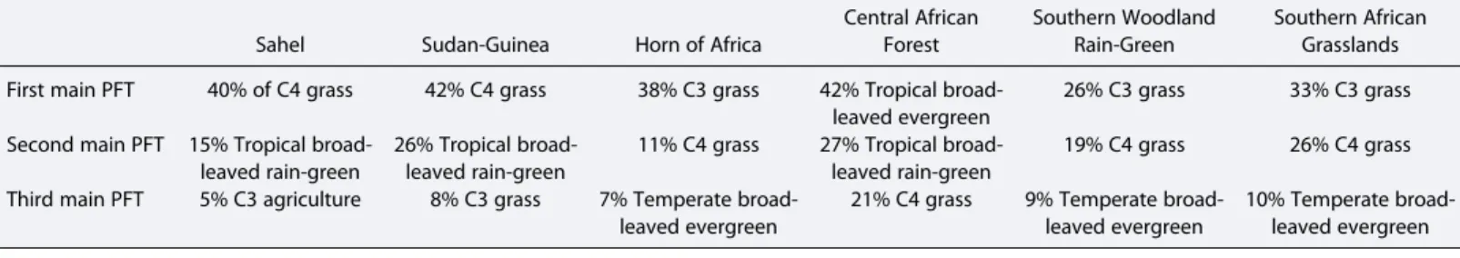
Analyses are portioned over six subregions (see Figure S1 in the supporting information for their location), defined from the distribution of African ecoclimatic-system types by Weber et al. [2008]. The northern savannah region of Weber et al. [2008] is further split into two subregions: the Sahel region (1227 grid points) representing the transition zone between the desert and the humid Guinea band zone (from 17°W to 40°E and from 12°N to 18°N) and the Sudan-Guinea region (1612 grid points): extending from 15°W to 35°E and from 5°N to 12°N. The other four regions are the central African forests (1008 grid points), the Horn of Africa (382 grid points), the southern woodland rain-green (1574 grid points) and the southern African grasslands (925 grid points). The characteristics of the seasonal cycle of the main meteorologicalfields for each ecoclimatic region are shown in Figure S1 in the supporting information and the dominant PFTs and climate data of the six subregions in Table 2. It can be seen that none of the region has a land cover for agriculture higher than 5%, the largest agricultural fraction being found in the Sahel region.

4. Data Sets for Model Evaluation

4.1. fAPAR

The latest version of the Global Inventory Modeling and Mapping System (fAPAR3g) product is used to evaluate the modeled fAPAR. This data set is available from July 1981 to December 2010. The fAPAR3g is based on the normalized difference vegetation index (NDVI)3g data [Zhu et al., 2013], which is derived from the advanced very high resolution radiometers aboard a series of satellites of National Oceanic and Atmospheric

Administration. The data set resolution is 8 km and 15 days time step. The 8 km original fAPAR3g data were reaggregated at the ORCHIDEE resolution of 0.5° using bilinear interpolation. ORCHIDEE calculates LAI each day for each PFT, and fAPAR is calculated from LAI by using the equation fAPAR = 0.95 (1 exp( 0.5 × LAI)) from Ruimy et al. [1999]. Thus, the interannual variability of modeled fAPAR has the same phase than that of LAI.

4.2. GPP and ET

We use the gridded GPP and ET data-driven model results from Jung et al. [2011]. The data-driven model is an integration of site-levelflux tower measurements of GPP and ET fluxes to the global scale using a model tree

Table 1. Overview of the ORCHIDEE Simulations Analyzed in This Study

Experiment Model Version Transient CO2 Climate Forcing Soil Depth

S1 11-layer Yes WFDEI 2 m (uniform)

S2 two-layer Yes WFDEI 2 m (uniform)

S2-FIXCO2 two-layer 336.525 ppm WFDEI 2 m (uniform)

S2-VARDEP two-layer Yes WFDEI Variable (FAO)

S2-WFD two-layer Yes WFD 2 m (uniform)

Table 2. Proportion (%) of the Three Dominant Plant Functional Types (PFTs) Within Each African Eco-climatic Sub-region Considered in This Study

Sahel Sudan-Guinea Horn of Africa

Central African Forest Southern Woodland Rain-Green Southern African Grasslands

First main PFT 40% of C4 grass 42% C4 grass 38% C3 grass 42% Tropical

broad-leaved evergreen

26% C3 grass 33% C3 grass

Second main PFT 15% Tropical broad-leaved rain-green

26% Tropical broad-leaved rain-green

11% C4 grass 27% Tropical

broad-leaved rain-green

19% C4 grass 26% C4 grass

Third main PFT 5% C3 agriculture 8% C3 grass 7% Temperate

broad-leaved evergreen

21% C4 grass 9% Temperate

broad-leaved evergreen

10% Temperate broad-leaved evergreen

ensembles (MTE) statistical model. The MTE approach is based on a combination of the Tree Induction Algorithm and the Evolving Trees with Random Growth technique described in Jung et al. [2009]. Jung et al. [2011] used the trained MTE at site level to generate global GPP (MTE-GPP) and ETfluxes (MTE-ET). The estimation of MTE-GPP and MTE-ET from extrapolation of local carbon, water, and energyfluxes eddy covariance measurements (FLUXNET) measurements is based on 29 explanatory variables, including land use, precipitation and temperature (both measured in situ), and remote sensing indices of monthly fAPAR from GIMMS during the 1982–1997 period, Sea-viewing Wide Field-of-view Sensor during 1998–2005, and Medium-Resolution Imaging Spectrometer since 2006 [Jung et al., 2011]. MTE-GPP and MTE-ET are provided at a 0.5° spatial and monthly resolution from 1982 to 2010. Cross validation of MTE-GPP and MTE-ET at site level suggested a 10% random error [Jung et al., 2010, 2011]. Note that the performance of MTE based on cross validation was found better for energyfluxes than for GPP [Jung et al., 2011]. Even though the MTE products are model results and not direct observations, they are assumed to be more realistic than the ORCHIDEE results, and hence usable for its evaluation. MTE-GPP and MTE-ET are used in this study to assess the IAV of GPP and ET. Note that virtually noflux tower measurements over the African continent were available to train the MTE, which implies a lower confidence on this product over Africa. Further, MTE-GPP and MTE-ET are not independent from the GIMMS NDVI and fAPAR, since thesefields are used to integrate flux tower measurements in space and back in time beyond theflux tower era (most of flux tower sites started only in the 2000s).

4.3. Surface Soil Moisture

The SM-MW product was developed through the European Space Agency Climate Change Initiative by Vienna University of Technology and Vrije Universiteit Amsterdam [Liu et al., 2012; Wagner et al., 2012]. The theoretical and algorithmic bases of the Soil Moisture from MicroWave (SM-MW) product are described in Owe et al. [2008]. The SM-MW is available at a resolution of 25 km daily, from 1978 to 2010. The data were reaggregated at 0.5° to match the ORCHIDEE spatial resolution used in this study. SM-MW corresponds to water present in the top 1 to 1.5 cm of the soil [Owe et al., 2008]. Retrieval of SM-MW is impossible over dense vegetation canopies, and data from central African forests are thus excluded. In ORCHIDEE, soil moisture simulated by the 11-layer soil scheme version is sampled over thefirst centimeter of soil. Soil moisture simulated by the two-layer scheme version represents the entire soil depth content (sum of moisture in the superficial layer and in the deep layer) and was compared directly with SM-MW; see also Rebel et al. [2012] for evaluation of ORCHIDEE two-layer version, against soil moisture data.

5. Model Evaluation

To harmonize the observation periods (1978–2010 for SM-MW and 1982–2010 for fAPAR3g and MTE products) with the simulations period (1979–2009), we evaluate the ORCHIDEE results over the period 1985–2009. Starting evaluation from 1985 is motivated by the need to lower the influence of the spin-up period (1979–1988, which corresponds to a dry decade especially over West Africa [Biasutti and Giannini, 2006]) on ORCHIDEE results.

5.1. Spatial Patterns

The spatial patterns of 1985–2009 average fAPAR, GPP, ET, and soil moisture (Figures 1a to 1d) from the five simulations are compared with different data products over the six African subregions using Taylor diagrams [Taylor, 2001]. The comparison between model and observation is quantified by their correlation (here spatial correlation), root-mean-square difference, and magnitude of their variations (here spatial gradients) represented by the ratios of modeled to observed standard deviation across the grid cells of each subregion.

5.1.1. fAPAR

Simulated fAPAR spatial patterns compare to the fAPAR3g observations well (Figure 1a) with positive spatial correlations r> 0.8 (at 95% confidence interval) for all simulations at the continental scale. Over subregions, highest r values are systematically found for the southern African grasslands region. In spite of a more realistic representation of soil hydrology, the 11-layer version results have a poorer spatial correlation with the fAPAR3g observations (r≈ 0.56, at 90% confidence interval). In fact, fAPAR from the two-layer simulations show better spatial correlations than with the 11-layer version over the Sahel, Sudan-Guinean, and the Horn of Africa regions (0.78< r < 0.9 at 95% confidence interval for the two-layer, compared with 0.5 < r < 0.7 at 90% confidence interval for the 11-layer version).

The choice of WFD climate forcing and the setting of variable soil depth have only a weak effect on the model performances for the fAPAR spatial patterns. In contrast with the rather high spatial correlations between modeled and observed fAPAR, all simulations give poorer performance for fAPAR spatial standard deviations (SD). This means that, despite capturing the patterns of fAPAR within each subregion, the model does not represent the magnitude of the observed spatial fAPAR gradients well. Over the southern African grasslands region, the modeled-to-observed ratio of the fAPAR SD is 2.3 in the two-layer version, and 1.2 in the 11-layer one. The two-layer version shows more realistic SD over the Sudan-Guinean band, southern woodland rain-green, and the Horn of Africa regions (SD≈ 1.3 times of fAPAR3g SD). Note also the smaller than observed fAPAR spatial standard deviation of the 11-layer version over the Sahel and the Horn of Africa regions (SD< 0.6 of fAPAR3g SD) while SD is high over the southern woodland rain-green (2.3 times of that fAPAR3g SD).

Figure 1. Taylor diagram: statistical comparison of the spatial pattern between simulations and data products (variables are averaged over the 1985–2009 period) over the six African subregions. Data products are represented by the star symbol. The axes represent the standard deviation of each variable normalized by the one of the data product. Contours represent the RMS error normalized by the data product. (a) The comparison between modeled fAPAR and fAPAR3g, (b) the modeled GPP versus MTE-GPP product, (c) the comparison between modeled ET and MTE-ET product, and (d) the modeled soil moisture versus SM-MW satellite product.

5.1.2. Gross Primary Productivity

Evaluation of spatial patterns of simulated 1985–2009 average GPP with MTE-GPP product (Figure 1b) gives similar results than for fAPAR. The two-layer version performance for the GPP spatial correlations is better than the 11-layer version, especially over the Sahel and the southern African grasslands (r≈ 0.75 at 95% confidence interval spatial correlation between two-layer GPP and MTE-GPP compared to r < 0.5 in the 11-layer version). In contrast, all simulations show low spatial correlations of modeled GPP with MTE-GPP over the central African forest and the southern woodland rain-green regions (0.1< r < 0.5). This suggests that either the MTE-GPP gradients, calculated from satellite fAPAR and climate predictors, are not very reliable due, for example, to the presence of clouds over forests or that climate is not the main driver of GPP gradients in those two regions. The spatial standard deviations of ORCHIDEE GPP are systematically too high in comparison with MTE-GPP (Figure 1b). However, the 11-layer version has a very low SD over the Sahel and the Horn of African regions (SD< 0.6 times of that MTE-GPP SD). Like for fAPAR, the choice of WFD climate forcing compared to WFDEI has a very small effect on the model performance for spatial patterns of GPP.

5.1.3. Evapotranspiration

By contrast with GPP and fAPAR, modeled ET (Figure 1c) shows better performance for both ORCHIDEE versions over all African subregions and especially over the southern African grasslands and Sahel regions. We found in these regions a correlation of r≈ 0.8 at 95% confidence interval between the 11-layer version and the MTE-ET (r≈ 0.9 at 95% confidence interval for the two-layer version) and SD ≈ 0.8 of MTE-ET SD (SD≈ 1.01 of MTE-ET SD for the two-layer version). Over all savannah and grasslands zones, the 11-layer version clearly improves the spatial correlation and the standard deviation of simulated ET (Figure 1c) in comparison to fAPAR and GPP. The lowest performances for ET are still found for the central African forest region, with r< 0.6 for all simulations. Note also that like for fAPAR and GPP, the choice of WFD has a limited effect on the model performance for spatial pattern. A better score is obtained for ET with the WFDEI meteorological forcing (0.4< r < 0.91) than with WFD (0.15 < r < 0.87). Overall, for the spatial pattern analysis, the scores of the 11-layer version are better for modeled ET than for modeled fAPAR and GPP, suggesting better agreement with the MTE-ET product and that spatial gradients of ET are rather well captured, except over central African forests.

5.1.4. Soil Moisture

The two-layer version has poor performance for spatial patterns (1985–2009 average) of soil moisture (r< 0.5) for all subregions, when compared with the SM-MW product (Figure 1d). This poor performance likely reflects the fact that modeled soil moisture in this version of ORCHIDEE is an average over the entire soil depth, whereas the SM-MW product represents the top cm soil (see also Rebel et al. [2012]). Using the 11-layer version (sampled over the top 1 cm of soil) greatly improves the spatial correlation of the ORCHIDEE results with SM-MW (r> 0.5 at 90% confidence interval except in the Horn of Africa (r ≈ 0.30)), especially over the southern woodland rain-green and the southern African grasslands (r≈ 0.7 at 95% confidence interval), but SD remains underestimated in the 11-layer version (SD < 0.6 time of that SM-MW SD).

Clearly, the use of a multilayer soil version allows a sound evaluation of the model against spatial patterns of SM-MW, which was not possible with the two-layer bucket scheme. But it does not mean that the two-layer bucket scheme is worse for estimate plant available moisture.

Note that unlike for fAPAR, GPP, and ET, the WFD forcing gives better scores of spatial correlations over all subregions except in the Horn of Africa (Figure 1d): 0.15< r < 0.5 when forcing with WFD against 0.03< r < 0.45 with WFDEI forcing.

5.1.5. Summary of Spatial Patterns

Despite its more realistic description of soil hydrology, the 11-layer version has poorer performances than the two-layer version for simulating fAPAR and GPP spatial patterns (see r values in Figures 1a and 1b). The magnitude of fAPAR and GPP spatial gradients within each region (spatial standard deviation closer to data sets) is however more realistic with the 11-layer version over the southern African grasslands. By contrast, ET is improved for correlations and SD in the 11-layer version, and soil moisture in the two-layer version just cannot be compared against SM-MW product. Generally, the settings offixed CO2or variable soil depth and

the choice of WFD climate forcing have very small effects on the model performances for the spatial distribution of all variables considered in Figure 1.

5.2. IAV

The IAV of fAPAR, GPP, ET, and soil moisture is obtained by calculating annual anomalies of detrended time series of each variable (mean values of fAPAR, GPP and ET, and soil moisture as well as interannual correlations with satellite and MTE products are summarized in Tables 3 to 6). Comparison of modeled and observed IAV is discussed below. Note that in the Figures 2–5 we show the results for simulation S2 only as the IAV results of fixed CO2and variable soil depths simulations are very similar to S2 over the whole Africa (r = 0.98 interannual

correlation at 95% confidence interval between S2 and S2-FIXCO2 and r = 0.99 at 95% confidence interval between S2 and S2-VARDEP). The variable soil depth has a very limited effect on simulations because the GAEZ 2008’s map used here has a majority of grid cells (>75%) between 1.5 and 2 m of soil depth, i.e., close to the uniformlyfixed 2 m soil depth of the S1 or S2 simulations.

5.2.1. Fraction of Absorbed Photosynthetically Active Radiation

Time series of detrended fAPAR anomalies over African subregions are shown in Figure 2. They present a high variability over the most part of African subregions, which are dominated by C3/C4 grass (Sudan-Guinea, Horn of Africa, southern woodland rain-green, and the southern African grasslands; see Table 2). The Sahel

Table 3. Statistics of IAV of fAPAR:_{x is the 1985–2009 Average, σ Represents the Interannual Standard Deviation, and r is the Temporal Correlation Coefficient} Between the Detrended fAPAR and fAPAR3g GIMMS Satellite Data Over the Six African Subregions

Sahel Sudan-Guinea Horn of Africa

Central African Forest Southern Woodland Rain-Green Southern African Grasslands S1 x 0.02 0.29 0.03 0.79 0.25 0.09 σ 0.004 0.029 0.005 0.006 0.024 0.015 r 0.17 0.28 0.82 0.12 0.25 0.81 S2 x 0.13 0.61 0.15 0.87 0.62 0.27 σ 0.015 0.048 0.02 0.005 0.03 0.04 r 0.31 0.27 0.58 0.26 0.23 0.86 S2-FIXCO2 x 0.13 0.60 0.14 0.87 0.61 0.27 σ 0.015 0.05 0.02 0.005 0.04 0.04 r 0.32 0.28 0.56 0.26 0.23 0.86 S2-VARDEP x 0.11 0.56 0.14 0.87 0.6 0.28 σ 0.011 0.044 0.02 0.005 0.034 0.04 r 0.22 0.26 0.57 0.26 0.24 0.87 S2-WFD x 0.13 0.61 0.18 0.85 0.63 0.29 σ 0.015 0.031 0.026 0.004 0.024 0.04 r 0.63 0.30 0.45 0.30 0.25 0.78 fAPAR3g x 0.18 0.45 0.22 0.79 0.49 0.25 σ 0.0059 0.011 0.013 0.01 0.0091 0.01

Table 4. Statistics of IAV for GPP (gC m 2yr 1) over the Six African Subregions; Same Presentation as in Table 3

Sahel Sudan-Guinea Horn of Africa

Central African Forest Southern Woodland Rain-Green Southern African Grasslands S1 x 60 1115 90 3065 675 185 σ 15 140 20 55 80 40 r 0.15 0.02 0.77 0.24 0.44 0.75 S2 x 435 2715 370 3530 2005 660 σ 50 260 75 75 165 140 r 0.53 0.02 0.86 0.11 0.49 0.87 S2-FIXCO2 x 415 2635 355 3380 1915 625 σ 50 255 75 60 160 130 r 0.54 0.03 0.86 0.13 0.49 0.86 S2-VARDEP x 410 2525 375 3500 1960 710 σ 40 245 70 80 150 150 r 0.43 0.00 0.82 0.07 0.51 0.86 S2-WFD x 470 2645 470 3190 2060 725 σ 65 210 95 105 125 145 r 0.56 0.07 0.65 0.00 0.54 0.76 MTE-GPP x 300 1295 540 2395 1380 410 σ 20 30 65 20 35 45

and the central African forest regions show a weak fAPAR IAV, both in the observations and the model results. Both model versions have less than observed fAPAR IAV over the central African forest. Except in the central African forest, the 11-layer version improves significantly the IAV of fAPAR and matches best the fAPAR3g GIMMS data set particularly in the Horn of Africa and the southern African grasslands (Figures 2c and 2f ). The temporal SD of fAPAR in the 11-layer version is also improved but remains however overestimated, being 1.5 times larger than observed, compared to 4 times larger in the two-layer version. The 11-layer modeled fAPAR IAV over the Sahel and the Horn of Africa is smaller than with the two-layer version and satellite observations (SD is halved of that fAPAR3g; see Figures 2c and 2f ). Using the WFDEI meteorological forcing gives slightly more IAV than the WFD forcing over the most part of Africa, except in the Horn of Africa and the southern African grasslands (Table 3).

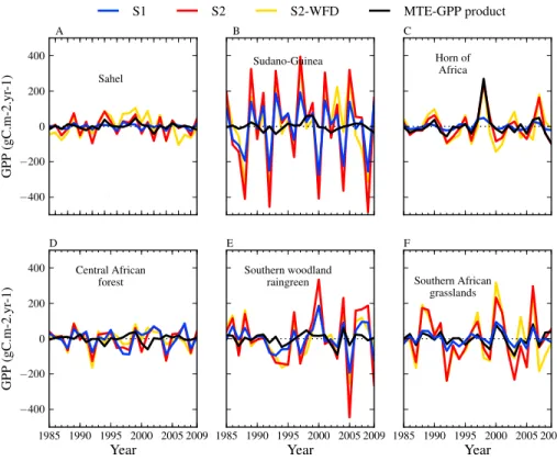
5.2.2. Gross Primary Productivity

On average, the IAV of GPP is comparable to the fAPAR IAV. The model-data agreement is higher over the Horn of Africa and the southern grasslands regions, as seen in Figure 3. Over these regions, ORCHIDEE has good GPP interannual correlations with the MTE-GPP product for both versions: r≈ 0.86 at 95% confidence interval in the Horn of Africa and the southern grasslands for the two-layer version (r≈ 0.77 at 95% confidence interval for the 11-layer version). The 11-layer version better captures the amplitude of IAV,

Table 5. Statistics of IAV for Latent Heat Flux (W m 2) Over the Six African Subregions; Same Presentation as in Table 3

Sahel Sudan-Guinea Horn of Africa

Central African Forest Southern Woodland Rain-Green Southern African Grasslands S1 x 26.4 71.7 24.1 100 59.3 25.4 σ 2.3 2.3 3.9 2.3 3.4 3.7 r 0.84 0.19 0.52 0.24 0.58 0.91 S2 x 28.7 69.8 28.2 74.8 56 28 σ 2.3 6.1 3 1 2.4 3.4 r 0.68 0.10 0.74 0.33 0.41 0.87 S2-FIXCO2 x 28.7 70.1 28.2 75.1 56.1 28 σ 2.3 6.2 3 1.1 2.4 3.4 r 0.68 0.11 0.74 0.33 0.41 0.87 S2-VARDEP x 26.2 64.7 27.6 74.1 53.6 27 σ 2 5.7 2.9 1.1 2.3 3.1 r 0.64 0.08 0.70 0.28 0.41 0.86 S2-WFD x 25.3 59.5 28.9 61 51.5 26.8 σ 2.1 4.7 4.1 2.5 2 3.1 r 0.59 0.07 0.41 0.51 0.19 0.8 MTE-LHF x 22.9 64 33.5 85.6 62 28 σ 1 1.15 2.9 0.5 1.1 2.2

Table 6. Statistics of IAV for Soil Moisture (%) Over the Six African Subregions; Same Presentation as in Table 3

Sahel Sudan-Guinea Horn of Africa

Central African Forest Southern Woodland Rain-Green Southern African Grasslands S1 x 0.10 0.15 0.13 0.22 0.14 0.11 σ 0.002 0.003 0.004 0.004 0.004 0.004 r 0.27 0.12 0.23 Missing 0.21 0.80 S2 x 0.49 0.5 0.49 0.84 0.58 0.49 σ 0.05 0.04 0.06 0.02 0.05 0.07 r 0.12 0.03 0.69 Missing 0.12 0.76 S2-FIXCO2 x 0.49 0.5 0.49 0.84 0.58 0.49 σ 0.05 0.04 0.06 0.02 0.05 0.07 r 0.12 0.04 0.64 Missing 0.12 0.76 S2-VARDEP x 0.38 0.42 0.43 0.7 0.44 0.30 σ 0.027 0.03 0.05 0.02 0.04 0.05 r 0.16 0.01 0.57 Missing 0.06 0.77 S2-WFD x 0.45 0.58 0.51 0.84 0.64 0.53 σ 0.08 0.04 0.06 0.02 0.04 0.07 r 0.26 0.09 0.59 Missing 0.12 0.77 SM-MW x 0.13 0.19 0.15 Missing 0.19 0.15 σ 0.01 0.01 0.01 Missing 0.02 0.01

Figure 2. Interannual time series of the detrended anomalies of the fraction of absorbed photosynthetically active radia-tion: comparison between the modeled fAPAR and the fAPAR3g GIMMS satellite product over the six African subregions.

Figure 3. Interannual time series of the detrended anomalies of the gross primary productivity: comparison between the modeled GPP (gC m 2yr 1) and the MTE-GPP data-driven model over the six African subregions.

Figure 4. Interannual time series of the detrended anomalies of the latent heatflux (W m 2): comparison between modeled ET and MTE-ET data-driven model over the six African subregions.

Figure 5. Interannual time series of the detrended anomalies per standard deviation unit (z-score): comparison between modeled surface soil moisture and SM-MW satellite product over the six African subregions.

particularly in the Sahel and the southern grasslands (SD≈ 0.8 and 0.95 times respectively of that MTE-GPP SD against 2.7 and 3.2 times respectively for the two-layer), but significantly underestimates the IAV over the Horn of Africa (SD≈ 0.3 times the one of MTE-GPP against SD ≈ 1.2 times for the two-layer) (Figures 3a, 3c, and 3f and Table 4). In central African forests (Figure 3d), the IAV of GPP is overestimated by all model versions (SD> 2.4 times of MTE-GPP SD). Like for the evaluation against fAPAR3g, the effect of meteorological forcing on IAV of GPP is significant (Figure 3), and the WFDEI forcing yields to a better agreement with MTE-GPP than the WFD forcing, in particular with smaller, more realistic anomalies during wet and dry years (especially in the Sahel, Horn of Africa, and the southern African grasslands).

5.2.3. Evapotranspiration

The modeled IAV of ET, shown in Figure 4, indicates the best performance of ORCHIDEE over the Sahel and the southern African grasslands, both for the 11- and two-layer versions (Figures 4a and 4f ). The modeled ET shows a too high IAV variability only in the Sudan-Guinea region, ET variability being comparable to MTE-ET IAV over the other African subregions. By contrast with GPP and fAPAR, the 11-layer version has greater interannual correlations with MTE-ET than in the two-layer version over the most part of Africa (see Table 5). As found for fAPAR and GPP, the ORCHIDEE 11-layer has less IAV of ET than the two-layer over all subregions and best matches the MTE-ET IAV. The comparison between IAV of GPP and ET (Figures 3 and 4) shows that the interannual SD of ET is better simulated by ORCHIDEE than the one of GPP, supporting either a more reliable reconstruction of ET than GPP by the MTE algorithm (section 3) or a better ability of ORCHIDEE to model ET than GPP, perhaps because the photosynthetic parameters of ORCHIDEE do not distinguish between different types of steppes, shrub lands, and savannahs. As for GPP, the WFDEI climate forcing provides better performance to reproduce the IAV of ET than the WFD forcing over all the regions, except for the central African forest region. The values of r range from 0.10 to 0.87 with the WFDEI climate forcing, compared to from 0.07 to 0.80 with WFD. However, the SD of the IAV of ET is slightly smaller with the WFD forcing especially over the Sudan-Guinea and the southern woodland rain-green regions.

5.2.4. Soil Moisture

The comparison of modeled soil moisture IAV with SM-MW is given in Figure 5. As pointed out for the evaluation of spatial gradients (section 5.1), the IAV of soil moisture in the two-layer version does not compare to SM-MW well, given that the model represents soil moisture over a much thicker than observed soil depth. The 11-layer soil model overcomes this shortcoming because it calculates the soil moisture profile in the soil. Soil moisture averaged in fourfirst layers representing the first centimeter of the soil is compared with SM-MW. In order to have the same range of IAV for the simulations and the SM-MW satellite data, we z-score transformed the (detrended) model output and the SM-MW observation. The detrended z-score (anomaly normalized by standard deviation) of soil moisture varies mainly between 2 and +3 for the ORCHIDEE simulations and the SM-MW data (Figure 5).

The results from the 11-layer version show that a multiple-layer soil hydrology allows to obtain more realistic soil moisture IAV, especially over semiarid and arid regions. Yet some anomalies are not captured by the model; the high positive SM-MW anomalies from 1988 to 1992 in the Sudan-Guinea region, and in 2002 over Sahel for instance. Like for otherfields, the southern African grasslands region has the best IAV correlation between ORCHIDEE results and SM-MW (r = 0.80 at 95% confidence interval with the 11-layer, and r = 0.76 at 95% confidence interval with the two-layer). Generally, the 11-layer version better matches the IAV of SM-MW, especially in the Sahel and the southern African grasslands (Figures 5a and 5f ), but the absolute SD (Table 6) remains between 65 and 70% lower than that of SM-MW. As for GPP and ET, the WFDEI meteorological forcing provides high IAV of soil moisture, and a better correlation with SM-MW observation, than the WFD forcing.

5.2.5. Summary of IAV

We found consistently that the ORCHIDEE 11-layer version improves the IAV of fAPAR, GPP (through the amplitude), ET, and soil moisture (through both correlation and amplitude) on arid and semiarid areas corresponding to savannahs and grasslands vegetation. The simulations are always more realistic over southern African grasslands, possibly because of a higher number of weather stations data that improves the quality of the meteorological forcing data for this region. The main result is that the SD of IAV is at least halved with the 11-layer version compared to the two-layer one and in better agreement with all the evaluation data products and over the most part of Africa. The only exception is for ET, where the 11-layer version has an IAV approximately close to the two-layer version. Note also that the quality of the climate forcing is important to

obtain more realistic modeled IAV results and that WFDEI gives systematically better performances than WFD. Variable orfixed soil depth in the two-layer version has no significant effect on the simulated variables (Tables 3 to 6). Finally, the effects of increasing CO2and land use change on the IAV of GPP, ET, and soil

moisture are negligible, although these drivers influence the trends of these three variables.

5.3. Contrast Between Wet and Dry Years

Rainfall is a key atmospheric driver of carbon and waterfluxes in Africa, and therefore, the ORCHIDEE model produces a contrasted response between wetter and drier periods in each region. In this section the performances of modeled soil moisture and GPP during highly wet (HW), wet (W), dry (D), and highly dry (HD) years, respectively, are examined. A highly wet year (respectively highly dry) is defined as a year for which yearly precipitation averaged (for considering climate forcing) over each grid cell is at least 10% higher (respectively lower) than the 10 year running mean in this grid cell. A wet year (respectively dry year) corresponds to when annual precipitation is between 0 and 10% above (respectively below) the 10 year running mean. Remark that with this definition, the selection of wet and dry years does differ between grid cells within a region.

5.3.1. GPP, fAPAR, and ET

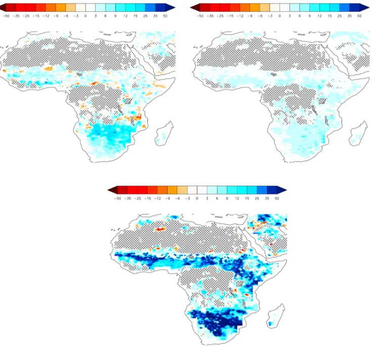
Here we focus on GPP only, as the maps of ET and fAPAR composite differences for HW, HD years allow to draw similar conclusions than for GPP and are not discussed further. Maps of the GPP composite difference between HW and HD years (absolute difference between the average of all HW years and the average of all HD years since 1979, hereafter calledΔGPP) is shown in Figure 6, for both versions of ORCHIDEE and for the MTE-GPP product. The MTE-GPP product shows high positiveΔGPP values over northern Sahel, the eastern Africa and the African southern grasslands. The simulated GPP shows a spatial pattern ofΔGPP similar to the MTE-GPP data product, except in some grid cells over the central African forest. However, the magnitude of the simulatedΔGPP is higher than the one from the data set. This larger modeled GPP contrast in response to rainfall compared to MTE-GPP is obtained regardless of the climate forcing (data not shown). The 11-layer version simulates a smaller ΔGPP than the two-layer version (especially in the southern grassland regions), but still larger than the MTE-derivedΔGPP (Figure 6). The geographic patterns of ΔGPP are less coherent when the contrast in “normal” W and D years is analyzed (Figure S2 in the supporting information) with different grid points taking either positive or negative values within the same subregion. ORCHIDEE reproduces this loss of spatial coherence in W and D maps, also found in MTE-GPP, regardless of the meteorological forcing or soil hydrology version used. This result is interesting because it suggests that extreme years offer more contrast, and thus a more coherent signal, to analyze the model responses to climate and evaluate them against observations.

5.3.2. Soil Moisture

Maps of the composite soil moisture difference between HW and HD years are given in Figure 7. As expected, SM-MW takes higher values during HW years over the whole continent, but there are some grid cells where ΔSM-MW remains negative even during HD years. The positive values of ΔSM-MW derived from satellite observation (Figure 7, top left) are the largest over the African southern grasslands region. The two-layer model version overestimatesΔSM-MW over the whole continent (Figure 7, bottom). Such a larger response than in the SM-MW observations can be explained by the integration of soil moisture over a 2 m soil depth. By contrast, the 11-layer version improves the situation greatly and results into a map ofΔSM rather similar to that obtained with SM-MW data over the most part of the continent, yet with too smallΔSM-MW values in southern Africa.

5.4. Interannual Sensitivities of Fluxes to Climate 5.4.1. Sensitivity to Rainfall

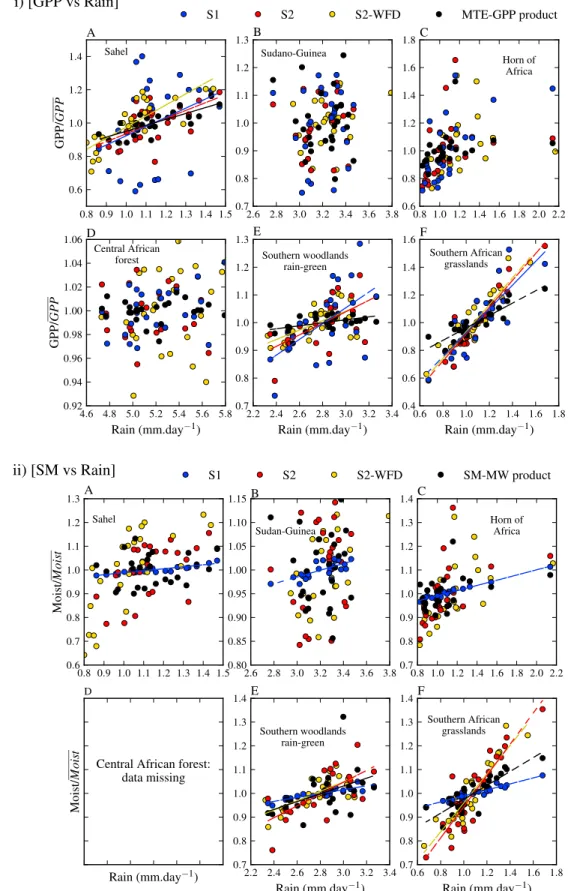
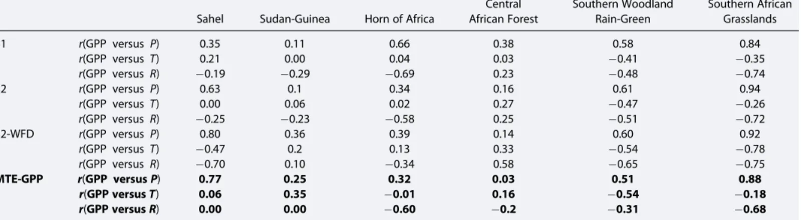
Figure 8 gives scatterplots of annual GPP versus rainfall IAV and of annual soil moisture versus rainfall. The southern African grasslands region has the strongest positive relationship between interannual GPP and rainfall IAV for both simulation and the MTE-GPP data-driven model (r> 0.80 at 95% confidence interval; see Table 7). The sensitivity of MTE-GPP to rainfall defined by the slope of a linear fit between GPP and rainfall is of 50 gC m 2per 100 mm of rainfall. In comparison, the sensitivity of ORCHIDEE GPP is too high over this region, suggesting that the model lacks negative feedbacks that stabilize the IAV of GPP (e.g., mechanisms of resistance of plants to drought related to an increased water use efficiency [Ponce-Campos et al., 2013] or shift in species composition during dry years allowing to sustain a higher GPP). The interannual sensitivity of GPP to rainfall in the 11-layer version is of 44 gC m 2per 100 mm and 175 gC m 2per 100 mm with the two-layer

version. The 11-layer version shows much better performance when evaluated for the sensitivity of GPP to rainfall. In other regions than southern African grasslands, the relationship between MTE-GPP and rainfall shows a larger scatter (in particular over Sudan-Guinea and central African forest regions; Figure 8i). Note that the relationship between GPP and rainfall in the Sahel region is higher for the MTE-GPP product (r = 0.77 at 95% confidence interval) than for ORCHIDEE GPP when using the WFDEI climate forcing (0.35 for the 11-layer version and 0.63 for the two-layer against 0.8 with the WFD climate forcing).

The relationship between soil moisture and rainfall (Figure 8ii) is strongest over southern African grasslands and southern woodland rain-green regions, for both modeled soil moisture and the SM-MW satellite product. The 11-layer version results show a strong and quasi-linear relationship between soil moisture and rainfall interannual anomalies over all African subregions (r> 0.80 at 95% confidence interval, except in the Sudan Guinea region; see Table 8), whereas the two-layer version exhibits more scatter (Figure 8ii). The correlation between the 11-layer soil moisture and rainfall is higher than 0.9 at 95% confidence interval over the

Figure 6.ΔGPP: High wet years minus high dry years. The difference is expressed in % of the sum of GPP of all high wet and high dry years since 1979. (top left) The MTE-GPP product, (top right) the result from S1 simulation (11-layer version), and (bottom) the result obtained with S2 simulation (two-layer version).

southern woodland rain-green and the southern African grasslands regions (against 0.68 and 0.9 at 90% confidence interval for the two-layer version, respectively). In comparison, the SM-MW satellite product has lower r values of≈ 0.47 in the southern woodland rain-green and 0.85 in the southern African grasslands. The stronger than observed relationship between modeled soil moisture and rainfall is possibly due to the fact thatfires are not properly represented in the both versions of ORCHIDEE tested in this study and that plant phenology is only triggered by soil moisture in the model, thus not capturing ecosystem recovery after burning. The interannual sensitivity of observed SM-MW to rainfall is of 3–4% per mm d 1of rain over these two southern regions, whereas the 11-layer simulation (the more realistic one) has a slope of about 1% per mm d 1. This is interesting to see that the modeled sensitivity of soil moisture to rainfall is dampened compared with the data product, whereas the GPP sensitivity was too high. It suggests altogether that the soil water stress of GPP (a simple linear function of moisture in the root zone with stress inception for root extractible water lower than 0.4; section 2) is too simply modeled in ORCHIDEE.

Figure 7.ΔSoil moisture: High wet years minus high dry years. The difference is expressed in % of the sum of soil moisture of all high wet and high dry years since 1979. (top left) The SM-MW satellite microwave product, (top right) the result from S1 simulation (11-layer version), and (bottom) the result obtained with S2 simulation (2-layer version).

Figure 8. (i) Relationship between GPP and rainfall (mm/d) over the six African subregions. (ii) Relationship between soil moisture and rainfall (mm/d) over the six African subregions.

5.4.2. Sensitivity to Near-Surface Air Temperature

The relationships between GPP, soil moisture, and air temperature show a large scatter over all subregions than with rainfall, and these relationships are systematically negative (Figure S4 in the supporting information), especially over the southern of Africa for the GPP. The correlations between modeled GPP and temperature are very weak over the continent (see Table 7), except in the southern woodland rain-green (r = 0.47 for the two-layer; r = 0.41 for the 11-layer version against r = 0.54 for MTE-GPP product). Note that the simulation using WFD climate forcing has high GPP correlation with temperature over the southern woodland rain-green (r = 0.78). Using a linearfit, we found, in the southern woodlands, a decrease of 265 gC m 2per °C for the two-layer, 110 gC m 2per °C for the 11-layer against 65 gC m 2per °C for the MTE-GPP product. The rp, partial correlation representing the correlation with temperature, controlling for rainfall colinearity, is

0.24 between the two-layer modeled GPP and temperature (rp= 0.17 for the 11-layer) compared to 0.38

for MTE-GPP product, suggesting a higher control of GPP by rainfall than by temperature. Analysis of multiple linear regressions representing the partial response of GPP as a function of rainfall, temperature, and radiation over the southern woodland rain-green region further shows that GPP increases with rainfall and slightly decreases with both temperature and radiation. According to multiple linear regression, the two-layer GPP increases by 65 gC m 2per 100 mm (33 gC m 2for the 11-layer against 15 gC m 2for MTE-GPP) and decreases rapidly with temperature and radiation respectively by 145 gC m 2per °C and 15 gC m 2per Wm 2respectively (50 and 5 gC m 2for the 11-layer against 44 and 1 gC m 2for MTE-GPP). Note that increasing atmospheric CO₂ tends to strengthen the relationship between GPP and rainfall over all the subregions and especially in the southern woodland rain-green. According to multiple linear regressions applied to the ORCHIDEE outputs, GPP increases by 65 gC m 2per 100 mm against 40 gC m 2per 100 mm in the simulation with constant CO2fixed at

its 1979 value. Increasing atmospheric CO₂also seems to limit the GPP decrease as a function of temperature

Table 7. Linear Correlation Between Year-to-Year GPP and the Main Climate Variables (P = Precipitation, T = Temperature at 2 m, and R = Solar Radiation) Over the Six African Subregions

Sahel Sudan-Guinea Horn of Africa

Central African Forest Southern Woodland Rain-Green Southern African Grasslands S1 r(GPP versus P) 0.35 0.11 0.66 0.38 0.58 0.84 r(GPP versus T) 0.21 0.00 0.04 0.03 0.41 0.35 r(GPP versus R) 0.19 0.29 0.69 0.23 0.48 0.74 S2 r(GPP versus P) 0.63 0.1 0.34 0.16 0.61 0.94 r(GPP versus T) 0.00 0.06 0.02 0.27 0.47 0.26 r(GPP versus R) 0.25 0.23 0.58 0.25 0.51 0.72 S2-WFD r(GPP versus P) 0.80 0.36 0.39 0.14 0.60 0.92 r(GPP versus T) 0.47 0.2 0.13 0.33 0.54 0.78 r(GPP versus R) 0.70 0.10 0.34 0.58 0.65 0.75 MTE-GPP r(GPP versus P) 0.77 0.25 0.32 0.03 0.51 0.88 r(GPP versus T) 0.06 0.35 0.01 0.16 0.54 0.18 r(GPP versus R) 0.00 0.00 0.60 0.2 0.31 0.68

Table 8. Same Statistics as in Table 7 for Soil Moisture

Sahel Sudan-Guinea Horn of Africa

Central African Forest Southern Woodland Rain-Green Southern African Grasslands S1 r(GPP versus P) 0.88 0.73 0.97 0.83 0.90 0.95 r(GPP versus T) 0.38 0.47 0.01 0.49 0.5 0.16 r(GPP versus R) 0.59 0.65 0.77 0.22 0.72 0.83 S2 r(GPP versus P) 0.54 0.28 0.53 0.68 0.68 0.90 r(GPP versus T) 0.25 0.07 0.16 0.33 0.51 0.17 r(GPP versus R) 0.13 0.31 0.73 0.08 0.57 0.6 S2-WFD r(GPP versus P) 0.73 0.47 0.56 0.64 0.70 0.91 r(GPP versus T) 0.48 0.26 0.03 0.06 0.65 0.77 r(GPP versus R) 0.65 0.42 0.54 0.23 0.62 0.74 SM-MW r(GPP versus P) 0.15 0.44 0.4 Missing 0.47 0.85 r(GPP versus T) 0.72 0.40 0.24 Missing 0.11 0.32 r(GPP versus R) 0.56 0.32 0.46 Missing 0.5 0.73

(the simulated GPP multilinear regression slope is of 145 gC m 2per °C in the two-layer, compared to 240 gC m 2per °C in thefixed CO₂simulation results). Using a spatially variable soil depth map for ORCHIDEE has a positive but very small effect on the relationship between rainfall and GPP, and a negative effect on the relationship between temperature and GPP (GPP has a temperature sensitivity of 120 gC m 2yr 1per °C with a variable soil depth, against 145 gC m 2yr 1per °C with a soil depth uniformlyfixed at 2 m). Like for GPP, the relationships between soil moisture and temperature or radiation drivers show a larger spread than that with rainfall. Yet SM-MW product better correlates with temperature anomalies over the Sahel (r = 0.72), whereas modeled soil moisture shows a weak correlation with temperature but in opposite sign between the two model versions (r = 0.25 for the two-layer and 0.38 for the 11-layer) over this region (see Table 8). Note that the simulated GPP and soil moisture using the WFD meteorological forcing have a stronger relationship with temperature over the southern woodland rain-green and the southern African grasslands (r≈ 0.65 and 0.77, respectively) than with the WFDEI forcing ( 0.57 and 0.6).

5.4.3. Sensitivity to Solar Radiation

The relationships between both GPP and soil moisture (Figure S3 in the supporting information) and solar radiation IAV are strong and negative over the Horn of Africa, the southern woodland rain-green, and southern African grassland regions but weak over all the other regions. The correlation between the two-layer GPP and solar radiation is 0.58, 0.51, and 0.72 in the Horn of Africa, the southern woodland rain-green, and the southern African grasslands, respectively, against 0.69, 0.48, and 0.74 for the 11-layer (see Table 7). However, the partial correlation between GPP and radiation (removing the effects of rainfall) is weak over the southern woodland rain-green and the southern African grassland regions (rp< 0.35 for all simulations) indicating a high

GPP dependence on rain, whereas GPP has less rainfall dependence in the Horn of Africa (r_p≈ 0.5). In comparison, the MTE-GPP product has smaller correlations of r = 0.6 (rp= 0.56) in the Horn of Africa, r = 0.31 (rp= 0.15)

in the southern woodland rain-green, and r = 0.7 (rp= 0.24) for the southern African grassland region. Over these

later regions, the two-layer version has a (negative) sensitivity to solar radiation of about 45 gC m 2per W m 2 compared to 13 gC m 2per W m 2for the 11-layer version, which is in better agreement with the sensitivity of MTE-GPP product to radiation, equal to 13 gC m 2per W m 2. Note that GPP variations associated with solar radiation changes are much lower than the one linked to rainfall and even to temperature. In the two-layer version, for instance, yearly GPP varies with radiation between 45 and 20 gC m 2per W m 2across subregions while it varies with temperature between 270 to 90 gC m 2per °C. Analysis of the response of soil moisture to solar radiation allowed us to draw similar conclusions than for GPP. Correlations between soil moisture and radiation are thus strong and negative over the Horn of Africa, the southern woodland rain-green and the southern African grasslands and weak over other regions (see Table 8).

6. Concluding Remarks

The African continent has an important role in the global carbon cycle yet not well quantified because of poor observation networks across the region. Ecological modeling combined with long-term remote sensing data can thusfill gaps in understanding how CO2and waterfluxes respond to climate and other drivers at various

temporal and spatial scales. This study highlights a large IAV of GPP, soil moisture, and ET over arid and semiarid ecosystems of Africa. We developed a method to evaluate the ORCHIDEE land surface model with two structurally different soil hydrology versions, which could be applied in the future to a larger ensemble of land surface models, e.g., the TRENDY [Sitch et al., 2013] or the Multi-scale Synthesis and Terrestrial Model Intercomparison Project (MsTMIP) [Huntzinger et al., 2013] model ensembles.

At the biome level, we found a greater sensitivity of grasslandfluxes to climate compared to closed forests. Clearly, the main drivers of GPP, ET, and soil moisture IAV are the precipitation and temperature variability. Because of the extent of grasslands and savannahs across Africa, this signature emerges at the continental scale. The ORCHIDEE simulations show a rather good agreement with satellite observations of regional IAV, especially for the 11-layer hydrology version, which is clearly superior to the two-layer bucket hydrology for soil moisture. This suggests that the two–bucket layer version buffers the effect of climate variability on ecosystems water budget, by maintaining either too large of a water reservoir for plants or by incorporating a too simple representation of rooting distributions and water access by plants. The fact that the 11-layer version of a rather generic land surface model gives good performance to reproduce the magnitude of the observed IAV of GPP and ET offers rather good prospects for using this category of models, with a specific

description of crop phenology, for hindcast testing and future forecast of plant productivity, and perhaps of crop yields over Africa. We also found that GPP and fAPAR were less sensitive to using the 11-layer version, which suggests that these quantities are controlled by additional processes than soil moisture, with possible lag effects and a strong influence of phenology.

For closed forests in central Africa, we found that the sensitivity of GPP to climate variability in the MTE-GPP data-driven product is smaller than in the ORCHIDEE simulations. This suggests either an underestimation of the IAV of GPP by the MTE algorithm, as previously noticed by Piao et al. [2013] with an ensemble of model results, or alternatively, that forests maintain a capacity to sustain carbon uptake during dry periods. Nevertheless, all the ORCHIDEE simulations appear to overestimate this capacity for fAPAR, while

underestimating (or having too high IAV) for ET, GPP, and soil moisture. Interestingly, ORCHIDEE soil moisture and GPP are too sensitive to rainfall in comparison to data products, indicating some error compensation mechanisms. We recommend developing model evaluation frameworks for the sensitivities offluxes to climate for future studies, such as attempted in section 5.4, because they bring more insights on model response. We also note that data-driven products used in this study are not direct observations and that the MTE interannual variance of GPP has been found in previous studies to be systematically smaller than the one from process-based land surface models [Anav et al., 2013; Piao et al., 2013]. One possible artifact of the MTE is that this algorithm is trained mainly on spatial gradients betweenflux towers and uses space for time to produce term series, with the overwhelming majority of sites located outside of Africa. In particular, MTE-GPP of savannahs has been found to be smaller than GPP deduced using Greenhouse Gases Observing SATellite (GOSAT)fluorescence data as a proxy [Frankenberg et al., 2011, 2012] or against Moderate Resolution Imaging Spectroradiometer GPP data sets [Zhao et al., 2005]. To further elucidate the causes for this discrepancy, more flux tower data are needed over arid and semiarid biomes, which cover approximately 45% of Africa. There are also other remote sensing based data sets for ET [Fisher et al., 2008; Jiménez et al., 2011; Mu et al., 2007; Vinukollu et al., 2011], though inherently direct satellite measurements limit the long temporal span we were interested in here. Choice of reference data sets for evaluating models can completely change evaluation results, so it is imperative that reference data sets contain spatiotemporally explicit and rigorously quantified uncertainties [Schwalm et al., 2013]. We also note that new proxy vegetation optical depth retrievals of the woody biomass fraction from microwave sensors [Andela et al., 2013], complementary to Advanced Very High Resolution Radiometer (AVHRR) NDVI and fAPAR products that are more related to the herbaceous fraction, are now available and should be used in future studies of the African CO₂and waterfluxes IAV.

References

Ackerley, D., B. B. Booth, S. H. Knight, E. J. Highwood, D. J. Frame, M. R. Allen, and D. P. Rowell (2011), Sensitivity of twentieth-century Sahel rainfall to sulfate aerosol and CO2 forcing, J. Clim., 24(19), 4999–5014.

Anav, A., P. Friedlingstein, M. Kidston, L. Bopp, P. Ciais, P. Cox, C. Jones, M. Jung, R. Myneni, and Z. Zhu (2013), Evaluating the land and ocean components of the global carbon cycle in the CMIP5 Earth system models, J. Clim., 26(18), 6801–6843.

Andela, N., Y. Liu, A. van Dijk, R. de Jeu, and T. McVicar (2013), Global changes in dryland vegetation dynamics (1988–2008) assessed by satellite remote sensing: Combining a new passive microwave vegetation density record with reflective greenness data, Biogeosci. Discuss., 10, 8749–8797.

Ball, J. T., I. E. Woodrow, and J. A. Berry (1987), A model predicting stomatal conductance and its contribution to the control of photosynthesis under different environmental conditions, in Progress in Photosynthesis Research, pp. 221–224, Springer, Netherlands.

Biasutti, M. (2013), Forced Sahel rainfall trends in the CMIP5 archive, J. Geophys. Res. Atmos., 118, 1613–1623, doi:10.1002/jgrd.50206. Biasutti, M., and A. Giannini (2006), Robust Sahel drying in response to late 20th century forcings, Geophys. Res. Lett., 33, L11706, doi:10.1029/

2006GL026067.

Botta, A., N. Viovy, P. Ciais, P. Friedlingstein, and P. Monfray (2000), A global prognostic scheme of leaf onset using satellite data, Global Change Biol., 6(7), 709–725.

Bruen, M. (1997), Sensitivity of hydrological processes at the land-atmosphere interface, in International Geosphere-Biosphere Program Symposium on Global Change and the Irish Environment, edited by J. Sweeney, Proc. Royal Irish Academy, Publ., Maynooth. Budyko, M. I. (1961), The heat balance of the Earth’s surface, Soviet Geogr., 2(4), 3–13.

Carsel, R. F., and R. S. Parrish (1988), Developing joint probability distributions of soil water retention characteristics, Water Resour. Res., 24(5), 755–769, doi:10.1029/WR024i005p00755.

Ciais, P., A. Bombelli, M. Williams, S. Piao, J. Chave, C. Ryan, M. Henry, P. Brender, and R. Valentini (2011), The carbon balance of Africa: Synthesis of recent research studies, Philos. Trans. R. Soc., A, 369(1943), 2038–2057.

Collatz, G. J., M. Ribas-Carbo, and J. Berry (1992), Coupled photosynthesis-stomatal conductance model for leaves of C4 plants, Funct. Plant Biol., 19(5), 519–538.

De Rosnay, P., and J. Polcher (1998), Modelling root water uptake in a complex land surface scheme coupled to a GCM, Hydrol. Earth Syst. Sci., 2, 239–255.

De Rosnay, P., M. Bruen, and J. Polcher (2000), Sensitivity of surfacefluxes to the number of layers in the soil model used in GCMs, Geophys. Res. Lett., 27(20), 3329–3332, doi:10.1029/2000GL011574.

Acknowledgments

This work is supported by the ClimAfrica project funded by the European Commission under the 7th Framework Program (FP7) (http://www.climafrica.net/ index_en.jsp). We are grateful to the GIMMS group for sharing the fAPAR3g data (we thank Zaichun Zhu and Ranga B. Myneni). Through Martin Jung, we are thankful to the Department of Biogeochemical Integration at the Max Planck Institute for Biogeochemistry for providing monthly gross primary pro-ductivity and evapotranspiration deduced from FLUXNET data from the La-Thuile-2007 synthesis effort (http://www.fluxdata.org).