HAL Id: halshs-01292901
https://halshs.archives-ouvertes.fr/halshs-01292901
Submitted on 17 Apr 2018HAL is a multi-disciplinary open access
archive for the deposit and dissemination of sci-entific research documents, whether they are pub-lished or not. The documents may come from teaching and research institutions in France or abroad, or from public or private research centers.
L’archive ouverte pluridisciplinaire HAL, est destinée au dépôt et à la diffusion de documents scientifiques de niveau recherche, publiés ou non, émanant des établissements d’enseignement et de recherche français ou étrangers, des laboratoires publics ou privés.
The diversity of socio-economic pathways and CO2
emissions scenarios: Insights from the investigation of a
scenarios database
Céline Guivarch, Julie Rozenberg, Vanessa Schweizer
To cite this version:
Céline Guivarch, Julie Rozenberg, Vanessa Schweizer. The diversity of socio-economic pathways and CO2 emissions scenarios: Insights from the investigation of a scenarios database. Environmental Modelling and Software, Elsevier, 2016, 80, pp.336-363. �10.1016/j.envsoft.2016.03.006�. �halshs-01292901�
The diversity of socio-economic pathways and CO2 emissions scenarios: insights from the investigation of a scenarios database
Céline Guivarcha,b, Julie Rozenbergb,c, Vanessa Schweizerd,e a Cired, Nogent-sur-Marne, France (guivarch@centre-cired.fr)
b Ecole des Ponts ParisTech, Champs-sur-Marne, France
c Climate Change Group Chief Economist Office, World Bank, Washington DC, USA. d National Center for Atmospheric Research (NCAR), Boulder, CO, USA e University of Waterloo, Department of Knowledge Integration, Waterloo, ON, Canada
Note: this text is a post –print of Guivarch, C., J. Rozenberg, and V. Schweizer. 2016. « The diversity of socio-economic pathways and CO2 emissions scenarios: Insights from the investigation of a scenarios database ». Environmental Modelling & Software Volume 80, Pages 336–353.
Abstract
The new scenario framework developed by the climate change research community rests on the fundamental logic that a diversity of socio-economic pathways can lead to the same radiative forcing, and therefore that a given level of radiative forcing can have very different socio-economic impacts. We propose a methodology that implements a “scenario discovery” cluster analysis and systematically identifies diverse groups of scenarios that share common outcomes among a database of socio-economic scenarios. We demonstrate the methodology with two examples using the Shared Socio-economic Pathways framework. We find that high emissions scenarios can be associated with either high or low per capita GDP growth, and that high productivity growth and catch-up are not necessarily associated with high per capita GDP and high emissions.
Keywords: scenario discovery, diversity, socioeconomic pathways, emissions scenarios, database.
Highlights
We adapt scenario discovery cluster analysis to explore socioeconomic scenario diversity.
A diversity of scenarios with high cumulative CO2 emissions is explored.
High emissions scenarios can be associated with either high or low per capita GDP growth.
Diverse scenarios can correspond to any of the Shared Socioeconomic Pathways domains.
Data availability
The database of scenarios outcome analyzed in this article, together with associated scenario drivers is available upon request.
1 Introduction
The scientific community has been developing a new generation of scenarios for climate change research and assessment (Moss et al. 2010) to replace the SRES scenarios (Nakicenovic et al., 2000) that have been widely used over the past decade.
One of the main innovations in this new generation of scenarios is relaxing the coupling between socioeconomic scenarios and emissions scenarios. Whereas previous generations of scenarios followed a sequential process starting from projecting different socioeconomic futures and then estimating the corresponding emissions, concentrations, radiative forcing and the ensuing climate change, the new generation initiated a parallel process (O’Neill and Schweizer, 2011; Ebi et al., 2014). This process starts with the selection of radiative forcing pathways (van Vuuren et al., 2011), from which investigations are proceeding in parallel: climate modellers simulate the climate change resulting from these radiative forcing pathways (Taylor et al., 2012) while scientists from the mitigation and adaptation communities develop socio-economic scenarios that could lead to these pathways.
The fundamental logic of this new architecture is the idea that each radiative forcing pathway is not associated with a unique socioeconomic scenario, and instead can result from different combinations of economic, technological, demographic, policy and institutional futures. This was a fundamentally important finding of the SRES scenarios, that alternative combinations of driving forces (e.g. population and economic growth) could lead to similar levels and structures of energy and land use. This new architecture has therefore the potential to overcome some of the main difficulty in scenario studies: “The more detail that one adds to the story line of a scenario, the more probable it will appear to most people, and the greater the difficulty they likely will have in imagining other, equally or more likely, ways in which the same outcome could be reached.” (Morgan and Keith, 2008). The new scenarios architecture offers the potential to help to identify a range of different technological, socioeconomic and policy futures that could lead to a particular concentration pathway. But exploring and managing the plethora of possible future trends in socio-economic development is also a great challenge for the developers of scenarios.
To address this challenge, it was decided to focus first on a small set of socio-economic pathways contrasted along two axes, the challenges for mitigation and the challenges for adaptation, in the Shared Socio-economic Pathways (SSP) framework (Nakicenovic et al., 2014; O’Neill et al., 2014). The Story and Simulation approach (Alcamo, 2008; O’Neill et al. 2015) was used to develop five storylines (O’Neill et al., 2015) and quantify five respective marker scenarios. To exploit the full potential of the new scenarios architecture, it was suggested to establish and utilize large databases of scenarios (Ebi et al., 2014) so as to allow scenario users to select a set of well-informed, self-consistent scenarios customized for their particular application. Indeed, the “Shared Socio-economic Pathways are canonical, but the canon is not exclusive”, as O’Neill et al. (2015) conclude, and for some uses of scenarios, it may be necessary to explore the diversity of socio-economic drivers that lead to specific outcomes.
Here we propose, with two example applications, a methodology that contributes to this longer-term research agenda by giving a quantified and systematic way to examine the diversity of socio-economic scenarios leading to similar outcomes. As noted by O’Neill et al. (2015), a novel feature of the SSP framework is that the relevant uncertainties of scenarios are associated primarily with alternative outcomes or results rather than the scenario drivers or inputs leading to outcomes. Nevertheless
alternative drivers should be considered in order to explore differences in outcomes. The methodology featured in this paper builds on Rozenberg et al. (2014), who constructed a large set of scenarios by varying scenario drivers systematically to explore the space of possible outcomes relevant to the SSP framework. This process generated hundreds of scenarios that comprise what we call a “scenarios database”. These scenarios were then classified into different scenario archetypes systematically rather than through developing only a few contrasting cases. Schweizer and O’Neill (2014) similarly assess a large number of scenarios by systematically varying the states of qualitative scenario elements. However only Rozenberg et al. (2014) apply this technique to the inputs of an integrated assessment model and run the model a large number of times to construct a database of integrated assessment outputs. Here, we investigate the scenario classifications further and select subsets of scenarios of interest, by their outcomes. To do this, we adapt a “scenario discovery” cluster analysis to uncover the diversity of driver combinations leading to the outcomes of interest.
The rest of this article is structured as follows. Section 2 presents the methods used. Section 3 describes two applications of this methodology. Because the development of the methodology was inspired by the SSP framework, the first application explores the diversity of scenarios classified as a particular type of SSP. The second application is not strictly linked to the SSP framework, as it explores more broadly the diversity of scenarios with high cumulative CO2 emissions. Section 4
discusses the results and methods and concludes.
2 Methods
The methodology proceeds in three steps. First we identify a priori the main driving forces (or main uncertainties) affecting the future outcomes of the system, such as population growth or fossil fuel reserves in the case of the human-climate system. Second we translate these driving forces into parameters for a model of the system studied, and we combine these parameters to build a large number of model runs. Note that the purpose of doing this is to systematically explore the implications of different combinations of drivers. Third we select a subset of scenario outcomes of interest, e.g. scenarios leading to high greenhouse gases (GHG) emissions. Because a diversity of drivers could have led to these outcomes, we iterate a “scenario discovery” cluster analysis to identify the diversity of combinations of drivers that lead to the selected subset of scenario outcomes. Section 2.1 describes the iteration of the scenario discovery cluster analysis. Section 2.2 presents the model we used and the driver or parameter sets that are systematically varied to build a database of scenarios.
2.1 Scenario discovery to uncover the diversity of scenarios
“Scenario discovery” cluster analysis provides a computer-assisted method of scenario development that applies statistical algorithms to databases of simulation model results to characterize the combinations of uncertain input parameter values (or “drivers”) most predictive of specified classes of results (Lempert et al. 2006). In other terms, the “scenario discovery” analysis is a systematic manner to find which combinations of the model input parameters lead to specific results of interest, i.e. cases where a given output variable is above or below a defined threshold or, more generally, cases where output variables are in specified areas of the results space. To describe the subset of scenarios of
interest, i.e. the cases where results are in specified areas of the results space, we define a binary indicator associated with scenarios. It takes the value 1 if scenarios belong to the subset of scenarios of interest and the value 0 otherwise.
We use the version of the PRIM (Patient Rule Induction Method) for the cluster analysis by Bryant and Lempert (2010). PRIM identifies several combinations of drivers, called “boxes”, and their coverage and density. Coverage is the fraction of scenarios consistent with the outcome indicators of interest, i.e. for which the indicator is equal to 1, that are also in the box (i.e. the combination of drivers) identified. Coverage corresponds to “recall” in the classification and information retrieval literatures. Density is the fraction of all scenarios in the box that are also in the subset of scenarios of interest. For example a density of 100% means that all scenarios in the box are in the subset of scenarios of interest; a density below 50% means that more than half of the scenarios in the box are, in fact, outside the subset of scenarios of interest. Density is analogous to “precision” or “positive predictive value” in the classification and information retrieval literatures. Since these two measures are generally in tension with one another, PRIM provides the user a set of options representing different trade-offs among density and coverage.
PRIM cluster analysis has been applied to a number of cases: pollution-control strategies (Lempert et al., 2006), long-term water planning (Groves and Lempert, 2007), the efficacy of a proposed renewable energy standard (Bryant and Lempert, 2010), low-carbon energy technologies (McJeon et al., 2011), near term policy choices for greenhouse gas transformation pathways (Isley et al., 2015), vulnerabilities of the port of Rotterdam (Halim et al., 2015), or the design of effective policies for stimulating bio-methane production in the Netherlands (Eker and van Daalen, 2015).
These
applications explicitly tie scenario discovery to policy design by identifying scenarios that
give rise to vulnerabilities for a proposed policy (i.e. that cause the policy to fail)
. In recent years, scenario discovery has been used independently from a specific policy design. For example, Gerst et al. (2013) use scenario discovery to “discover” plausible energy and economic futures, Kwakkel et al. (2013) to study the future of copper, and Rozenberg et al. (2014) to explore the space of challenges to mitigation and challenges to adaptation in the SSP framework. Other clustering methods also exist, in particular CART (Breiman et al., 1984), and have been applied to “discover” combinations of drivers leading to specific scenario outcomes (for example Gerst et al., 2013 use CART). For a comparison between PRIM and CART cluster analysis, one may refer to Lempert et al. (2008), Hadka et al. (2015) and Kwakkel and Jaxa-Rozen (forthcoming). However, all of those applications of cluster analysis were focusing on identifying the main combination of drivers predictive of a specific scenario outcome, and did not specifically focus on the possible diversity of combinations of drivers.H
ere we propose a particular implementation of the “scenario discovery” cluster analysis to uncoverthe diversity of uncertain driver combinations (boxes), within a subset of scenarios of interest by outcome. This implementation consists of an iteration of the scenario discovery cluster analysis with the PRIM algorithm (Figure 1). At each step of the iteration, the box with the maximum density is retained. We call this box a scenario “family”. For the following step, the box is kept in the database of scenarios, but switched from the subset of scenarios of interest to the subset of scenarios not of interest. The scenario discovery cluster analysis is then applied again to the remaining members of the subset of scenarios of interest by outcome. The iteration stops when the scenario discovery analysis does not find any new box with a density higher than 50%, i.e when the scenarios in the box are more outside the subset of scenarios of interest than inside. This implementation is different from the usual
implementation of PRIM iterations, in which the box is removed from the database at each step of the iteration. Keeping the scenarios in the database, but removing them from the subset of scenarios of interest, forces the algorithm to find diverse boxes, because at each step the condition “not being in the previously identified boxes” is added. This modified implementation, when more than one iteration is made, allows uncovering several combinations of drivers that lead to the specific outcomes of interest, or several scenario “families” that achieve similar outcomes. The analysis and comparison of the different families of drivers inform the diversity of scenarios characterized by a specific type of outcome.
Define subset of scenarios of
interest as the scenarios that lead
to outcome of interest
Run scenario
discovery cluster
analysis (PRIM) for
the scenarios with
binary indicator at
value 1
Select the box with
the highest density
Is density
>50% ?
No
Stop
Set the binary indicator at
value 0 for the scenarios in
the box
Define outcome of interest
Keep selected box to define
the scenario family
identified for this iteration
Yes
Define a binary indicator
associated with scenarios, taking
the value 1 if scenarios belong to
the subset of scenarios of interest
Figure 1: Iteration of scenario discovery cluster analysis to uncover the diversity of combinations of scenario drivers leading to scenario outcomes of interest.
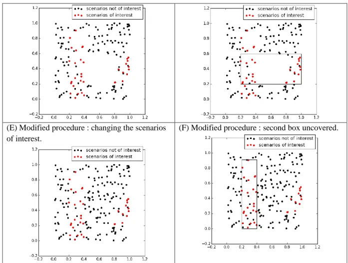
Figure 2 gives a visual explanation of the modification procedure we suggest in the scenario discovery iteration, and illustrates why it may improve the diversity of boxes uncovered by the PRIM algorithm. The illustration uses a simple dataset with two uncertain variables, x and y, represented in panel A of the Figure (x along the X-axis and y along the Y-axis), where the red dots are the scenarios of interest. At the first step of the scenario discovery, as shown in Panel B, the PRIM algorithm would find a box where x is between 0.4 and 0.8 and y between 0.2 and 0.6, because there is a high density of scenarios of interest in this area.
In the original procedure of PRIM, the box uncovered would be removed from the dataset, as shown in Panel C, and the PRIM algorithm would be run on the remaining data. In that case, the second box uncovered would plausibly be the box drawn in Panel D. This second box contains the empty space left by removing the previous box, because the hill climbing optimization algorithm in PRIM is not considering the impact of the previously removed data points.
In the modified procedure we propose, instead of removing the box previously uncovered from the dataset, they are kept but changed from the subset of scenarios of interest to the subset of scenarios not of interest, as show in Panel E. Because the previous box is not removed, but simply no longer of interest, the hill climbing optimization algorithm used by PRIM accounts for these data points and the optimization procedure is penalized if it included data points that are in the first box. As a result, the algorithm will search for a second box that minimizes overlap with the first box. A possible box that PRIM would then find is shown in Panel F. As can be seen, this new box does not overlap anymore with the first box. Therefore this modified procedure improves the diversity of boxes uncovered, compared to the original procedure.
(A) Example dataset. (B) First box uncovered by PRIM algorithm.
(C) Original procedure : removing the box from the dataset.
(E) Modified procedure : changing the scenarios of interest.
(F) Modified procedure : second box uncovered.
Figure 2 : Visual illustration of the modification to the scenario discovery procedure proposed.
2.2 Building a database of scenarios
The database of scenarios was built with the Imaclim-R model (Waisman et al., 2012). It is a multi-region and multi-sector model of the world economy that represents the intertwined evolution of technical systems, energy demand behavior and economic growth. It combines a Computable General Equilibrium (CGE) framework with bottom-up sectoral modules in a hybrid and recursive dynamic architecture. Furthermore, it describes growth patterns in second-best worlds with market imperfections, partial uses of production factors and imperfect expectations. The model represents endogenous Gross Domestic Product (GDP) and structural change, energy markets and induced technical change. The scope of GHG gases represented is restricted to CO2 emissions from fossil fuel
combustion. The main exogenous assumptions are demography and labour productivity growth, the maximum potentials of technologies (renewable, nuclear, carbon capture and storage, electric vehicles…), the learning rates decreasing the cost of technologies, fossil fuel reserves, the parameters of the functions representing energy-efficiency in end-uses, the parameters of the functions representing energy-demand behaviors and life-styles (motorization rate, residential space, evolutions in consumption preferences…). An extended description of the model is available at http://www.imaclim.centre-cired.fr/IMG/pdf/imaclim_v1.0.pdf. Details about the model structure and results with respect to various aspects (energy technologies, energy efficiency, fossil fuels, macroeconomy) can be found in the publications listed in the Appendix. In the landscape of Integrated Assessment Models (IAMs), Imaclim-R can be labeled as a recursive dynamic General Equilibrium Model with a medium variety of low-carbon technologies. Diagnostics of its response to carbon
pricing places it as a “low response” model, which means that a given carbon price leads to a relatively low abatement and high cost per abatement compared to other IAMs (Kriegler et al., 2015).
In the Imaclim-R model, GDP is endogenous, but it is driven by exogenous demographic trends (total population growth and active population growth) and exogenous trends of labor productivity (see Appendix). Structural change and technical change are also endogenous and induced by relative price movements. The latter can be influenced exogenously by the potentials for new technologies (e.g. maximum market share, learning rates) and the potentials for energy efficiency (e.g. the reaction of energy input consumption to energy prices).
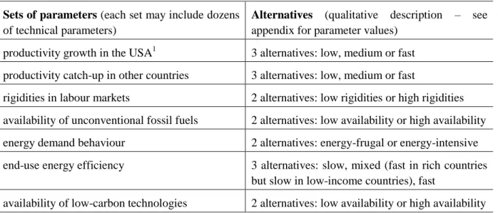
To explore the multi-dimensional space spanned by uncertain model input, we followed a method previously developed in (Rozenberg et al. 2014). We first identified the model parameters that can have an impact a priori on scenario outcomes in terms of emissions and GDP in particular. The model parameters are then grouped into seven parameter sets presented in Table 1. For each parameter set, two or three alternatives were built with contrasting parameter values (Table 1).
Table 1: Description of the uncertain alternatives Sets of parameters (each set may include dozens
of technical parameters)
Alternatives (qualitative description – see
appendix for parameter values) productivity growth in the USA1 3 alternatives: low, medium or fast productivity catch-up in other countries 3 alternatives: low, medium or fast
rigidities in labour markets 2 alternatives: low rigidities or high rigidities availability of unconventional fossil fuels 2 alternatives: low availability or high availability energy demand behaviour 2 alternatives: energy-frugal or energy-intensive end-use energy efficiency 3 alternatives: slow, mixed (fast in rich countries
but slow in low-income countries), fast
availability of low-carbon technologies 2 alternatives: low availability or high availability
The description of the parameters in each set and their respective values are given in the Appendix.
The combinations of these alternative assumptions generated 432 scenarios. All are baseline scenarios, i.e. no climate policy is implemented. This choice is consistent with the SSP framework, which separates socio-economic pathways and climate policy assumptions, the latter being represented by “shared climate policy assumptions” (Kriegler et al., 2014).
The 432 scenarios results range from about 1600 GtCO2 to about 2800 GtCO2 in terms of cumulative
CO2 emissions in 2100 since the pre-industrial period. This range is just slightly smaller than the range
1 Historically the USA has been the leading country for productivity growth (it is the country with the highest
productivity levels). It is retained as the leader for the representation chosen of productivity growth with a leader and catch-up to the leader by other regions.
covered by the baseline scenarios in the IPCC AR5 database, which contains baseline scenarios ranging from about 1400 GtCO2 to about 3000 GtCO2. Global per capita GDP in 2100 ranges from
twice to eleven times its value in 2014. This range of results is also comparable to the range covered by baseline scenarios in the IPCC AR5 database, in which global per capita GDP in 2100 ranges from approximately 2.5 to 9.5 its value today.
Even though a large ensemble of scenarios is created through this approach, it should be acknowledged that only a portion of the full uncertainty space is investigated, and that results are conditional to the choices of sets of parameters to vary and of the alternative values tested. Other sets of parameters or other alternative values might be relevant to investigate. Obviously, the impact of an uncertain driver on the results depends on the numerical assumptions behind each state of the driver. This limitation is inherent to our methodology, but cannot be avoided when accounting for uncertainty in a large number of model input parameters.
The grouping of parameters into seven parameter sets excludes the exploration of some “unusual” combinations of factors, i.e. within a given parameter set, parameters values are assumed to co-vary and other combinations of parameters values are currently not explored. This choice of grouping parameters results from two main reasons: (i) the interpretability of results that requires a limited number of “meaningful” drivers, and (ii) the model runtime2
that limits the number of runs possible. Further study could disaggregate some of the parameter sets, if results indicate that specific parameter sets are important for the output of interest.
Moreover, the sets of parameters are varied independently from each other, which neglects the possible cross-correlation of some of the sets of parameters, e.g. the cross correlation of productivity drivers with technology availability or energy-efficiency drivers. Neglecting such cross-correlations tends to produce a range of results that is too broad, because some scenarios in the set may not be internally consistent. At the same time, insisting on consistency in scenarios may reduce the ability to identify plausible surprising futures.
Furthermore, no objective probabilities can be assigned to scenarios because we are in a case of uncertainty, and not in a case of risks where objective probabilities of parameters are known (Grubler and Nakicenovic, 2001; Cooke, 2015). The likelihood of any particular scenario would have to be interpreted as subjective, in the Bayesian sense, and conditional to the model structure used and the alternative values tested. Therefore, the distribution of results cannot be interpreted as an objective distribution of probabilities of outcomes (or probabilities in the frequentist sense). For this reason, we will not study the distribution of results itself or present mean or median values, but instead consider the ranges of results and the position of scenario outcomes relative to some thresholds of interest.
3 Applications
We demonstrate this methodology with two example applications. Both utilise the same database of scenarios described in the previous section. For both applications, we used the PRIM implementation for R (Bryant, 2015), with its default parameterization3.
2 The Imaclim-R model typically runs in 1 hour on a Core i7 3.1GHz processor. 3
Note that a different implementation or parameterization may lead to slightly different results. In particular, Kwakkel and Jaxa-Rozen (forthcoming) has shown that implementing a more lenient objective function, and a
3.1 Diversity of scenarios where “challenges to adaptation” or “challenges to mitigation” dominates
Our first application is closely linked to the Shared Socioeconomic Pathways (SSP) framework. The SSPs are defined by their relative socioeconomic challenges to mitigation or challenges to adaptation (Figure 3, left panel). Mitigation and adaptation challenges may co-vary (i.e. low, medium, or high challenges, which are SSPs 1-3), or they may not (i.e. high adaptation challenges coupled with low mitigation challenges (SSP4), or high mitigation challenges coupled with low adaptation challenges (SSP5)).
In this analysis of scenarios with the SSP framework, we measured mitigation challenges by global CO2 emissions at the end of the century and adaptation challenges by the GDP per capita of
low-income countries4 at the end of the century to map our 432 baseline scenarios into the SSP space (Figure 3, right panel). High global emissions contribute to the challenge for mitigation because that would mean more emissions to eliminate to reach a given temperature or concentration level. Low per capita GDP in low-income countries contributes to the challenge for adaptation because that would mean less financial capacities for adaptation. However, we acknowledge that the measures chosen are only a simplification and that challenges to mitigation or adaptation are rich concepts that include a wide range of socio-economic factors (O’Neill et al., 2014; Rothman et al., 2014). Alternative measures to map scenario outcomes into the challenges space could be tested. For example, in Rozenberg et al. (2014), two other indicators are tested:
the GDP losses from a mitigation policy
reducing emissions to stabilize radiative forcing at a given level (a target at 3.7 Wm
−2) for
challenges to mitigation, and the share of jobs in agriculture in developing countries for
adaptation challenges.
We then normalized results for these quantitative indicators to arrive at indicators for the SSP scenario space with domain and range [0,1]. Since our scenarios were derived from one model, we interpreted domain boundaries relative to the distribution of the 432 scenarios.
W
e chose to make SSP domains the same size with a diamond-shaped domain in the center corresponding to SSP2.modified objective for handling multinomial classified data (which is the case of our data), in the PRIM
algorithm leads to slightly different results, with better coverage scores in the example studied by the author.
4
We define low-income countries as the three countries/regions with the lowest per-capita GDP in 2014. They correspond to the regions « India », « Africa » and « Rest of Asia » in our modelling framework.
Figure 2 :Left panel: The SSP scenario space and five scenario narratives titles (reproduced from O’Neill et al. 2015). Right panel: Mapping of 432 IMACLIM-R scenarios into the SSP scenario space.
We focused on the off-diagonal (SSP4 and SSP5) domains and applied the methodology to uncover the diversity of combinations of drivers of scenarios in that domain of relatively low global emissions and relatively low GDP per capita in low-income countries in the long term. These “off-diagonal” domains of the challenge space in the SSP framework, i.e. a domain where challenges to mitigation and to adaptation are not correlated but one challenge dominates, are of special interest because “off – diagonal” scenarios may appear less intuitive, as discussed by O’Neill et al. (2015):
Previous narratives used in climate change scenarios conveyed the general nature of future development through key characteristics such as economic growth, regional integration, societal sustainability and environmental sustainability. These characteristics were used to define sets of representative futures that cover a desired space of uncertainty for use in scenario analysis. Interestingly, the types of narratives (and their combinations into sets) employed in past scenarios exhibited similarities and recurrent themes (…). This fact may point to the relevance of these themes to climate change analysis, but may also reflect a certain lock-in to
a particular way of framing environmental scenario analysis (emphasis added; p. 3 of 12).
The authors also say at the start of their results section, “Somewhat more discussion is provided for those SSPs, notably SSP4, which are less well represented in previous scenario exercises” (p. 4 of 12). Because of the underrepresentation of scenarios like SSP4 and SSP5, when we constructed our database of scenarios, we intentionally chose parameters sets and alternative values such that some combinations could a priori lead to scenario outcomes in the off-diagonal domains. Given the alternatives of parameter sets chosen, and the indicators chosen to measure the challenges to mitigation and the challenges to adaptation, the SSP4 domain results in being the most populated domain in our database (37% of scenarios are in SSP4 domain). This might indicate that there are several different combinations of drivers that lead to outcomes in the SSP4 domain, which justifies the interest to apply a systematic method to uncover this potential diversity. However, this relative “frequency” of scenario outcomes in the SSP4 domain should not be interpreted in terms of likelihood of SSP4 because, as discussed at the end of section 2.1, no objective probability can be attached to individual scenarios and therefore scenarios results cannot be analysed in a frequentist framework. Scenarios in the SSP5 domain are less numerous: they represent only 5% of all scenarios.
We first focused on the SSP4 domain. The iteration of the scenario discovery cluster analysis on the subset of scenarios of interest, defined as the scenarios in the SSP4 domain, identified 7 families of scenarios, which can be further combined into 4 groups according to their leader productivity growth driver value and their location in the SSP4 domain (Table 2 and Figure 4). All families are characterized by low fossil fuel availability, but differ with respect to the other drivers.
The first family has low or medium leader productivity growth, energy-intensive demand behaviours and low or mixed energy efficiency. The scenarios from this family are located in the bottom-right corner of the domain (red crosses in Figure 4), i.e. they are characterized by the lowest emissions and lowest GDP per capita in low-income countries relative to the other scenarios in the database. Indeed, energy-intensive demand behaviours and low or mixed energy efficiency, combined with low availability of fossil fuels, lead to high energy prices, which hinder growth.
The second group of scenario families (families n°2, 5 and 6) also have relatively low emissions, but slightly higher GDP per capita in low-income countries (they are more to the left of the domain: light blue, blue and black stars in Figure 4). Here, either energy-frugal demand behaviours or high energy efficiency allow growth to be faster while keeping emissions low (relative to the other scenarios in the database).
The third group of scenarios families (families n°3 and 7) share similar drivers: low productivity catch-up and low labour market rigidities. The corresponding scenarios are scattered in the SSP4 domain (light green and dark green circles in Figure 4), because various combinations of leader productivity growth and energy-demand behaviours lead to various locations in terms of GDP per capita and emissions.
The last family of scenarios (n°4) has medium or fast leader productivity growth, high labour-market rigidities, energy-intensive behaviours and low or mixed energy efficiency. The scenarios in this family are located in the top-right corner of the domain (orange triangles in Figure 4), i.e. with relatively high emissions and low GDP per capita in low-income countries compared to other scenarios in the domain. The medium or fast labour productivity growth in the leading country, combined with energy-intensive behaviours, leads to relatively high growth in developed countries and relatively high emissions, but high labour-market rigidities and low energy efficiency in developing countries slow growth in those countries.
Table 1: Families of scenarios uncovered by PRIM analysis for the SSP4 domain. The families are numbered in the order of PRIM discovery, but organized in the table according to their similarities in terms of state of the leader growth driver (dark and light grey shading are used to differentiate the groups with similar leader growth
driver). Density and coverage results are reported to the remaining scenarios with binary indicator at value 1 at each time step, the values corresponding to the initial subset of scenarios of interest are given in parenthesis when different. The density and coverage scores are also given for the four clusters taken together, with respect
to the initial subset of scenarios of interest. Note that the coverage of the four clusters taken together is slightly less than the sum of coverage values for each cluster, because some scenarios are in several clusters.
Figure 3 : Positions of the scenarios families in the SSP4 quadrant.
PRIM clusters 1 2 5 6 3 7 4 Seven clusters
together 100% 100% 73% 100% 65% 67% 100% (93%) (88%) (100%) 31% 14% 16% 20% 12% 17% 15% (9.6%) (9.0%) (7.7%) (9.6%) (7.7%) (7.7%) low medium fast low medium fast low high energy-frugal energy-intensive low mixed high low high low high
rigidities in labor markets Scenarios in SSP4 domain
leader productivity growth
productivity catch-up coal and unconventional
fossil fuels availability energy demand behaviors
energy efficiency availability of low-carbon
technologies
density 98%
The results show that several different combinations of drivers can lead to similar outputs in emissions and per capita GDP growth in low-income countries. In particular, combinations of drivers with either high productivity catch-up and/or high leader productivity growth exist in the SSP4 domain. Furthermore, outcomes in terms of inter-regional inequalities vary within and between scenarios families uncovered. For illustration, the per capita GDP of low-income countries at the end of the century for the scenarios in the SSP4 domain varies between 44% and 82% of the global per capita GDP at the end of the century (compared to 20% today). In all scenarios, inter-regional inequalities are reduced, due to catch-up assumptions, but at various speeds. The inter-regional inequality outcome is not an outcome that is a differentiating characteristic between scenario families uncovered, except for family 5, which is characterized by low inter-regional inequalities (the per capita GDP of low-income countries at the end of the century is above 65% of the global per capita GDP), driven by relatively low productivity growth in high-income countries and relatively fast productivity catch-up by other countries). However, interpreting our results in terms of inequalities, and the comparison with the SSP4 narrative entitled “Inequality – A road divided” from O’Neill et al. (2015) is difficult because there is no intra-regional inequality explicitly represented in our modelling framework, whereas the SSP4 narrative emphasizes inequalities both between and within countries.
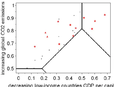
Applied to the SSP5 domain, the scenario discovery iteration finds only one family of scenarios with a density higher than 50% (Table 3 and Figure 5). This family is defined by the combination of high leader productivity growth, medium or high productivity catch-up, low rigidities in labour markets, high availability of fossil fuels and energy-intensive demand behaviours. The first three drivers explain the high GDP growth; the last two explain that it is energy- and carbon-intensive growth. The density of this family of scenarios is relatively low (67%), and a number of scenarios characterized by this combination of drivers are located in the SSP3 domain (Figure 5).
The fact that only one family of scenarios is uncovered is linked to the low number of scenarios in the SSP5 domain. This difficulty in finding scenarios corresponding to SSP5 was already discussed in Rozenberg et al. (2014). It is linked to the structure of the Imaclim-R model, where GDP growth is affected by energy consumption and efficiency. If energy demand is too high—and energy efficiency too low—energy prices are so high that GDP growth is significantly reduced, especially in developing countries. This explains why there are few scenarios with high economic growth in low-income countries and high baseline emissions. This result however depends on the indicator considered, and taking a different indicator for challenges to mitigation could help for finding SSP5 scenarios (see Rozenberg et al., 2014, for an example with an alternative indicator for challenges to mitigation).
Table 3: Family of scenarios uncovered by PRIM analysis for the SSP5 domain.
Figure 5 : Position of the scenarios family in the SSP5 quadrant.
The finding that high emissions scenarios are not necessarily associated with high GDP per capita growth motivates our second application, which is not directly linked to the SSP framework but studies more broadly high cumulative CO2 emissions scenarios.
3.2 Diversity of scenarios with high cumulative CO2 emissions
Our second example focuses on scenarios with high cumulative CO2 emissions. While a 2°C target is
an approved objective in international negotiations on climate change, the continued rise of greenhouse gases emissions makes it a more and more difficult target to achieve (Guivarch and Hallegatte, 2013) and, if continued further, increase the risk to reach 3°C, 4°C or more by the end of
PRIM clusters 1 density 67% coverage 36% low medium fast low medium fast low high energy-frugal energy-intensive low mixed high low high low high energy efficiency availability of low-carbon technologies rigidities in labor markets Scenarios in SSP5 domain
leader productivity growth
productivity catch-up coal and unconventional
fossil fuels availability energy demand behaviors
the century. Acknowledging this risk, some studies have focused on the evaluation of impacts and adaptation challenges for high temperature increase (e.g. New et al., 2011; and IPCC, 2014a for a review). But damages for climate change impacts and capacities to adapt will also depend on future socio-economic worlds. It is therefore important to explore what a high emissions/high temperature change world would look like in socio-economic terms. There are a few archetypes of such high emissions worlds in the literature, e.g. the RCP 8.5 scenario (Riahi et al., 2011) and SRES A2 and A1F (Nakicenovic et al., 2000), but there remains a relatively small number of such high emissions scenarios (IPCC, 2014b, chapter 6) and the diversity of socio-economic conditions that could lead to high emissions has not been studied systematically. The following example is thus the first study of this type.
We selected the scenarios that lead to cumulative CO2 emissions since the pre-industrial period above 2400 GtC. This threshold corresponds to the cumulative CO2 emissions in the RCP8.5 scenario (IPCC, 2013), for which global surface temperature change by the end of the 21st century, relative to the average from year 1850 to 1900, is projected to be likely to exceed 4°C by the end of this century. This subset of scenarios represents 15% of the scenarios in our scenarios ensemble (Figure 6).
The iteration of the scenario discovery algorithm, as described above, uncovers 4 families of scenarios, or combinations of uncertain drivers (Table 4). Details of PRIM results at each step of the iteration are given in Appendix 1. All families of scenarios uncovered share two common drivers: high availability of coal and unconventional fossil fuels and energy-intensive demand behaviours. However they differ on the other drivers, in particular the leader productivity growth and productivity catch-up. This result is consistent with elements in the recent literature, in particular two findings. First, it is consistent with Schweizer and Kriegler (2012), who found that a coal-powered growth storyline was both very self-consistent and under-represented in the SRES scenarios. It is also in line with Mouratiadou et al. (2015) who found, with a sensitivity analysis of the REMIND model results, that assumptions on fossil fuel availability have a strong impact on baseline emissions, via an effect on carbon intensity mainly.
One family (n°3) is characterized by fast leader productivity growth and fast productivity catch-up by other countries, combined with high availability of fossil fuels and energy-intensive demand behaviours. It resembles the SSP5 narrative from O’Neill et al. (2015) entitled “fossil-fuel development – taking the highway”, which emphasizes that “the push for economic and social development is coupled with the exploitation of abundant fossil fuel resources and the adoption of resource and energy intensive lifestyles around the world. All these factors lead to rapid growth of the global economy”.
Another family (n°1) shares the same combination of drivers except for productivity catch-up, which is low or medium. In this family, GDP per capita growth is fast in high-income countries, but slower in other countries. Emissions are still high globally, in part due to high emissions from high-income countries, but also because the slower catch-up from other countries is associated (by assumption) with higher population in those countries. This results in slower energy intensity improvement in lower income countries, the combination of which also results in high emissions in those countries.
The two other families (n°2 and 4) have medium labour productivity growth. Emissions are nevertheless in the high range because the availability of low carbon technologies is low (family n°2) or because energy efficiency is low (family n°4). These families could be interpreted as closer to the SSP3 narrative from O’Neill et al. (2015) that describes a world in which “economic development is
slow, consumption is material-intensive … [there is] growing resource intensity and fossil fuel dependency … and slow technological change”, or close to the socio-economic pathways underlying RCP 8.5, which combines assumptions about high population and relatively slow income growth with modest rates of technological change and energy intensity improvements.
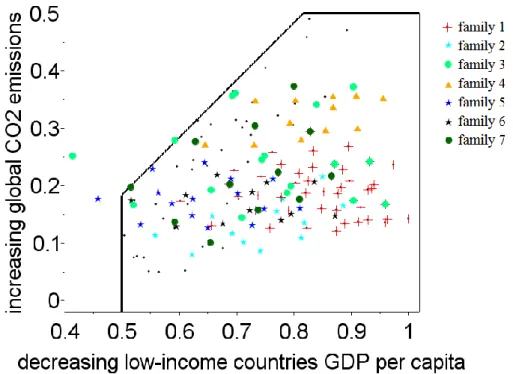
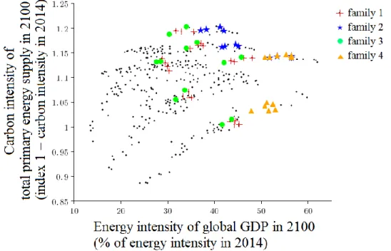
The four families also vary in some outputs, notably in the per capita GDP growth (Figure 6, X-axis), but also the energy intensity of GDP and the carbon intensity of energy (Figure 7). Family 3 is characterized with high per capita growth, family 1 with relatively high per capita growth and families 2 and 4 with relatively low growth at the global scale (Figure 6). The fact that similar outcomes in terms of cumulative emissions can be associated with different outcomes in terms of per capita GDP, can be explained by two elements: (i) the role of population as a scaling factor, and (ii) the role of feedbacks between growth and energy intensity and/or carbon intensity. On the first element, in particular, scenarios in family 3 have higher per capita GDP growth than scenarios in family 1, but also lower population (see Appendix 1); with both factors compensating each other such that emissions are similar. Families 1 and 3 have a similar distribution of energy intensity and carbon intensity (Figure 7), which range from moderate to high for both; but scenarios characterized with high energy intensity have moderate carbon intensity, and scenarios with high carbon intensity have moderate energy intensity. On the second element, the feedbacks between growth and energy intensity tend to associate higher growth with faster energy intensity improvement, due to faster capital turn-over and faster technical change. In particular, scenarios in families 2 and 4 are characterized by lower per capita growth than scenarios in families 1 and 3, but also slower improvement in energy intensity, especially family 4 in which the driver “energy efficiency” is low (see Appendix 1). The combination of both opposite effects leads to similar emissions. Scenarios in family 2 have high carbon intensity – because of the low availability of low-carbon technologies – and relatively high energy intensity (Figure 7); whereas scenarios in family 4 have very high energy intensity – because of low energy efficiency – that is not compensated by lower carbon intensity.
These results highlight that high emissions scenarios are not necessarily associated with high per capita GDP growth, but can be associated with relatively low per capita GDP growth, if counterbalanced by high population growth and/or slow energy intensity improvement.
Table 4 : Families of scenarios uncovered by PRIM analysis. The grey boxes represent the combinations of
parameters values corresponding to each family of scenarios identified. Density and coverage results are reported to the remaining scenarios with binary indicator at value 1 at each time step; the values corresponding to the initial subset of scenarios of interest are given in parenthesis when different. The density and coverage scores are
also given for the four clusters taken together, with respect to the initial subset of scenarios of interest. Note that the coverage of the four cluster taken together is slightly less than the sum of coverage values for each cluster,
because a few (4) scenarios are in both cluster 2 and cluster 4 (which can be seen on Figure 6 as well).
PRIM clusters 1 2 3 4 Four clusters together 100% 67% 92% 58% (92%) 42% 24% 44% 50% (14%) (19%) (19%) low medium fast low medium fast low high energy-frugal energy-intensive low mixed high low high low high rigidities in labor markets
High cumulative emissions scenarios
leader productivity growth
productivity catch-up coal and unconventional
fossil fuels availability energy demand behaviors
energy efficiency availability of low-carbon
technologies
density 89%
Figure 6 : The 432 scenarios plotted according to the global per capita GDP in 2100 (X-axis) and the global
cumulated CO2 emissions since the pre-industrial period (Y-axis). Families of scenarios uncovered by PRIM analysis are materialized with red crosses (family 1), blue stars (family 2), green circles (family 3) and orange
triangles (family 4).
Figure 7 : The 432 scenarios plotted according to the energy intensity global GDP in 2100 (X-axis) and the
carbon intensity of total primary energy supply in 2100 (Y-axis). Families of scenarios uncovered by PRIM analysis are materialized with red crosses (family 1), blue stars (family 2), green circles (family 3) and orange
triangles (family 4).
4 Discussion and conclusion
In light of the two applications, the methodology we propose to systematically iterate a scenario discovery cluster analysis can be instrumental in providing insights on the diversity of drivers in socio-economic scenarios leading to specific outcomes. We discovered four combinations of drivers leading to high cumulative emissions scenarios, and seven combinations of drivers leading to scenarios with high global emissions and low per capita GDP in low-income countries at the end of the century. However, we were unable to find more than one combination of drivers leading to scenarios with high global emissions and high per capita GDP in low-income countries. This result is due to the structural characteristics of the model used to build the database.
When multiple combinations of drivers are uncovered, some are quite similar and share several of the same drivers, in particular in the application on the SSP4 domain. For the ease of interpretation, the analyst may need to group the combinations uncovered according to their similarities, or the methodology may be further adapted to automatically propose grouping of the combinations uncovered according to the drivers they share.
Moreover, the order in which families of scenarios are uncovered matters in the methodology, because at each step of the iteration, the scenario discovery algorithm is applied to a subset of scenarios
defined as the original subset of scenarios of interest and the negation of the previously identified families of scenarios. For some applications, this might hold implications for the interpretation of uncovered families of scenarios, and it might be necessary to adapt the methodology so that the order in which families of scenarios are uncovered would not matter.
Notwithstanding these limitations, the results highlight that high emissions scenarios are not necessarily associated with high per capita GDP growth, and that high leader productivity growth and high productivity catch-up are not necessarily associated with high per capita GDP growth and high emissions. These results have implications for financing capacities for mitigation actions, and for vulnerability, impacts and adaptation. In particular, a high emissions world with low or medium per capita GDP may pose larger challenges for financing capacities than a high emissions world associated with high per capita GDP.
Further development of the methodology would include further explorations of the differences between the families of scenarios identified, in particular the exploration of their respective dynamic behaviour.
This methodology may be useful when scenario diversity is a question worth exploring. Therefore it may be relevant for future developments within the SSP framework, or in other scenario studies where there is a plethora of uncertain drivers of future developments. In particular, it represents a possibility to blend the narrative and quantitative scenario approaches by using quantitative data and analysis to inform the process of selecting a few scenarios and suggesting which storylines are most policy relevant to develop. It could be used to develop alternative narratives and quantified scenarios that are hard to imagine. In this paper, we found alternative versions of scenarios with high emissions and “off diagonal” challenges that differ from those already featured in the scholarly literature.
Acknowledgements
The authors wish to thank Jan Kwakkel for very detailed and relevant comments on previous versions of this article, and for his suggestion of a visual illustration that we followed to elaborate figure 2. The authors also thank three anonymous reviewers for their comments, which helped improve this text. The National Center for Atmospheric Research is funded by the National Science Foundation and managed by the University Corporation for Atmospheric Research.
References
Alcamo, Joseph. 2008. « The SAS approach: combining qualitative and quantitative knowledge in environmental scenarios ». Environmental futures: The practice of environmental scenario analysis 2: 123-50.
Breiman, L., Friedman, J.H., Olshen, R.A., Stone, C.J., 1984. Classification and Regression
Trees. Chapman & Hall, Washington, D.C.
Bryant BP, Lempert RJ (2010) Thinking inside the box: a participatory, computer-assisted approach to scenario discovery. Technol Forecast Soc Chang 77:34–49.
Bryant B.P. (2015).
Scenario Discovery Tools to Support Robust Decision Making,
documentation of the ‘sdtoolkit’ package for R. available at
https://cran.r-project.org/web/packages/sdtoolkit/sdtoolkit.pdf
Cooke, Roger M. 2015. « Messaging Climate Change Uncertainty ». Nature Climate Change
5 (1): 8-10.
Ebi, Kristie L., Stephane Hallegatte, Tom Kram, Nigel W. Arnell, Timothy R. Carter, Jae Edmonds, Elmar Kriegler, et al. 2014. « A New Scenario Framework for Climate Change Research: Background, Process, and Future Directions ». Climatic Change 122 (3): 363-72.
Eker, S., van Daalen, C., 2015. A model-based analysis of biomehtane production in the Netherlands and the effectivenss of the subsidization policy uncer uncertainty. Energy Policy 82: 178-196.
Friedman JH, Fisher NI (1999) Bump hunting in high-dimensional data. Stat Comput 9:123–143
Gerst, M. D., P. Wang, et M. E. Borsuk. 2013. « Discovering plausible energy and economic
futures under global change using multidimensional scenario discovery ». Environmental
Modelling & Software, Thematic Issue on Innovative Approaches to Global Change
Modelling, 44 (juin): 76-86. doi:10.1016/j.envsoft.2012.09.001.
Guivarch, C. and Hallegatte, S. 2013. ’2°C or not 2°C ?’ Global Environmental Change, Vol
23, Issue 1, p 179-192.
Groves, D. G., et R. J. Lempert. 2007. « A new analytic method for finding policy-relevant
scenarios ». Global Environmental Change 17 (1): 73-85.
Grübler, Arnulf, et Nebojša Nakicenovic. 2001. « Identifying dangers in an uncertain
climate ». Nature 412 (6842): 15.
Hadka, D., Herman, J.D., Reed, P.M., Keller, K., 2015. OpenMORDM: An open source
framework for many objective robust decision making. Environmental Modelling & Software
74: 114-129.
Halim, R.A., Kwakkel, J.H., Tavasszy, L.A., 2015. A scenario discovery study of the impact
of uncertainties in the global container transport system on European ports. Futures (in press).
IPCC, 2013: Summary for Policymakers. In: Climate Change 2013: The Physical Science
Basis. Contribution of Working Group I to the Fifth Assessment Report of the
Intergovernmental Panel on Climate Change [Stocker, T.F., D. Qin, G.-K. Plattner, M.
Tignor, S.K. Allen, J. Boschung, A. Nauels, Y. Xia, V. Bex and P.M. Midgley (eds.)].
Cambridge University Press, Cambridge, United Kingdom and New York, NY, US
IPCC, 2014a: Climate Change 2014: Impacts, Adaptation, and Vulnerability. Part A: Global
and Sectoral Aspects. Contribution of Working Group II to the Fifth Assessment Report of the
Intergovernmental Panel on Climate Change [Field, C.B., V.R. Barros, D.J. Dokken, K.J.
Mach, M.D. Mastrandrea, T.E. Bilir, M. Chatterjee, K.L. Ebi, Y.O. Estrada, R.C. Genova, B.
Girma, E.S. Kissel, A.N. Levy, S. MacCracken, P.R. Mastrandrea, and L.L. White (eds.)].
Cambridge University Press, Cambridge, United Kingdom and New York, NY, USA, 1132
pp.
IPCC, 2014b: Climate Change 2014: Mitigation of Climate Change. Contribution of Working
Group III to the Fifth Assessment Report of the Intergovernmental Panel on Climate
Change [Edenhofer, O., R. Pichs-Madruga, Y. Sokona, E. Farahani, S. Kadner, K. Seyboth,
A. Adler, I. Baum, S. Brunner, P. Eickemeier, B. Kriemann, J. Savolainen, S. Schlömer, C.
von Stechow, T. Zwickel and J.C. Minx (eds.)]. Cambridge University Press, Cambridge,
United Kingdom and New York, NY, USA.
Isley, S.C., Lempert, R.J., Popper, S.W., Vardavas, R., 2015. The effect of near-term policy choices on long-term greenhouse gas transformation pathways. Global Environmental Change 34: 147-158.
Kriegler, E., Edmonds, J., Hallegatte, S., Ebi, K., Kram, T., Riahi, K., Winkler, H., Van Vuuren, D.P., 2014. A new scenario framework for climate change research: The concept of Shared Climate Policy Assumptions. Climatic Change 122(3), 401-414.
Kriegler, Elmar, Nils Petermann, Volker Krey, Valeria Jana Schwanitz, Gunnar Luderer,
Shuichi Ashina, Valentina Bosetti, et al. 2015. « Diagnostic indicators for integrated
assessment models of climate policy ». Technological Forecasting and Social Change 90,
Part A : 45-61.
Kwakkel, Jan H., Willem L. Auping, et Erik Pruyt. 2013. « Dynamic scenario discovery under
deep uncertainty: The future of copper ». Technological Forecasting and Social Change 80
(4): 789-800.
Kwakkkel, J.H., Jaxa-Rozen, M., (forthcoming). Improving scenario discovery for handling
heterogeneous uncertainties and multinomial classified outcomes. Environmental Modelling
& Software.
Lempert, R. J., D. G. Groves, S. W. Popper, et S. C. Bankes. 2006. « A general, analytic
method for generating robust strategies and narrative scenarios ». Management Science,
514-28.
Lempert, Robert J., Benjamin P. Bryant, et Steven C. Bankes. 2008. « Comparing algorithms
for scenario discovery ». RAND, Santa Monica, CA.
McJeon, H. C., L. Clarke, P. Kyle, M. Wise, A. Hackbarth, B. P. Bryant, et R. J. Lempert.
2011. « Technology interactions among low-carbon energy technologies: What can we learn
from a large number of scenarios? ». Energy Economics 33 (4): 619-31.
Morgan, M. G., and D. W. Keith. 2008. « Improving the way we think about projecting future energy use and emissions of carbon dioxide ». Climatic Change 90 (3): 189-215.
Moss, Richard H., Jae A. Edmonds, Kathy A. Hibbard, Martin R. Manning, Steven K. Rose, Detlef P. van Vuuren, Timothy R. Carter, et al. 2010. « The next generation of scenarios for climate change research and assessment ». Nature 463 (7282): 747-56.
Mouratiadou, Ioanna, Gunnar Luderer, Nico Bauer, et Elmar Kriegler. 2015. « Emissions and
Their Drivers: Sensitivity to Economic Growth and Fossil Fuel Availability across World
Regions ». Climatic Change, mars, 1-15. doi:10.1007/s10584-015-1368-4.
Nakicenovic, Nebojsa, Joseph Alcamo, Gerald Davis, Bert de Vries, Joergen Fenhann, Stuart Gaffin, Kenneth Gregory, et al. 2000. Special Report on Emissions Scenarios : a special report of Working Group III of the Intergovernmental Panel on Climate Change.
Nakicenovic, Nebojsa, Robert J. Lempert, and Anthony C. Janetos. 2014. « A Framework for the Development of New Socio-Economic Scenarios for Climate Change Research: Introductory Essay ». Climatic Change 122 (3): 351-61.
New, M., Liverman, D., Schroder, H., Anderson, K. 2011. Four degrees and beyond: the potential for a global temperature increase of four degrees and its implications. Phil. Trans. R. Soc. A 369, 6-19.
O’Neill, B. C., and V. Schweizer. 2011. « Projection and prediction: Mapping the road ahead ». Nature Climate Change 1 (7): 352-53.
O’Neill, Brian C., Elmar Kriegler, Keywan Riahi, Kristie L. Ebi, Stephane Hallegatte, Timothy R. Carter, Ritu Mathur, and Detlef P. van Vuuren. 2014. « A new scenario framework for climate change research: The concept of shared socioeconomic pathways ». Climatic Change 122 (3): 387-400.
O’Neill, Brian C., Elmar Kriegler, Kristie L. Ebi, Eric Kemp-Benedict, Keywan Riahi, Dale
S. Rothman, Bas J. van Ruijven, et al. 2015. « The roads ahead: Narratives for shared
socioeconomic pathways describing world futures in the 21st century ». Global
Environmental Change. (in press)
Riahi, Keywan, Shilpa Rao, Volker Krey, Cheolhung Cho, Vadim Chirkov, Guenther Fischer,
Georg Kindermann, Nebojsa Nakicenovic, et Peter Rafaj. 2011. « RCP 8.5—A scenario of
comparatively high greenhouse gas emissions ». Climatic Change 109 (1-2): 33-57.
Rothman, D.S., Romero-Lankaro, P., Schweizer, V.J., Bee, B.A. 2014. Challenges to
adaptation: a fundamental concept for the shared socio-economic pathways and beyond.
Climatic Change 122 (3), 495-507.
Rozenberg, Julie, Céline Guivarch, Robert Lempert, and Stéphane Hallegatte. 2014. « Building SSPs for Climate Policy Analysis: A Scenario Elicitation Methodology to Map the Space of Possible Future Challenges to Mitigation and Adaptation ». Climatic Change 122 (3): 509-22.
Sassi, O., R. Crassous, J. C. Hourcade, V. Gitz, H. Waisman, et C. Guivarch. 2010.
« Imaclim-R: a modelling framework to simulate sustainable development pathways ».
International Journal of Global Environmental Issues 10 (1): 5-24.
Schweizer, Vanessa Jine, et Elmar Kriegler. 2012. « Improving environmental change
research with systematic techniques for qualitative scenarios ». Environmental Research
Letters 7 (4): 044011.
Schweizer, Vanessa J. and Brian C. O’Neill. 2014. “Systematic construction of global
socioeconomic pathways using internally consistent element combinations”. Climatic Change
122 (3): 431-445.
Taylor, K.E., Stouffer, R.J., Meehl, G.A., 2012. A summary of the CMIP5 experiment design. Bull. Am. Meteorol. Soc. 93, 485-498.
Waisman, Henri, Céline Guivarch, Fabio Grazi, and Jean Charles Hourcade. 2012. « The Imaclim-R Model: Infrastructures, Technical Inertia and the Costs of Low Carbon Futures under Imperfect Foresight ». Climatic Change 114 (1): 101-20.
Appendix 1 – Details of PRIM iterations results
Application on the diversity of scenarios where “challenges to adaptation” or “challenges to mitigation” dominates
Table A1 shows the boxes given by PRIM algorithm at each step in the iteration for SSP4 domain, with their respective density and coverage results (only boxes with density above 50% are shown, because with a density below means that scenarios characterized by the combination of drivers identified are more outside than inside the subset of scenarios of interest). Table A2 gives the resampling test results at each step of the iteration for SSP4 domain.
The quasi-p-value test and the resampling test are diagnostic tools to evaluate the statistical significance of the constraints on inputs (or drivers) proposed by the scenario discovery algorithm. The quasi-p-value estimates the likelihood that PRIM constrains some input purely by chance: low quasi-p-values (e.g. below 0.05) give strong evidence that the constraint on the given input is statistically significant. The resampling test evaluates a scenario definition by assessing how frequently the same definition arises from different samples of the same database. Two resampling tests are in fact given – one in which the algorithm generates a scenario matching as closely as possible the coverage of the original box, and one in which it matches the density. These two tests often but not always generate identical results. Resampling tests values closer to 1 indicate a constraint on the corresponding input has high statistical significance, while values closer to 0 indicate low statistical significance. More details on both tests are given in Bryant and Lempert (2010).
Steps in the iteration
boxes 1 2 3 4 1 2 3 4 5 density 100% 98% 88% 72% 100% 96% 85% 65% 57% coverage 31% 46% 61% 96% 14% 20% 26% 30% 55% low medium fast low medium fast
low 2.5E-04 4.1E-20 9.3E-21 4.1E-25 2.9E-04 1.1E-05 3.7E-06 9.5E-06 1.6E-08
high
energy-frugal 1.9E-05 7.1E-07 9.4E-04 1.6E-01
energy-intensive 4.4E-02 2.1E-04 5.2E-05
low mixed high low high low
high 6.1E-01 1.8E-01 7.6E-02 9.3E-02 5.8E-02
availability of low-carbon technologies rigidities in labor markets Scenarios in SSP4 domain
energy efficiency 6.4E-02 1.1E-03 1.1E-01 1.7E-02 1.1E-02 productivity catch-up 5.1E-01
coal and unconventional fossil fuels availability energy demand behaviors
leader productivity growth
5.1E-01 4.8E-01 1.1E-01
Table A1: Boxes uncoverd by PRIM algorithm at each time step in the iteration of the scenario
discovery for SSP4 domain. Quasi-p-values for individual drivers are given in the shaded cells.
Steps in the iteration
boxes 1 2 1 2 3 4
density 65% 55% 100% 83% 58% 50% coverage 12% 19% 15% 18% 26% 33%
low medium
fast 1.9E-06 3.8E-03
low 1.1E-01 2.3E-01
medium fast
low 4.8E-03 3.4E-03 2.4E-04 3.7E-04 2.5E-04 2.4E-04
high energy-frugal
energy-intensive 9.0E-02 6.2E-02 9.9E-02 1.7E-01
low mixed
high
low 5.5E-01 6.0E-01
high
low 2.8E-01
high 2.0E-01 1.0E-01 6.6E-02 6.4E-02
availability of low-carbon technologies rigidities in labor markets
productivity catch-up coal and unconventional
fossil fuels availability energy demand behaviors
energy efficiency 1.1E-01 Scenarios in SSP4 domain
leader productivity
growth 2.0E-01
3 4
Steps in the iteration
boxes 1 2 3 1 2 3 1 2 density 73% 61% 53% 100% 83% 58% 67% 61% coverage 16% 20% 26% 20% 25% 36% 17% 23% low medium fast
low 1.9E-02 5.5E-03
medium fast
low 3.2E-03 2.4E-03 1.5E-03 2.4E-04 3.7E-04 2.5E-04 1.9E-02 7.0E-03
high
energy-frugal 3.2E-03 2.4E-02 1.2E-02
energy-intensive 1.3E-02 1.4E-02 9.5E-03
low 1.0E-02 4.6E-03 2.0E-02
mixed
high 1.8E-06 1.5E-06 1.2E-04
low
high 1.9E-02 8.9E-03
low 5.0E-02 1.1E-01
high 3.2E-02 2.4E-02
4.7E-01
availability of low-carbon technologies rigidities in labor markets
energy efficiency productivity catch-up
1.5E-01 2.9E-01
coal and unconventional fossil fuels availability energy demand behaviors
5 6 7 leader productivity growth 2.4E-01 1.1E-01 Scenarios in SSP4 domain for equivalent coverage for equivalent density for equivalent coverage for equivalent density for equivalent coverage for equivalent density for equivalent coverage for equivalent density
leader productivity growth 0.4 0.4 0.1 0.1 0.1 0.1 0.1 0.1
productivity catch-up 0 0 0.4 0.4 0.7 0.7 0.1 0.1
coal and unconventional fossil fuels availability 1 1 1 1 1 1 1 1
energy demand behaviors 0.9 0.9 0.8 0.8 0.2 0.2 0.5 0.5
energy efficiency 1 1 0.3 0.3 0.1 0.1 0.1 0.1
availability of low-carbon technologies 0 0 0 0 0.3 0.3 0.2 0.2
rigidities in labor markets 0 0 0.5 0.5 0.2 0.2 0.9 0.9