Applications performance on reconfigurable computers

Applications Performance on Reconfigurable

Computers

by

Jang Don Kim

Submitted to the Department of Electrical Engineering

and Computer Science in Partial Fulfillment of the

Requirements for the Degree of

Master of Engineering in Electrical Engineering and

Computer Science

at the

MASSACHUSETTS INSTITUTE OF TECHNOLOGY

May 23, 1997

Copyright 1997 Jang Don Kim. All Rights Reserved.

The author hereby grants to M.I.T. permission to

reproduce distribute publicly paper and electronic copies

of this thesis and grant others the right to do so.

A uthor

...

....

.

... t

...

...

epaement of Electrical Engineering and Computer Science

May 23, 1997

Certified by

... ,...

..

...

...

/

Pro

ant

Agarwal

Thesis Supervisor

A ccepted by

... ...

...-

.. . -

., ·..

, ...

Arthur C. Smith

Chairman, Department Committee on Graduate Theses

Applications Performance on Reconfigurable Computers

by

Jang Don Kim

Submitted to the

Department of Electrical Engineering and Computer Science May 23, 1997

In Partial Fulfillment of the Requirements for the Degree of Master of Engineering in Electrical Engineering and Computer Science

Abstract

Field-programmable gate arrays have made reconfigurable computing a possibility. By placing more responsibility on the compiler, custom hardware constructs can be created to expedite the execution of an application and exploit parallelism in computation. Many reconfigurable computers have been built to show the feasibility of such machines, but applications, and thus compilers required to map those applications to the hardware, have been lacking. RAWCS (Reconfigurable Architecture Workstation Computation

Structures) is a methodology for implementing applications on a generic reconfigurable platform.[3] Using RAWCS, two applications, sorting and the travelling salesperson problem, are studied in detail. The hardware constructs and techniques required to map these applications to a reconfigurable computer are presented. These techniques involve the numerical approximation of complex mathematical operations in the simulated annealing solution to the travelling salesperson problem in order to make it possible to map those operations to a reconfigurable platform. It is shown that these integer

approximations have no adverse effects on the solution quality or computation time over their floating point counterparts.

Thesis Supervisor: Anant Agarwal

Acknowledgements

The entire RAW Group contributed significantly to this project. Thanks go to Jonathan Babb for coming up with, creating the framework for, and pushing everyone to work on the RAW benchmark suite. Thanks also go to Matthew Frank and Anant Agarwal for their support, advice, and intoxicating enthusiasm.

I would also like to give thanks to Maya Gokhle who introduced me to the field of reconfigurable computing and helped me to take my first steps.

Table of Contents

1 Introduction ... 13

1.1 Field-Programmable Gate Arrays ... ... 13

1.2 Reconfigurable Computers ... 15

1.3 Overview of This Thesis ... 18

2 R A W C S ... ... 2 1 2.1 Introduction ... 2 1 2.2 Compilation Methodology ... ... 21 2.3 Target Hardware ... ... 23 3 S ortin g ... ... 2 5 3.1 Problem Description ... 25

3.2 Algorithms to Find a Solution ... 25

3.3 RAWCS Implementation ... ... 26

4 Travelling Salesperson Problem ... 31

4.1 Problem Description ... 31

4.2 Algorithms for Finding a Solution ... 31

4.3 RAWCS Implementation ... ... 33

5 Numerical Approximations for Simulated Annealing ... .. 39

5.1 Numerical Approximations... ... 39

5.2 D ata Sets ... . ...40

5.3 B ase C ase ... ... ... 40

5.4 Linear Temperature Schedule ... ... 41

5.5 Probability Approximation ... 47

5.6 Finding the Best Numerical Approximation... ... 49

6 Conclusions ... 55

6.1 M erge Sort ... ... 55

6 .2 T S P ... _{... 56}

Appendix A Merge Sort Source ... ... ... 59

A .1 driver.c ... . . ... 59 A .2 library.v ... ... 63 A .3 generate.c ... ... 66 Appendix B TSP Source ... 71 B .1 driver.c ... ... 7 1 B.2 library.v...82 B.3 generate.c ... 94

Appendix C Data Sets ... 99

C. 1 80 City TSP... 99

A ppendix D ... . . ... 99

C .2 640 C ity T SP ... 100

Appendix E Results of Base Case... 101

D. 1 80 City TSP Solution ... 101

D.2 640 City TSP Solution ... 102

List of Figures

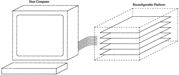
Figure 1.1 Typical Setup of a Reconfigurable Computer ... 15

Figure 3.1 Merge Sort Hardware Construct...28

Figure 3.2 Merge Sort Performance Results... ... 29

Figure 4.1 Parallelizing Energy Change Calculation... ... 37

Figure 5.1 Temperature Cooling Schedule for Base Case...41

Figure 5.2 Performance of Base Case on Two Problems ... 42

Figure 5.3 Linear Cooling Schedules... 43

Figure 5.4 Performance of Linear Cooling Schedules... ... 44

Figure 5.5 Performance of Best Linear Schedule ... 46

Figure 5.6 Performance of Exponential Approximation... ... 48

Figure 5.7 Performance of Best Approximation... ... 50

Figure 5.8 Performance of Best Numerical Approximation ... 51

Figure 5.9 Improved Computation Time ... 53

Figure 6.1 Parallel Implementation of Exponential Approximation ... 57

Figure C .1: 80 C ity TSP ... ... 99

Figure C .2: 640 C ity TSP ... ... 100

Figure D. 1: Solution for 80 City TSP ... 101

List of Tables

Chapter 1

Introduction

1.1 Field-Programmable Gate Arrays

Field-Programmable Gate Arrays (FPGAs) were introduced by Xilinx Corp. in 1986. FPGAs are a class of integrated circuits that is capable of emulating any digital circuit within physical limitations. A digital circuit is specified in software and is then translated into a bitstream in a process known as synthesis. This bitstream is then downloaded into the FPGA which gives the chip the necessary information to configure itself to emulate the original digital circuit.

Hardware

The FPGA is usually composed of three kinds of building blocks: configurable logic blocks (CLBs), input/output blocks (IOBs), and interconnection networks.[20] A CLB can be configured to perform any Boolean function of a given number of inputs. IOBs are arrayed along the edge of the chip and are used to communicate from the interior of the chip to the pins on the outside of the chip. The interconnection networks serve two main functions within the FPGA: to connect the I/O blocks to the CLBS and to connect the CLBs to each other.

Synthesis

There are two levels at which a circuit can be described for synthesis. At the highest level, a behavioral description in a behavioral Hardware Description Language (HDL) specifies the behavior of a circuit with no implementation details. The logic components and interconnect required to realize the behavior of the circuit are determined by the synthesis tools in a process called behavioral synthesis. The output of behavioral synthesis

is a structural description of the circuit generally called a netlist. Behavioral synthesis is a very complex problem and is not yet well understood. A circuit designer can circumvent the behavioral synthesis stage by describing the target circuit in structural form. This reduces synthesis time and avoids the behavioral synthesis tool which is prone to producing the incorrect structural description. Many HDLs today, such as Verilog and VHDL, offer tools that can translate circuit descriptions that utilize both structural and behavioral constructs giving the designer more flexibility.[24][25]

Logic synthesis is a series of steps that translates the structural netlist to the target

bitstream. In the first step, the translator converts the structural netlist to a format understood by the mapping software. The technology mapper then replaces the components in the translated netlist with FPGA-specific primitives and macros. It analyzes timing behavior using the FPGA-specific components to ensure the mapping does not violate the timing constraints of the original design. The partitioner then divides up the mapped netlist among the FPGA chips available on the target system while maximizing gate utilization and minimizing inter-chip communication. The global placer maps each partition into individual FPGAs while minimizing system communication. The global router determines inter-chip routing, and the FPGA APR (automated place-and-route) converts the individual FPGA netlists to configuration bitstreams which are then downloaded into the FPGA.[6]

Applications

FPGAs are used in two broad classes of applications: logic emulation[10] and reconfigurable computing. In logic emulation, a system of FPGAs is used to emulate a digital circuit before fabrication. The FPGA emulation system can be directly integrated into the system under development, and hardware simulations can be performed, albeit at

Host Computer

,~-I---g -T---- ---

-Figure 1.1 Typical Setup of a Reconfigurable Computer

much slower speeds, in order to determine correct behavior of the circuit being designed. Hardware simulations are more reliable and much faster than software simulations.

FPGAs have made also made reconfigurable computing a possibility. Many research groups, mostly in academe, have created hardware platforms and compilers for reconfigurable systems. The basic idea is to execute a program written in a high-level language using application-specific custom hardware implemented in FPGA technology to realize speedups not possible with static general-purpose computers.

1.2 Reconfigurable Computers

A reconfigurable computer refers to a machine that performs all of the same functions as a traditional computer but one in which some or all of the underlying hardware can be reconfigured at the gate level in order to increase the performance of and exploit available parallelism in the application being executed. Figure 1.1 shows the typical configuration of a reconfigurable computer. Generally, these machines have a host processor which controls an FPGA-based reconfigurable platform upon which some part of the application is executed. The reconfigurable platform is used to implement, in custom hardware, operations which do not perform well on a traditional processor but map well to a custom

Reennfiminhip. Plqtnrm~r I

I

logic implementation.

Hardware

The hardware of reconfigurable systems can be characterized by four factors: 1. Host interface.

2. Overall system capacity.

3. Communication bandwidth among FPGA resources. 4. Support hardware.

All reconfigurable systems are, to some degree, controlled by a host processor. The level of that control can range from simply providing the configuration bitstream and displaying results to exercising explicit instruction-level control at each clock tick. Accordingly, the interface hardware between the host and reconfigurable system will vary depending upon the nature of the relationship between the two resources.

Overall system capacity refers to the number of gates that the system is capable of emulating. Some reconfigurable systems rely on the multiplexing of a few FPGAs while others have millions of gates of capacity.

The individual FPGAs in the system must communicate. The communication bandwidth among the FPGAs is a major determinant of system performance.

Support hardware refers to any logic that is not an FPGA, specifically memory. Many systems incorporate memory and other devices to augment the capability of the FPGAs.

Compilers

Ideally, a compiler targeted for a reconfigurable computer would allow a user to write a program in a high-level language and automatically compile that application to hardware with no intervention. Of course this ideal is still very far off, and although compiler work in this field has been scant, compilers targeted for these systems can be characterized by two factors: the programming model and the computation model.

16

Programming Model

The programming model refers to how the user views the relationship between the host and the reconfigurable resource. There are several programming levels at which the user can view the reconfigurable hardware:

1. The user can place the entire application on the FPGA

resource relying on the host for configuration bitstreams, data, and a place to return the result. 2. Only certain subroutines may be synthesized so that

specified procedure calls from the host will activate the hardware.

3. Lines of code may be converted to hardware which is similar to subroutines but instead of procedure calls, execution of specific lines of code will cause a call to the reconfigurable hardware.

4. Augmentations to the instruction set may be made. Computation Model

The computation model refers to how the compiler configures the reconfigurable hardware in order to carry out the computations dictated by the programming model. Computation models include the following:

1. Sequential.

2. Systolic array. 3. SIMD array.

4. Hardware generation.[6]

Examples of Reconfigurable Computers

1. Wazlowski et al developed PRISM (Processor Reconfiguration through Instruction-Set Metamorphosis) and implemented several small functions such as bit reversal and Hamming distance.[27]

2. Iseli and Sanchez developed Spyder and implemented the game of life.[20]

3. Wirthlin et al developed the Nano Processor and implemented a controller for a multi-media sound card. [28]

4. Bertin and Touati developed PAM (Programmable Active Memories) and implemented a stereo vision system, a

3-D heat equation solver, and a sound synthesizer.[7]

5. DeHon developed DPGA-Coupled Microprocessors which are intended to replace traditional processors.[12]

6. Gohkle et al implemented dbC (Data-Parallel Bit-Serial C) on SPLASH-2 and NAPA (National Semiconductor's Adaptive Processing Architecture).

[1] [2] [8] [13] [14] [15] [16] [17]

7. Agarwal et al have developed the VirtuaLogic System and the RAWCS library and have implemented a variety of benchmark programs including sorting and jacobi. [3] [26]

1.3 Overview of This Thesis

The goal of this research is to provide insight into what a compiler targeted for a reconfigurable computer must be able to do. This insight will be gained by implementing two non-trivial applications on a reconfigurable computer with a great deal of user involvement in order to better understand the process of going from a high-level programming language description of an algorithm to a custom hardware implementation. Chapter 2 describes a framework, called RAWCS (Reconfigurable Architecture Workstation Computation Structures), for implementing applications on a generic reconfigurable system. RAWCS provides the user with a methodology for implementing a program written in a high-level language, C, to a custom-hardware implementation of that program on a reconfigurable computer.

Chapter 3 introduces the sorting problem which is the first application studied using RAWCS. The specific algorithm implemented is merge sort. The entire algorithm has been implemented using RAWCS, and performance measures for several sorting problem sizes have been taken. Analysis of those results are presented.

Chapter 4 introduces the travelling salesperson problem which is the second application studied using RAWCS. A framework to implement the simulated annealing algorithm for the travelling salesperson problem has been written, but it has not been compiled or simulated. Modifications to the basic framework that would allow the exploitation of coarse-grained parallelism are presented.

While developing the basic framework, it became apparent that two of the mathematical functions integral to the inner loop of the simulated annealing algorithm

would be very difficult to implement in reconfigurable hardware because of their reliance on exponential math and floating-point operations. Chapter 5 describes a series of experiments that were conducted to study the effects of using a numerical approximation for the calculation of the exponential and using only integer values for all data on solution quality. It has been found that these modifications to the algorithm do not have a noticeable effect on solution quality. Modifications to the basic framework in the form of hardware constructs are given which would allow the exploitation of fine-grained parallelism as a result of the approximation study.

Chapter 6 presents conclusions for these two applications and how these results can be extrapolated to a future compiler for a reconfigurable computer.

Chapter 2

RAWCS

2.1 Introduction

The goal of the MIT Reconfigurable Architecture Workstation (RAW) project is to provide the performance gains of reconfigurable computing in a traditional software environment. To a user, a RAW machine will behave exactly like a traditional workstation in that all of the same applications and development tools will be available on a traditional workstation will also run on a RAW workstation. However, the RAW machine will exhibit significant performance gains brought about by the use of the reconfigurable hardware while at the same time making that use of reconfigurable resources transparent to the user. RAW Computation Structures (RAWCS) is a framework for implementing applications on a general reconfigurable computing architecture. RAWCS was developed to study how reconfigurable resources can be used to implement common benchmark applications. By studying the implementation of applications on a generic reconfigurable platform, insight into the design and programming of RAW will be gleaned.[3]

2.2 Compilation Methodology

The compilation methodology describes how, given a program in C, RAWCS is used to implement the inner loop of that program in reconfigurable hardware. Although much of the compilation process is performed by the user at this time, the goal is to someday have a similar system completely automated for RAW which will evolve to become the C compiler for RAW.

Programming Model

attempts to exploit as much coarse-grained and fine-grained parallelism as possible through the use of application-specific custom computation structures. It treats the reconfigurable hardware as an abstract sea-of-gates with no assumptions of the hardware configuration.

A program executing on a host machine feeds data to, drives the computation on, and reads the results from the reconfigurable resource. The inner loop can be thought of as a subroutine which is executed on the hardware with all other necessary computations, such as control flow, being executed on the host.

Computation Model

RAWCS takes a directed graph representing the data dependencies of the inner loop of an application and creates specialized user-specified hardware structures. Using the edges of the directed graph, the communication channels among those structures and the interface with the host are also generated.

Compilation Process

The compilation process is as follows:

1. Determine the inner loop to implement in hardware.

2. Design a hardware implementation of the inner loop keeping in mind that creating a parallel structure that uses many copies of the same, small computing elements will ease the latter synthesis stages.

3. Design a hardware library of user-specified computing

elements that implement the inner loop of the application.

4. Write a generator program, in C, that takes parameters as inputs and generates a top level behavioral verilog program that 1) instantiates all computing elements and 2) synthesizes the local communication.

5. Write a driver program, in C that is capable of driving

either software, simulation, or hardware.

6. Run the software version of the application using the

driver program in software mode.

7. Create simulation test vectors using the driver program in simulation mode.

8. Simulate the un-mapped design using the Cadence verilog simulator.

9. Using Synopsys, synthesize the design.

10.Simulate the synthesized design using the Cadence verilog simulator.

11.Compile the design to FPGAs.

12.Download the resulting configuring onto the reconfigurable platform.

13.Run the hardware using the driver program in hardware mode.

2.3

Target Hardware

RAWCS makes no assumptions about the underlying hardware. Initially, RAWCS has been targeted for a generic system composed of a logic emulation system controlled by a host workstation.

VirtuaLogic Emulation System

The VirtuaLogic Emulation System (VLE) from IKOS Systems is a reconfigurable platform on which the RAWCS methodology has been implemented. The VLE consists of five boards of 64 Xilinx 4013 FPGAs each. Each FPGA is connected to its nearest neighbors and to more distant FPGAs by longer connections. The boards are connected together with multiplexed I/Os and also have separate, extensive external I/O.[19]

The VLE is connected to a Sun SPARCstation host via a SLIC S-bus interlace card. A portion of the external I/O from the boards is dedicated to the interface card which provides an asynchronous bus with 24 bits of address and 32 bits of data which may be read and written directly via memory-mapped I/O to the S-bus. The interface is clocked at 0.25MHz for reads and 0.5MHz for writes given a 1 MHz emulation clock. This provides 1-2 Mbytes/sec I/O between the host and the VLE which corresponds to one 32 bit read/ write every 100/50 cycles of the 50MHz host CPU. [ 11 ]

Virtual Wires

physical FPGA pins among multiple logic wires and pipelining these connections at the maximum clocking frequency of the FPGA.

The emulation clock period is the true clock period of the design being emulated. The emulation clock is divided up into phases corresponding to the degree of multiplexing required to wire the design. During each phase, there is an execution part, where the result is calculated, followed by a communication part, where that result is transmitted to another FPGA. The pipeline clock, which is equal to the maximum clocking frequency of the FPGA, controls these phases.

The Softwire Compiler is the VirtuaLogic compiler that synthesizes the bitstream from a netlist for the Emulator. It utilizes both Virtual Wires and third-party FPGA synthesis tools to create the bitstreams.[5]

Chapter 3

Sorting

3.1 Problem Description

The sorting problem can be stated as follows:

Input: A sequence of n numbers <al, a2, a3 ... , an>.

Output: A permutation of the input sequence such that (a'd < a'd2 < a'n) . [9]

The data that is being sorted, called the key, is generally part of a larger data structure called a record which consists of the key and other satellite data.

3.2 Algorithms to Find a Solution

There are many algorithms to solve the sorting problem. Described here are two common ones used in practice, quicksort and merge sort.

Quicksort

Quicksort uses a divide-and-conquer paradigm as follows:

Divide: The array A{p... r] is partitioned into two subarrays A[p...q] and A[q+l...r] such that each element of the first subarray is larger than each element of the second subarray. The index q is computed as part of this partitioning procedure and is usually the first element in the array.

Conquer: The two subarrays are sorted by recursive calls

to quicksort. [9]

Quicksort runs in place meaning that it does not require more memory beyond that required to store the input array in order to compute a solution.

The worst-case running time of this algorithm occurs when the partitioning of the array returns n-1 elements in one subarray and 1 element in the other subarray at each recursive call to quicksort. This results in o(n2_{) running time. The best-case running time}

of this algorithm occurs when the partitioning of the array returns two subarrays with the same number of elements. This balanced partitioning at each recursive call to quicksort results in O(nlgn) running time. The average-case running time is generally much closer to the best case than the worst case. The analysis is not shown here, but for any split of constant proportionality between the two resulting subarrays for each recursive call to quicksort, the running time will asymptotically approach the best case.

Merge Sort

Merge sort also uses a divide-and-conquer paradigm as follows:

Divide: The array A{p... r] is partitioned into two subarrays A[p...r/2] and A[r/2...r].

Conquer: The two subarrays are sorted by recursive calls to merge sort

Combine: The two sorted subarrays are merged by popping the smaller value at the head of each subarray and storing it in another array until all elements have been popped from the two subarrays. The resulting array is a sorted array with all of the elements from the original two

subarrays.

The running time of merge sort is O(nlgn), but it requires additional memory to store a copy of the array during the merge process.

3.3 RAWCS Implementation

Merge sort was chosen as a good candidate to implement on RAWCS because it guaranteed that each recursive call to the procedure would result in two subarrays of the same length. This would guarantee a balanced computation across all of the computation structures.

Also, although merge sort does not compute in place, the algorithm is completely deterministic in the amount of memory that it does require which can be computed at compile time and incorporated into the computation structures.

Software Design

The software to implement the merge sort is written in C and was compiled and executed on a SPARCstation 20 with 192 MB of memory.

The software is executed with a parameter that indicates the number of elements to be sorted. An array of numbers in descending order is generated with that number of elements. This array is then passed on to the merge sort procedure which returns the array in ascending order.

The merge sort uses an iterative procedure to implement the recursive nature of the algorithm. In the first iteration, a merge is done on every pair of elements in the input array

by comparing and copying to an intermediate array of the same size. The intermediate

array is copied back into the space for the input array after the iteration is completed. During the second iteration, every pair of two elements is merged in the same fashion. This continues to repeat until the pair being merged are exactly the two halves of the input array.

Hardware Design

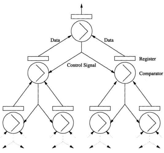
The hardware structure that implements the merge sort is a binary tree of comparator elements of depth log N, N being the number of elements to compare. The leaves of the tree each contain a single element of the data set that is to be sorted. Each node of the tree performs a comparison of its two inputs from its subnodes, stores the higher value in a register which is connected to the output of the node, and then tells the subnode that had the higher value to load a new value into its register. The subnode that gets the load signal performs the same operation, and so on, until a leaf node is hit. After log N cycles, the largest value is available from the top node, and another value is available on each subsequent clock cycle until the complete sorted list has been output. Figure 3.1 shows a graphical representation of the merge sort hardware construct.

Figure 3.1 Merge Sort Hardware Construct

Performance Results

The data presented here assumes that the internal virtual wires clock is 25MHz. Also, any cycles devoted to /10 between the host and the emulation system is also not included in the results. Only cycles dedicated to actual computation are included in the performance measures. In other words, the cycles required to load data into and to read results from the computation structures are not included.

Results

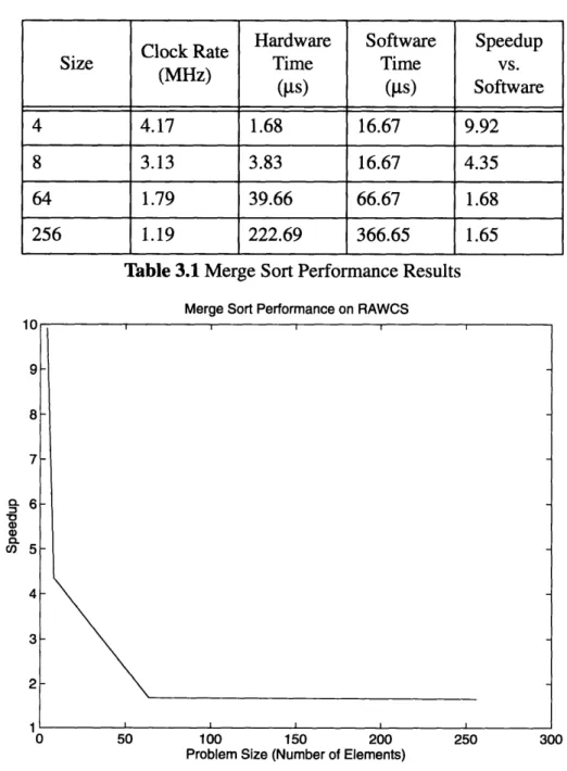
Unfortunately, the merge sort on RAWCS exhibits only a constant speedup over the sequential C version and does not scale well to larger problem sizes. Table 3.1 shows the speedup that the RAWCS implementation of merge sort has over the sequential C version

___ __I_·_·____·_

for problem sizes of 4, 8, 64, and 256 elements. Notice that the speedup is substantial for the smallest problem size but seems to asymptotically reach a speedup of only 1.6 as the problem size increases. Figure 3.2 is a graphical representation of the data presented in Table 3.1

Hardware Software Speedup Clock Rate

Size Time Time vs.

(MHz) ((ts) (gs) Software 4 4.17 1.68 16.67 9.92 8 3.13 3.83 16.67 4.35 64 1.79 39.66 66.67 1.68 256 1.19 222.69 366.65 1.65

Table 3.1 Merge Sort Performance Results Merge Sort Performance on RAWCS

0 50 100 150 200 250

Problem Size (Number of Elements)

Figure 3.2 Merge Sort Performance Results

Analysis

The disappointing results of the merge sort probably indicate that there is some combinatorial path through the computation structures that is limiting the speed of the computation. This critical path probably comes from the control signals that higher nodes send to lower nodes to load a new value into their register. When the root of the tree sends a load signal, it must propagate all the way down the tree to some leaf node. Since any leaf node could be the final recipient of a root node load signal, every leaf node becomes the terminating end of a critical path. Since the root node and leaf nodes could be separated very far from each other, perhaps even on different boards of the system, this critical path could slow down the clocking rate of the system by a great deal especially as the problem size grows.

One way to alleviate the problem would be to limit the number of nodes in the system to correspond to the number of elements in the problem and to add a new control structure that multiplexed the nodes during the computation. In the current implementation, most of the nodes are idle at any one time, so multiplexing should not pose a significant scheduling problem. By limiting the number of nodes and multiplexing their use, similar to the software implementation, inter-node communication would be greatly reduced and should result in improved performance in both absolute terms and relative to increasing problem sizes.

Chapter 4

Travelling Salesperson Problem

4.1 Problem Description

The travelling salesperson problem (TSP) can informally be stated as:

A travelling salesperson is given a map of an area with several cities. For any two cities in the map, there is a cost associated which is associated with travelling between these two cities. The travelling salesperson needs to find a tour of minimum cost which passes through all the cities. [18]

Formally, the problem is modeled as an undirected weighted complete graph. There is a path from every city to every other city, and any path can be traversed in either direction. The vertices of the graph represent the individual cities, and the edge weights represent the distances between the cities.

For any cyclic ordered tour through the cities, there is an associated cost function which is simply the sum of the edges between each city pair in the tour. The TSP minimization problem is defined as follows:

Instances: The domain of instances is the set of all

undirected weighted complete graphs.

Solutions: A feasible solution for a graph is a permutation over its vertices.

Value: The value of a solution for the graph is the cost of the corresponding tour.[181

The TSP is NP-Complete which means that there is no known algorithm that can compute an optimal solution in polynomial time.

4.2 Algorithms for Finding a Solution

The TSP is one of the most studied problems in all of computer science because of its broad applicability to so many different applications such as scheduling and circuit

routing. As such there have been many methods developed to solve or approximate a solution.

Exhaustive Search

A brute force search through all of the possible paths given a graph of cities is, of course, the most simple and the most time consuming. An exhaustive search is guaranteed to find the optimal solution, but the number of paths to search are generally so large that even for very small problems, a large parallel machine is required to actually implement this algorithm. If N is the number of cities in the graph, there are (N-i)! total paths that must be searched. If there are just 50 cities, the corresponding number of paths to search is 6.08E+62!

Branch and Bound

This algorithm continually breaks up the set of all tours into smaller and smaller subsets and calculates a lower bound on the best possible tour that can arise from that subset. An optimal tour is found when there is a path that is shorter than all of the lower bounds of all the remaining subsets. This algorithm can be used to solve TSPs on the order of tens. Going beyond that limit is not actually feasible.[21][22]

Simulated Annealing

Simulated annealing is an approximation algorithm which maps well to solving large TSPs. The algorithm is designed to mimic physical processes where a system at a high energy state is made to come to rest at a desired equilibrium at a lower energy state. For example, consider the physical process of cooling a liquid. In order to achieve a very ordered crystalline structure in the solid state, the liquid must be cooled (annealed) very slowly in order to allow imperfect structures to readjust as energy is removed from the

system. The same principle can be applied to combinatorial minimization problems such as the TSP.[23]

Of course, simulated annealing is an approximation algorithm which means that, although there is a chance that it may find the actual optimal solution, that event is highly unlikely. However, for large TSPs, approximation algorithms are the only feasible solution, and simulated annealing has been shown to provide very good approximations for large problem sizes.

4.3 RAWCS Implementation

Although simulated annealing is only an approximation algorithm, it was chosen as the candidate for RAWCS implementation because of its wide applicability to many different problems. Any kind of optimization problem where an exact answer is not a necessity can utilize this algorithm. Furthermore, there are many opportunities to exploit parallelism in the algorithm as will be discussed later.

Software Design

The software to implement the simulating annealing is written in C and was compiled and executed on a Sun (Sun Microsystems Inc.) SPARCstation LX with 32 MB of memory.

The software assumes that the input is a Euclidean TSP in the plane that satisfies the triangle inequality. This simply means that the software assumes that the problem is a weighted fully connected undirected graph in a single plane where every three cities, A, B and C, satisfies the triangle equality. Satisfying the triangle equality simply means that the distance between any two cities, A and B, is shorter than the sum of the distances from A to B and from B to C.[18]

The software reads in a file containing cities and their respective X,Y coordinates. It then calculates all of the inter-city distances and stores these values in a matrix. After

calculating the minimum spanning tree (MST) for the fully connected, undirected graph, the software uses the MST to find an initial path through the cities. This initial ordering is then passed on to the annealing procedure.

The simulating annealing procedure is a huge loop within a loop. The outer loop is the temperature cooling schedule. When the temperature falls below the final temperature, the annealing ends, and the current tour is returned as a solution. In the inner loop, there are a maximum of 500 * N, N being the number of cities in the graph, iterations performed at each temperature. If there are ever more than 60 * N swaps that are accepted, either by the fact that they shorten the tour or are accepted probabilistically, at any temperature, then the inner loop is broken even though 500 * N swaps have not been tried.

To simulate annealing, the procedure chooses two cities at random, swaps them, and calculates the change energy caused by the swap. This involves only six distance queries into the inter-city distance matrix. If B and E are the two cities chosen at random to be swapped, and A is the previous city to B in the current tour, C is the city after B in the current tour, and similarly for D and F for E, then calculating the energy change involves adding the distances from A to E and from E to C and D to B and B to F (the new tour) and subtracting the distances from A to B and from B to C and D to E and E to F (the previous tour).

Once the energy change for a random swap has been computed, the swap is accepted if the energy change was negative meaning that the new tour is shorter with the swap. If the energy change is positive meaning that the new tour is actually longer with the swap, it is accepted with a certain probability. That probability is determined by calculating the following equation: -EnergyChange

When either 500 * N swaps have been attempted or 60 * N swaps have been accepted, the temperature is decreased and the inner loop repeats. The process continues until the temperature falls below the pre-specified final temperature, or there is an iteration where no swaps are accepted.

Hardware Design

The first step in implementing simulated annealing on RAWCS is to identify the inner loop that will be executed on the reconfigurable emulation system. The obvious choice is to place the entire simulated annealing loop on the VirtuaLogic System.

The goal of the first phase of the RAWCS hardware design for simulated annealing was to create computation structures that would implement the simulated annealing loop but would also provide a framework to exploit both coarse-grained and fine-grained parallelism by extending and augmenting that framework.

In this first phase, there are three modules that were created:

1. A distance matrix which holds all of the inter-city

distances. There is only one such matrix in the current implementation. A single distance request from each simulated annealing module is processed at each clock tick.

2. A simulated annealing module which actually performs the annealing. Each module works on its own private copy of a tour. At the end of annealing, the module with the shortest tour returns it as the solution.

3. A control module which controls the operation of the

simulated annealing modules. It provides the temperature cooling schedule and notifies the simulated annealing modules to return solutions when the temperature cools to below the threshold.

Exploiting Parallelism

Coarse-grained parallelism refers to how the interconnection of the various modules can be altered to exploit parallelism. Fine-grained parallelism refers to how the modules

themselves can be modified to exploit parallelism of the computations made within the modules.

Coarse-Grained

The first modification that could be done would be to have a global current tour that is operated on by all of the simulated annealing modules simultaneously. This would require locking mechanisms on such a global tour data structure so that no two simulated annealing modules will try to swap the same city to two different locations. Having a global tour would allow many more swaps to be attempted during the same execution time.

Another modification that could be made would be to have multiple distance matrices each with multiple ports. Currently, there is only one distance matrix that services a single request per simulated annealing module per clock tick. Having a matrix for each simulated annealing module that can handle six distance requests per clock tick would allow all of the inter-city distance queries to complete in a single tick. In RAWCS, it is a simple matter to create a memory or bank of registers with multiple ports to parallelize the accesses into the distance matrix. It is guaranteed, from the previous modification, that each of the six distance accesses will be unique, so there will be no contention for a memory location. Furthermore, the inter-city distance matrix does not change over time, so multiple simulated annealing modules having their own private multi-ported inter-city distance matrix would not pose any coherence problems.

Fine-Grained

In the main simulated annealing loop, there are three basic computations performed during computation:

1. Once the swap is chosen at random, multiple queries

E toC DtoB BtoF AtoB BtoC DtoE EtoF

Energy Change for Swap

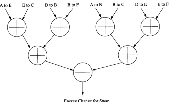
Figure 4.1 Parallelizing Energy Change Calculation

2. The energy change calculation is done based on the results of the queries into the distance matrix.

3. For swaps with positive energy change, calculation of the exponential is performed to see if the swap will be accepted anyway.

The energy change calculation can easily be parallelized in custom hardware to execute in O(log N) time, N being the number of terms in the summation, by using the hardware construct shown in Figure 4.1. The inputs are simply the distances between the respective cities where B and E are the cities to swap, A is the city before and C is the city after B in the current tour and, D is the city before and F is the city after E in the current tour.

Parallelizing the calculation of the exponential in determining acceptance of swaps with positive energy change is not possible. There is no opportunity to parallelize the calculation of an exponential. Furthermore, the use of floating point values in these calculations makes them extremely difficult to map to reconfigurable logic.

Chapter

5

Numerical Approximations for Simulated Annealing

5.1 Numerical Approximations

In order to implement the simulating annealing algorithm on reconfigurable hardware, all of the floating point operations must be converted to equivalent integer computations. This conversion must be done because the floating point operations in the implementation of the algorithm do not map well to reconfigurable hardware, nor do they offer any opportunities to exploit parallelism using custom hardware. This study is intended to answer the following question:

What effect does the conversion to integer approximations have on the simulated annealing algorithm in terms of

solution quality and computation time?

There are two floating point math operations that are at the heart of the simulated annealing algorithm. The first is the temperature cooling schedule, and the second is the calculation of the exponent in the probabilistic acceptance of a positive energy change.

Generally, the temperature cooling schedule is an exponential function with the initial temperature starting at a high value and decreasing by some fixed percentage at each iteration of the algorithm. To convert this schedule to the integer domain, a linear cooling schedule must be adopted.

A numerical approximation for the exponential function in the probabilistic acceptance of a positive energy change during the annealing is of the following form:

X = -energyChange

Temperature(T)

x X X

e = I+X+ +X +...

Given that X is an integer, this approximation can be completely done using integer values.

5.2

Data Sets

The data sets for the simulated annealing were created at random. A random number generator was used to create a random map of cities based on a parameter denoting how many cities the map should have.

Maps for 20, 80, 320, and 640 cities were created. These values were chosen in order to have two TSPs at the low end and two at the high end because it was assumed that conclusions about data sets in the middle could be inferred from the results based on these graphs. Refer to Appendix C for a graphical representation of the data sets.

5.3

Base Case

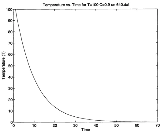
A base case had to be chosen as a metric to measure performance of all of the variations on the simulated annealing algorithm. The parameters for the base case were 100 for the initial temperature, a cooling rate of 0.9, a final temperature of 0.1, and the use of the exp function in the gcc math.h library to calculate the exponential in the probabilistic acceptance of positive energy changes.

An initial temperature of 100 was chosen because the way the city graphs were created, the energy changes from swaps were generally in the hundreds. Furthermore, at a cooling rate of 0.9, an initial temperature of 100 had 66 distinct temperatures before falling below the final temperature of 0.1. A maximum of 66 iterations seemed reasonable. A cooling rate of 0.9 and a final temperature of 0.1 were chosen for the same reasons.

Results

Figure 5.1 shows the temperature cooling schedule given the parameters for the base case. The graph is an exponential curve.

10( 9( 81 71 66 E I4 3 2 1

Temperature vs. Time for T=100 C=0.9 on 640.dat

Time

Figure 5.1 Temperature Cooling Schedule for Base Case

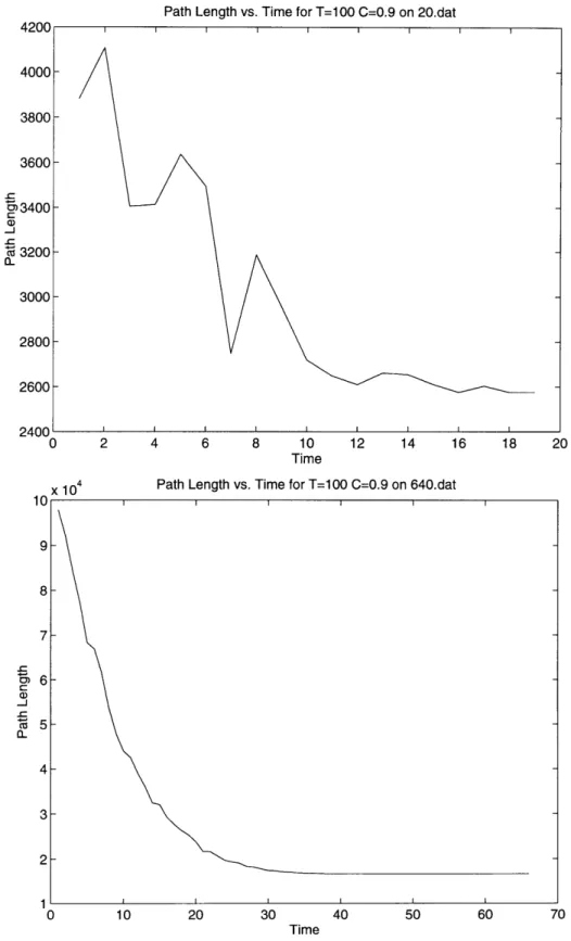
Figure 5.2 shows the path length for the current tour as the simulating annealing is performed on the 20 and 640 city TSPs. Notice that the path length is not always decreasing and that there are several points where the path length actually increases meaning that the probability function caused swaps with positive energy changes to be accepted. Notice how closely the path length improvements follow the cooling schedule especially in the 640 city problem.

Refer to Appendix D for a graphical representation of the TSP solutions that the base case found for the 80 and 640 city problems.

5.4 Linear Temperature Schedule

The first variable that was studied was the temperature cooling schedule. What effect does a linear temperature schedule have on the solution quality and time for computation of the simulated annealing?

4200 4000 3800 3600 --cn3400 c 3200 3000-2800 2600 24UU iv 9 8

Path Length vs. Time for T=100 C=0.9 on 20.dat

I I I I I I I

0 2 4 6 8 10 12 14 16 18 Time

x 104 Path Length vs. Time for T=100 C=0.9 on 640.dat

0 10 20 30 40 50 60 70

Time

Figure 5.2 Performance of Base Case on Two Problems

The restrictions on these experiments were that the parameters chosen had to ensure that the number of distinct temperatures possible during cooling had to be 66 which is the

- -- -- --

--i J i i i i i i

I

Temperature vs. Time for Linear Cooling Schedule 200 , T\=199, C=3 180 160 140 -S120 I 100 E ( 80 60 40 20 0 0 10 20 30 40 50 60 70 Time

Figure 5.3 Linear Cooling Schedules

same as the base case. This was to ensure that a new cooling schedule would not perform better or worse simply because it had more or less opportunity to find a better solution than the base case. Given that restriction, the initial temperature could also not deviate too far from the initial temperature of 100 in the base case. This was to insure that what was affecting the solution was not the magnitude of the temperature but the slope of the cooling schedule. Also, the gcc exp function was still used to calculate the exponential in the probabilistic acceptance function.

The parameters chosen for these experiments were initial temperatures of 67, 132 and 199 and cooling rates of 1, 2 and 3 respectively. These parameters fit the restrictions. No other set of parameters was really possible while staying within the restrictions.

Results

Figure 5.3 shows the linear cooling schedules for the three sets of parameters.

---Time to Find Best Length vs. Cooling Schedules 120( 1000 800 600 400 200 0.8 0.6 1 1.2 1.4 1.6 1.8 2 2.2 2.4 2.6 2.8

Linear Cooling Schedules

x 104 Best Length vs. Cooling Schedules

1.2 1.4 1.6 1.8 2 2.2

Linear Cooling Schedules 2.4 2.6 2.8 3 Figure 5.4 Performance of Linear Cooling Schedules

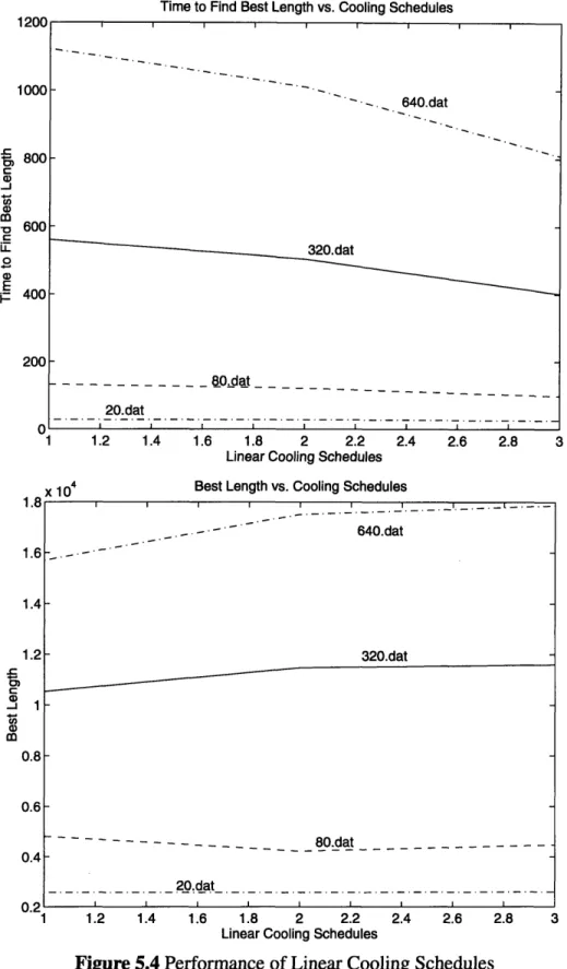
Figure 5.4 shows the performance of the three linear cooling schedules on the four

:) S. 640.dat 320.dat - _80.dat I I I I I I I I I `-· 640.dat 320.dat

---

--

80dat

problem sizes. The top graph shows how long it takes the three different schedules to complete their respective computations on the four randomly generated TSPs. On the y-axis, 1, 2 and 3 refer to initial temperatures of 67, 132 and 199 respectively. Notice that the initial temperature of 67 takes the longest time to compute and that the compute time decreases as you increase the initial temperature.

The bottom graphs shows the length of the optimal tour produced by each linear cooling schedule on the four randomly generated TSPs. Notice that as the initial temperature is increased, the length of the optimal tour found by simulated annealing increases.

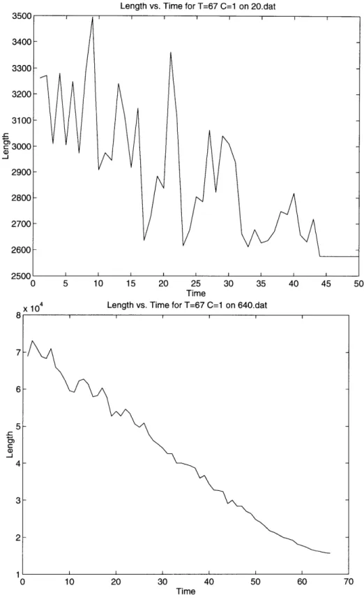
An initial temperature of 67 seems to produce the best answer among the three different schedules, albeit at a cost of longer computation time. Figure 5.5 shows the length of the current ordering during annealing of this best cooling schedule. The upper graph shows execution on the 20 city TSP. Notice how much more chaotic the path length is than the equivalent graph for the base case. The lower graph shows execution on the 640 city TSP. Again, notice how closely the path length during execution follows the linear cooling schedule.

Analysis

There is an obvious trade off in time vs. solution quality among the three linear cooling schedules. The lower the initial temperature, the better the solution quality but the longer the computation time. Why does this occur?

The higher the initial temperature, the greater the volatility in the annealing process which would tend to produce poorer results. With an exponential decay, a high initial temperature quickly drops away so that the effects of high temperatures on the probability function for positive energy changes is short-lived. However, with a linear decay, the

Length vs. Time for T=67 C=1 on 20.dat

0) -.

5 10 15 20 25 30 35

Time

Length vs. Time for T=67 C=1 on 640.dat

40 45 50

0 10 20 30 40 50 60 70

Time

Figure 5.5 Performance of Best Linear Schedule

temperature stays high much longer such that the volatility of the system is much greater. The total potential energy of the system can be equated with the area under the graph of

0

x 104

the cooling schedule, so that high initial temperatures have a magnified effect on the quality of the final solution thus leading to poorer solutions.

Also, at higher initial temperatures more swaps with positive changes in energy are accepted. Since the total number of swaps that are permitted per distinct temperature are limited by 60 * N, N being the number of cities in the problem, the higher initial temperature schedules hit this limit much more frequently for each distinct temperature than the lower temperature schedules. The lower temperature schedules must try many more swaps at each temperature because fewer positive swaps are probabilistically accepted.

5.5

Probability Approximation

The second variable studied was the calculation of the exponential in the probabilistic acceptance of swaps which actually increase the length of the current tour. What effect does an approximation for the exponential have on the solution quality and time for computation of the simulated annealing?

The parameters for these experiments were 1, 2, 3 and 4 terms in the following approximation equation for the exponential:

= -energyChange

Temperature(T) 2 3

e = 1+X+-•+-+... 2! 3!

1 term means a single X term was used in the approximation. The initial temperature was 100 and the standard exponential cooling schedule of 0.9 was used as in the base case. All other values were integers, and when temperature was used in a calculation, the result was cast to type int before being assigned to the variable.

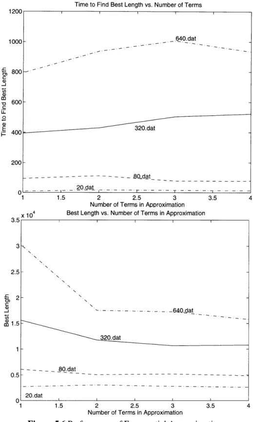
1200 1000 800 600 400 200

Time to Find Best Length vs. Number of Terms

-640.dat -·· -- --- 320.dat 20.dat -.-- I T-,- - - - -T -2 2.5 3

Number of Terms in Approximation

x 104

2.5

0.5

Best Length vs. Number of Terms in Approximation

2 2.5 3

Number of Terms in Approximation

Figure 5.6 Performance of Exponential Approximation

Results

Figure 5.6 shows the performance for the four approximations for the four problem

48 --- 640,dat

320.dat

sizes. The Y-axis indicates the number of terms used in the approximation. The upper graph shows the time for computation. Generally, increasing the number of terms increases the computation time since there are simply more calculations to perform when the swap has positive energy change.

The lower graph shows the length of the shortest tour found by each approximation on the four problem sizes. Notice the huge increase in solution quality, especially for the large TSP, when the approximation goes from 1 term to 2. Unfortunately, this huge jump causes the other improvements to seem small due to the scaling of the Y-axis, but the improvement in solution quality as the number of terms in the approximation is increased is quite appreciable.

Figure 5.7 shows the length during execution of the 4 term approximation on the 20 and 640 city TSPs. Notice how similar these graphs are to the corresponding graphs for the base case.

Analysis

The 4 term approximation provides the best solution quality but also runs the slowest because it simply has more computations to perform than the approximations with fewer terms. This is not a surprising result.

5.6

Finding the Best Numerical Approximation

The best numerical approximation should arise from combining the linear cooling schedule and the exponential approximation which gave the shortest path tours. The best linear cooling schedule was an initial temperature of 67 and a cooling rate of 1. Four terms in the approximation gave the shortest path.

Best Length vs. Time for 4 Term Approximation on 20 Cities

Time

x 104 Best Length vs. Time for 4 Term Approximation on 640 Cities

10 20 30 40 50

10 20 30 40 50

Time

Figure 5.7 Performance of Best Approximation

10

f%^^

Best Length vs. Problem Size

100 200 300 400 500 600 700

Problem Size

Time to Find Best Length vs. Problem Size

100 200 300 400 500

Problem Size 600 700 Figure 5.8 Performance of Best Numerical Approximation

Results

Figure 5.8 shows the shortest path found for all four problem sizes for both the base

x104 Standard . T=67, C=1, 4 Terms I I I I I I 1.6 1.4 0.6 0.4 0. 0 0 I 0VV 1200 1000 800 600 200 T=67, C=1, 4 Termsa Standard I -1~ -E H 02n ~n· -E

case and the complete numerical approximation using an initial temperature of 67, a linear cooling rate of 1, and four terms in the approximation for the exponential. The numerical approximation actually finds better solutions than the base case, but it takes longer to execute. The difference in solution quality grows with the problem size, but so does the computation time. As a matter of fact, the difference in computation time seems to grow

faster than the improvements in solution quality.

By increasing the slope of the temperature cooling schedule, there should be a corresponding decline in both solution quality and time for computation. Figure 5.9 shows the shortest path found for all four problem sizes for both the base case and the complete numerical approximation using an initial temperature of 132, a linear cooling rate of 2, and four terms in the approximation for the exponential. The numerical approximation almost exactly mimics the solution quality given by the base case, and it also performs slightly better in terms of computation time.

Analysis

As can be seen from the results, the complete numerical approximations work just as well or better than the floating point base case.

1.8 1.6 1.4 1.2 0.8 0.6 0.4 0 1200 1000

Best Length vs. Problem Size

100 200 300 400 500 600 700

Problem Size

Time to Find Best Length vs. Problem Size

800 600 400 200 0 0 100 200 300 400 Problem Size 500 600 700

Figure 5.9 Improved Computation Time

T=132, C=2, 4 Terms Standard Standard T=132, C=2, 4 Terms x 104 r ~

-Chapter 6

Conclusions

6.1 Merge Sort

The merge sort algorithm has been successfully implemented using RAWCS. Unfortunately, the implementation only exhibits a constant speedup over execution on a traditional workstation. This lack of performance gain is probably due to a critical communication path in the hardware that is slowing the emulation clock rate.

The RAWCS merge sort implementation shows that a compiler for a reconfigurable computer must do several things. First, such a compiler must be able to glean all of the possible parallelism out of the application in order to make the use of reconfigurable resources worthwhile. Even ignoring I/O limitations, reconfigurable hardware will never be clocked as fast as a microprocessor, so exploiting parallelism is the only way to make the use of reconfigurable hardware feasible.

Second, synthesizing for FPGAs is an extremely long and arduous task. Even on the fastest workstations, completely synthesizing a design takes on the order of days to complete. So, as in merge sort, a compiler for a reconfigurable computer must focus on generating hardware modules which can simply be replicated for larger problem sizes in order to cut down on synthesis time. Then, once a single module is synthesized, making copies of that same module simply involves placement and routing without the need to re-synthesize that module. If a compiler generated many unique elements, then the synthesis time, even assuming future improvements in the synthesis software, may negate the performance gains that reconfigurable computers offer.

Finally, a compiler for a reconfigurable computer must take communication requirements into careful consideration when implementing hardware constructs for an

application. The RAWCS merge sort implementation attempted to exploit parallelism without regard to efficient use of the generated hardware or the communication requirements that such a large collection of modules would require. Intelligent multiplexing of hardware must be at the heart of any compiler for a reconfigurable computer in order to minimize inter-module communication and also to minimize reconfigurable hardware utilization which is generally at a premium and limited on a reconfigurable computer.

Refer to Appendix A for the source code for the merge sort implementation using RAWCS.

6.2 TSP

A basic implementation of the simulated annealing algorithm has been written but has not been compiled or simulated. During development, it was discovered that the temperature cooling schedule and the calculation of the exponential in the probabilistic acceptance swaps with positive energy change could not be mapped to reconfigurable hardware.

Therefore, experiments were conducted to study the effects of using only integer values for all data and approximations for the exponential. It was found that these changes had no noticeable effect on the solution quality of the algorithm which means that the inner loop of the simulated annealing solution to the travelling salesperson problem should map well to RAWCS which, in turn, should be able to take full advantage of the fine-grained parallelism in the approximated version. The custom hardware to implement the exponential function in parallel is shown in Figure 6.1. In addition, parallelizing the distance accesses and energy change calculation, as shown before, should give the simulated annealing algorithm good speedup with RAWCS over the sequential implementation.

Solution

Figure 6.1 Parallel Implementation of Exponential Approximation

The implementation of the simulated annealing algorithm shows that a compiler for a reconfigurable system must be capable of making the same kinds of approximations automatically. Whether it is complex math functions, as in simulated annealing, or some other functions that do not map well to reconfigurable hardware, the compiler must recognize those opportunities where an approximation will suffice instead of throwing up its hands and saying that it is impossible to use the reconfigurable resource to implement a particular problem.

Refer to Appendix B for the source code for the TSP implementation on RAWCS.

The RAW Compiler

The work presented here only touches the tip of the iceberg in terms of the analytical ability and complexity that a compiler for a reconfigurable computer must have. Essentially, a compiler for such a system must automatically do many of the things that an experienced hardware designer must do. It must have the ability to find and create hardware to exploit parallelism in applications keeping in mind hardware efficiency and communication minimization. The compiler must also recognize and formulate