Data-driven approximation algorithms for rapid performance evaluation and optimization of civil structures

performance evaluation and optimization of civil structures

The MIT Faculty has made this article openly available.

Please share

how this access benefits you. Your story matters.

Citation

Tseranidis, Stavros, Nathan C. Brown, and Caitlin T. Mueller.

“Data-Driven Approximation Algorithms for Rapid Performance Evaluation

and Optimization of Civil Structures.” Automation in Construction 72

(December 2016): 279–293.

As Published

http://dx.doi.org/10.1016/j.autcon.2016.02.002

Publisher

Elsevier

Version

Author's final manuscript

Citable link

http://hdl.handle.net/1721.1/119411

Terms of Use

Creative Commons Attribution-NonCommercial-NoDerivs License

Automation in Construction

Data-Driven Approximation Algorithms for Rapid Performance Evaluation

and Optimization of Civil Structures

Stavros Tseranidis a_{, Nathan C. Brown} a_{, Caitlin T. Mueller}a,*

a _{Massachusetts Institute of Technology, Building Technology Program, Department of Architecture, Cambridge, MA 02139, USA}

* _{Corresponding author. Address: 77 Massachusetts Avenue, Room 5-418, Cambridge, MA 02139, USA. Tel. +1 617 324 6236. Email address:}

caitlinm@mit.edu (C. Mueller)

Abstract

This paper explores the use of data-driven approximation algorithms, often called surrogate modelling, in the early-stage design of structures. The use of surrogate models to rapidly evaluate design performance can lead to a more in-depth exploration of a design space reduce computational time of optimization algorithms. While this approach has been widely developed and used in related disciplines such as aerospace engineering, there are few examples of its application in civil engineering. This paper focuses on the general use of surrogate modelling in the design of civil structures, and examines six model types that span a wide range of characteristics. Original contributions include novel metrics and visualization techniques for understanding model error, and a new robustness framework that accounts for variability in model comparison. These concepts are applied to a multi-objective case study of an airport terminal design that considers both structural material volume and operational energy consumption.

Key Words: surrogate modelling, machine learning, approximation, structural design

1. Introduction

The engineering design process for civil structures often requires computationally expensive analysis and simulation runs within a limited timeframe. When the assessment of a design’s performance takes hours or days, the potential for exploring many solutions and significantly improving design quality is limited. This paper addresses this issue by investigating the application of surrogate modelling, a data-driven approximation technique, to civil engineering, to empower designers to achieve more efficient and innovative solutions through rapid performance evaluation.

1.1 Design optimization for civil structures

An established method for high-performance engineering design is optimization. However, unlike in other engineering disciplines, the optimization objectives and constraints in civil and architectural structures, such as buildings and bridges, are not always easily quantified and expressed in equations, but rather require human intuition and initiative to materialize. For this reason, design optimization in civil engineering has yet to reach its full potential. There are a few examples where it has been successfully applied to buildings, such as in braced frame systems for tall buildings by Skidmore, Owings & Merrill (SOM) [1], but these cases remain exceptional. To illustrate the breadth of designs for braced frame systems such those in [1], a somewhat irregular design by Neil M. Denari Architects (High Line 23, New York City [2]) could be considered. While this design is not structurally optimized, its architectural success is closely linked to its structural system and geometry. Thus, in design optimization for buildings, there needs to be a balance between quantitative and qualitative objectives.

Both quantitative and qualitative goals pose challenges for the use of optimization in terms of computational speed. First, simulations such as structural analysis and predictions of building energy consumption often require significant computational power, increasing with the complexity and size of the project. Thus, optimization algorithms can usually require substantial execution time, slowing down or impeding the design process. On the other hand, because of the qualitative nature of civil engineering design with the hard-to-quantify considerations as described above, many iterations are required and the result is never likely to come up from a single optimization run. In practice, the combination of slow simulation and problem formulation challenges means that optimization is

rarely used in the design of architectural and civil structures. In fact, even quantitatively comparing several design alternatives can be too time-consuming, resulting in poor exploration of the design space and likely a poorly performing design.

1.2 Need for computational speed

The exploration of the design problem and various optimal solutions should ideally happen in real time, so that the designer is more productive. Research has shown that rapid response time can result in significant productivity and economic gains [3]. The upper threshold for computer response time for optimal productivity has been estimated at 400ms and is commonly referred to as the Doherty threshold [3]. This threshold was originally developed in the 1980s for system response of routine tasks, like typing. Today, however, software users expect similarly rapid response for any interactions with the computer, even those that require expensive calculations like performance simulation. Immediate response from the computer can benefit not just rote productivity, but also creative thinking. The concept of flow is used in cognitive science to describe “completely focused motivation,” when a person becomes fully immersed in a task, at their most productive and mentally engaged. Among the key requirements for achieving creative flow, as, characterized by Csikszentmihalyi [4], is “immediate feedback”.

The first way to implement the “immediate feedback” effect in computer response is by increasing the available computational power. This can be achieved by either increasing the processing power of a computer or by harnessing parallel and distributed computing capabilities. The second way is to use different or improved algorithms. This paper focuses on the second approach, investigating algorithms that improve computational speed for design-oriented simulation through approximation.

1.3 Surrogate modelling

Among possible approximation algorithms, this paper considers surrogate modelling algorithms, a class of machine learning algorithms, and their use in making computation faster and allowing for more productive exploration and optimization in the design of buildings. Machine learning typically deals with creating models about the physical world based only on available data. The data are either gathered though physical experiments and processes, or by computer-generated samples. Those samples are then fit to an approximation mathematical model, which can then be used directly as the generating means of new representative data samples. In surrogate modelling specifically, the data is collected from simulations run on the computer.

Similar techniques are being used successfully in many other engineering disciplines, but have not been studied and applied extensively to the civil and architectural engineering fields. This research investigates these techniques and evaluates them on various related case studies. Focus is given in the development of a holistic framework that is generalizable. Figure 1 displays a core concept in surrogate modelling. The circles represent the available data, with many different models being able to fit them. The art in surrogate modelling is to choose the one that will also fit new data well.

1.4 Big data approach

The surge of available information is reshaping the existing methodologies in several scientific and engineering fields. It has been argued that the methodologies should take a shift towards data-driven approaches. As described by Denning [5], engineers can build algorithms that can “recognize or predict patterns in data without understanding the meaning of the patterns”. Furthermore, Mayer-Schönberger and Cukier [6] analyze this shift from causality to correlation in the methodologies in the “Big Data” era. Therefore, the term big data extends beyond the generation and accumulation of large amounts of data, to describe a new methodological paradigm based purely on data. Along these lines, this paper presents a data-driven approach for the design exploration of architectural and civil structures.

1.5 Organization of paper

First, a literature review of the existing research in surrogate modelling, its application in structural engineering problems, model types, and error assessment methods is outlined in Section 2. Section 3 is an overview of the main features of the methodology framework used, including assumptions and the models used. Sampling and normalization techniques are also discussed. Section 4 is dedicated to explaining the new error assessment and visualization methods used throughout the rest of the paper. Section 5 introduces the proposed method for robust model comparison, whose use is then illustrated through the case study in Section 6. Specifically, Section 6

introduces the case study problem, the parameters examined and the analysis assumptions, while also presenting all the numerical results obtained from the approximation. The original contributions, findings and future considerations are summarized in Section 7.

2. Literature review

To avoid a computationally expensive simulation, one approach is to construct a physical model that is simpler and includes more assumptions than the original. This process is very difficult to automate and generalize and requires a high level of expertise and experience in the respective field. A more general approach is to substitute the analytical simulation with an approximate model (surrogate) that is constructed based purely on data. This approach is referred to as data-driven or black-box simulation. The reason is that the constructed approximation model is invariant to the inner details of the actual simulation and analysis. The model has only “seen” data samples that have resulted from an “unknown” process, thus the name black-box. This paper addresses data-driven surrogate modelling.

The two main areas in which surrogate modelling can be applied are for optimization and design space exploration. Specifically, an approximation (surrogate) model can be constructed as the main evaluation function for an optimization routine or just in order to explore a certain design space in its entirety, better understand variable trade-offs and performance sensitivity. For optimization, it is often used when there are more than one optimization objectives, thus called multi-objective optimization (MOO), and the computational cost of computing them is significant.

2.1 Surrogate modelling for structural designs

In previous decades, when computational power was significantly less than that of today, scientists started to explore the possibility of adapting approximation model techniques in intensive engineering problems. One of the first attempts of this kind in the field of structural engineering by Schmit and Miura [7] in a NASA report in 1976. A review of the application of approximation methods in structural engineering was published by Barthelemy and Haftka in 1993 [8]. The methods explored in this review paper are response surface methodology (RSM) as well as neural networks (NN). It was mentioned that more methods will emerge and the practice is going to expand. In fact, today, although the computational power has increased exponentially from twenty years ago, the engineering problems that designers face have also increased dramatically in scale and therefore surrogate modelling has been studied and applied extensively.

In 1992, Hajela and Berke [9] contributed an overview of the use of neural networks in structural engineering problems. They noted that this approximation technique could be useful in the more rapid evaluation of simulations such as nonlinear structural analysis. Neural networks and approximation models more broadly still have great potential in this field today, when nonlinear structural analysis is very frequently performed. Researchers have been using approximation algorithms in the structural engineering field for various problems such as for the dynamic properties and response evaluation and optimization of structures [10], for seismic risk assessment [11] and for energy MOO simulations [12]. Energy simulations are extensively examined in this paper, since they are usually extremely expensive computationally, and at the same time their use and importance in building and infrastructure design is increasing today.

The use of approximation algorithms in conceptual structural and architectural design was examined by Swift and Batill in 1991 [13]. Specifically, for truss problems, with the variables being the positions of some nodes of the truss and the objective the structural weight, a design space was sampled and later approximated using neural networks.

A similar approach was followed by Mueller [14], with a seven-bar truss problem examined being shown in Figure 3a. The variables were again the positions of the nodes and specifically the vertical nodal positions as shown along with their ranges in Figure 3a. The design space (with the structural weight as the objective score) computed analytically, without approximation is shown in Figure 3b. The approximated design space for different models is shown in Figure 3. Details on the approximation models used later are presented in Section 2.2.

It is also noteworthy that surrogate modelling is used extensively in the aerospace industry. The basic principles remain the same across disciplines since the methodology relies solely on data. Queipo et al. [15] have made a thorough overview of the common practices of surrogate modelling. They also applied those techniques in an MOO problem from the aerospace industry. Another comprehensive survey of black-box approximation method for use in high-dimensional design problems is included in [16].

There exist attempts of integrating performance evaluation into parametric design in architectural and civil structures. Mueller and Ochsendorf [17] considered an evolutionary design space exploration, Shi and Wang [18] examined performance-driven design from an architect’s perspective, while Granadeiro et al. [19] studied the integration of energy simulations into early-stage building design. All of these interesting approaches could benefit by the use of surrogate modelling, which is the main contribution of this paper.

2.2 Model types

Several methods have been developed over the years to approximate data and have been used in surrogate modelling applications. Very common ones include polynomial regression (PRG) and response surface methodology (RSM) [20], in which a polynomial function is fitted to a dataset using least squares regression. This method has been used in many engineering problems [15].

One of the most widely used surrogate modelling method in engineering problems is Kriging (KRIG). Since it was formally established in the form it is used today [21], it has been applied extensively ([11], [15], [22]). Gano et al. [23] compared Kriging with 2nd order polynomial regression. Chung and Alonso [22] also compared 2nd order RSM and Kriging for an aerospace case study and concluded that both models performed well and are pose indeed a realistic methodology for engineering design.

Another very popular model type are artificial neural networks (referred as NN in this paper). Extensive research has been performed on this type of model ( [9], [15] ). Neural networks are greatly customizable and their parameters and architecture are very problem specific.

A special type of neural network is called radial basis function network (RBFN) and was introduced by Broomhead and Lowe [24] in 1988. In this network, the activation function of each neuron is replaced by a gaussian bell curve function. A special type of RBFN imposes the Gaussian radial basis function weights such that the networks fits the given data with zero error. This is referred to as radial basis function network exact (RBFNE) and its main drawback is the high possibility that the network will not generalize well on new data. Those two types of models, RBFN and RBFNE, are explained in more detail in Section 3 as they are studied more extensively in this paper.

Radial basis functions can also be used to fit high dimensional surfaces from given data. This model type is called RBF [25] and is different from the RBFN model. RBF models can also be referred to as gaussian radial basis function models [15]. Kriging is similar to RBF, but it allows more flexibility in the parameters.

Multivariate adaptive regression splines (MARS) is another type of model. This performs a piecewise linear or cubic multidimensional fit to a certain dataset [26]. It can be more flexible and capture more complex datasets, but requires more time to construct.

Jin et al. [27] performed a model comparison for polynomial regression, Kriging, MARS and RBF models. They used 13 mathematical problems and 1 engineering problem to perform the comparisons. Many other references for papers that performed comparisons between those and other models are also included in [27]. An important contribution of this paper was a list of five major aspects to compare the models: accuracy, robustness (ability to make predictions for problems of different sizes and type), efficiency (computational time to construct model), transparency (ability of the model to provide information about variable contribution and interaction) and conceptual simplicity. Those issues are examined in following sections in the present paper.

Finally, the existing MATLAB-based framework called SUMO [28], implements support vector machines (SVM) [29] (a model type frequently used for classification), Kriging and neural network models, along with the sampling and has been used in many applications such as RF circuit modelling and aerodynamic modelling [28].

A framework with NN, Random Forests (RF) (which have not extensively been applied in structural engineering problems), RBFN, RBFNE, MARS and KRIG models is developed and tested in case study problems in this paper to extend the existing research and available methodologies for structural design. There is a lack of extensive model comparison and their application on problems for structural engineering and building design specifically; this paper addresses this need to move beyond existing work.

2.3 Error in surrogate models

The most important error required to assess an approximation model is called its generalization error. This is more thoroughly examined in Section 2.4. In the current section, ways to quantify a model’s performance on a given set of data are discussed. When the actual performance calculated from the analytical simulation is known for a set

of data, and the respective performance from an approximation model is calculated, then the error of the predicted versus the actual performance can be calculated by many different measures. All the following error measures are computed between the actual (represented by y) – and predicted (represented by h) values.

One of the most common ones is R2_{, which refers to the correlation coefficient of the actual with the predicted}

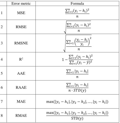
values. A value closer to 1 indicates better fit. This is extensively discussed in this paper in Section 4. Other common measures are the Mean Squared Error (MSE) and its root, the Root Mean Squared Error (RMSE). The Root Mean Square Normalized Error would be another alternative. It is more intuitive and more details are included in Section 4.2. The Average Absolute Error (AAE) and the Maximum Absolute Error (MAE) are other options, along with Relative Average Absolute Error (RAAE) and the Relative Maximum Absolute Error (RMAE). MAE is generally not correlated with R2 _{or AAE and it can indicate whether the model does not perform well only in a}

certain region. The same holds true for RMAE, which is not necessarily correlated with R2 _{or RAAE. However, R}2_,

RAAE and MSE are usually highly correlated [27], which makes the use of more than one of them somewhat redundant. Gano et al. [23] used R2_{, AAE and MAE for the model comparisons they studied, while Jin et al. [27]}

used R2_{, RAAE and RMAE. The above mentioned error metrics are summarized along with their formulas on Table}

1.

Error metric

Formula

1

MSE

∑

(𝑦

− ℎ

)

𝑛

2

RMSE

√

∑

(𝑦

− ℎ

)

𝑛

3

RMSNE

√∑

(

𝑦

𝑦

− ℎ

)

𝑛

4

R

_{1 −}

∑

(𝑦

− ℎ

)

∑

(𝑦

− 𝑦̅)

5

AAE

∑

|𝑦

− ℎ

|

𝑛

6

RAAE

∑

|𝑦

− ℎ

|

𝑛 ∙ 𝑆𝑇𝐷(𝑦)

7

MAE

max⁡(|𝑦

− ℎ

|, |𝑦

− ℎ

|, … , |𝑦

− ℎ

|)

8

RMAE

max⁡(|𝑦

− ℎ

|, |𝑦

− ℎ

|, … , |𝑦

− ℎ

|)

STD(y)

Table 1:Common surrogate modelling error metrics (y: actual, h: predicted value)

Error measures which provide a more direct and comprehensive quantitative model performance metric are lacking, and some alternative approaches to address this are presented in this paper. Error measures based on a model’s performance on the rank of the samples [14] are also studied. Special focus is also given to the visualization of the results and it is argued that normalization and visualization can have a significant impact in understanding error and are problem specific.

2.4 Robustness in surrogate modelling

As mentioned above, it is crucial for a surrogate modelling application to have an acceptable generalization error. This refers to an error estimate of the model on new data. In this context, new data means data samples that have not been used at any point in the construction of the model. One can realize that this is indeed the most important error required since the rapid generation of accurate new data performance is the main objective of the construction of the surrogate model in the first place.

To estimate the generalization error, several techniques exist. Those are explained in detail in Queipo et al. [15] and Viana et al. [30]. The simplest one is to split a given dataset into train and test data, construct the model with the train data and then compute the error in the test data and take this as an estimate of the generalization error. Another technique is called cross-validation (CV), in which the original dataset is split into k parts and the model is trained with all the parts except one, which is used as the test set of the previous case. The procedure is then repeated until each one of the k sets has served as the test set. By taking the mean of the test set errors, a more robust generalization error estimate is produced. Another advantage is that a measure of this error’s variability can be obtained by taking, for example, the standard deviation of the computed k test set errors. If this procedure is repeated the same number of times as the number of samples in the original dataset, which means that only a single sample is used every time as the test set, then this measure is called PRESS and the method leave-one-out cross validation [30]. The last method to obtain a robust generalization error measurement is through bootstrapping. According to the known definition of the bootstrap (sample with replacement), a certain number of bootstrap samples (datasets) are created as training and test sets. Then the error estimate and its variability calculation procedure is similar to the CV method. For the bootstrapping method to produce accurate results, a large number of subsamples is usually needed [30].

This paper attempts a combination of the aforementioned techniques frequently used in the surrogate modelling context with the common practice of machine learning applications (train/validation/test set partition) to obtain a measure of robustness as well as accuracy.

Another way to interpret robustness is to consider it as the capability of the approximation model to provide accurate fits for different problems. This again can be measured by the variance of accuracy and error metrics. However, the scope of this paper is to examine the deployment of approximation models for case study design problems and not to comment on a model’s more general predictive ability regarding its mathematical properties.

Finally, to increase robustness, one could use ensembles of surrogate models in prediction [15]. This means that several models are trained and their results are averaged with a certain scheme to obtain a prediction. Models of this type are Random Forests (RF), which are studied in this paper and explained in more detail in the next section.

3. Methodology and framework

This section outlines in detail the basic components used throughout this research, the proposed methodology and the case studies, all explained in the following sections. In general, the framework developed is based on first sampling a design space, and then constructing and assessing the surrogate models. For the sampling part, the Rhino software [31] and the Grasshopper plugin [32] were used. They are parametric design tools very broadly used in architectural design. As for the surrogate modelling part, the framework and all of the analysis was performed in MATLAB. References to the specific functions and special capabilities of MATLAB are placed in context in the text.

3.1 Surrogate modelling procedure

The basic surrogate modelling procedure consists of three phases; training, validation, and testing. A separate set of data is needed for each of those phases. During the training phase, a model is fit into a specific set of data, the training set. The fitting process refers to the construction of the mathematical model; the determination of various weighting factors and coefficients. In the next phase, the trained model is used on a different set of data, the validation set, and its prediction error on this set is computed. The first two steps of training and validation are repeated several times with different model parameters. The model that produced the minimum error on the validation set, is then chosen for the final phase of testing. During testing, another dataset, the test set, is used to assess the performance of the model chosen from the first two steps (minimum validation set error).

The steps are shown schematically in Figure 4. Each model type can have multiple parameters which define it. These are referred to as nuisance parameters, since they must be selected by trial and error in the validation step, or simply parameters in the following sections. Different nuisance parameters can result in different levels of model fit and accuracy. Choosing the best nuisance parameters for a given model type is the goal of the validation phase as described in the previous paragraph. The test phase is for verification of the model’s performance on a new set of data, never previously used in the process (training or validation). More details can be found in [29].

3.2 Model types

A surrogate model is essentially a procedure that acts on input data and outputs a prediction of a physical quantity. Previously computed or measured values of the physical quantity at hand, along with the corresponding input variables, are used to create/train the model, which can afterwards be used to make rapid predictions on new data. There are numerous different surrogate modelling algorithms and architectures. In the following section, the models examined in the present paper are introduced. Lists of the considered parameters affecting each model are also included. All the model parameters considered and MATLAB functions used are summarized in Table 2.

NN

RF

1

Number of neurons

6:6:30

Number of trees

10:10:300

2

Number of layers

1:2

Number of variables to sample

6

3

Training function

trainlm

Bootstrap sample size ratio

0.8

4

Maximum validation checks

10

Sample with replacement

true

5

Internal ratio of Training data

0.8

Minimum leaf observations

5

6

Internal ratio of Validation data

0.2

7

Internal ratio of Test data

0

MATLAB

feedforwardnet [33]

TreeBagger [34]

RBFN

RBFNE

1

Mean squared error goal

0.005

Spread of radial basis functions

0.5:0.5:4

2

Spread of radial basis functions 0.5:0.5:4

3

Maximum number of neurons

600

MATLAB

newrb [35]

newrbe [36]

MARS

KRIG

1

Piecewise function type

{cubic,

linear}

Degree of polynomial regression

function

{0,1,2}

2

Maximum number of functions

10:10:40 Correlation function

{exponential,

gaussian,

linear,

spherical,

spline}

MATLAB

ARES Lab [37]

DACE Toolbox [38]

Table 2:Summary of models, nuisance parameters and MATLAB functions considered

The first step of any surrogate modelling framework is sampling. It refers to the gathering of a finite number of samples of design space parameters (explanatory variables) with the corresponding objective value (performance measure) for each of those samples. Those samples will be separated into training, validation, and test sets for the model development phase.

For the case study in the present paper, the Rhinoceros software [31] was used along with the Grasshopper plugin [32] to generate the parametric design models as well as the objectives. For this reason, a sampling tool was developed for Rhino/Grasshopper since the existing ones were not deemed satisfactory.

All datasets used to train and assess the models have been normalized. The normalization scheme used is to make each variable have mean 0 and standard deviation 1. In more detail, once a dataset has been created through simulation, before the partition into train/validation/test set, each input variable column and the output vector was reduced by its mean and then divided by its standard deviation. Normalization is important to bring all the variables in the same range and prevent assigning unrealistic importance and bias towards some variables.

To finally assess the performance of the models, the completely separated test set was used. In order to better comprehend the results and the effect of a model, it was decided to normalize the performance score values (the output for the models) in a manner that the best performing design in the sampled data receives a score of 1 and the rest scale accordingly. For example, a score of 2 performs two times worse than the best design in the test set.

3.4 Design example

A design example of a parametric seven bar truss is introduced here and is used in the following sections to illustrate the methodology concepts presented. The “initial” geometry of the problem is shown in Figure 5.

The variables of the problem are x1, x2, and x3 as shown (along with their bounds in Figure 5 [14]). This case

study is for research purposes and the methodology is intended for more complicated problems where the structural and energy analysis has significant computational needs.

The variables examined were the horizontal – x1 – and vertical – x2 – position of one node of the truss as shown

in Figure 5 and also the vertical – x3 – position of the node that lies in the axis of symmetry of truss. It should be

noted that the structure is constrained to be symmetric. The design space was sampled based on the three (3) nodal position variables and each design was analyzed for gravity loads (accounting for steel buckling as well, which enhances the nonlinear nature of the problem) and a performance score of the form ΣAiLi (where A is the required

cross sectional area and L the length of member i) was determined as the objective.

Using the developed Grasshopper sampling tool described above, data were collected to later fit approximation models from. In Figure 5b, 15 designs produced are shown. Each design has a performance score associated with it, which is used to train an approximation model.

4. Error and visualization

In this section, the crucial issues of visualizing a model’s performance and measuring its error are discussed. Several visualization techniques are described and are used in the case studies.

4.1 Understanding error and visualization

When an approximation model is developed, the goal is to make the model “learn” a specific physical process or numerical simulation and be able to make predictions. Therefore, the main evaluation metric of a model is how well it performs at making predictions on new data, or in other words, how well it generalizes. The test set has the role of “new” data in a way that it comprises pristine data that were not used at any point in the model’s development process (training/validation). The use of a completely separate test set as described before is a very sound way to assess a models performance. In most cases, a test set can be kept when there is an abundance of data at the beginning of the model development process. In case only a relatively small dataset is available (in practice 10-100) then there are techniques such as cross-validation and bootstrap validation to compute a model’s generalization error without a separate test set. For the present case studies, the size of the dataset was sufficient and it was decided to use a test set to assess a model’s performance.

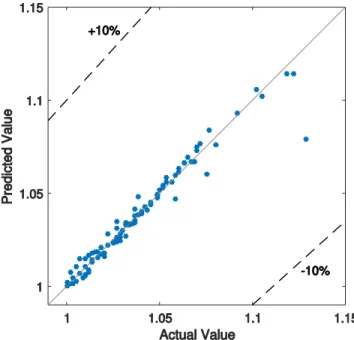
One of the most frequent ways to visualize a model’s performance is to scatter plot the actual values versus the predicted ones from the model (for either the training, validation or test set). In the perfect scenario where the model can perfectly predict the correct values, the points on this plot lie in a straight line with slope of 1 and the correlation

between actual and predicted values is 1. This type of plot is used the current paper on the test set data. The more closely the points lie in the slope-1 line, the better the predictive ability of the model.

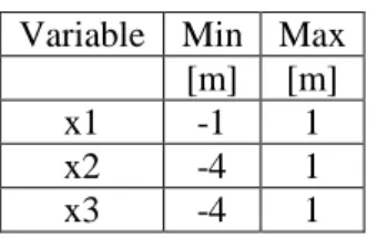
For the example case study of the seven bar truss as described in Figure 5 if we do a sampling in the range shown in Table 3 from the “initial” geometry, compute a structural score for each sample, partition in train/validation/test sets in 150/50/90 samples respectively and train models, we can assess them using the described scatter plot as seen in Figure 6 for an RBFN model with a spread of 2.5 (best validation set MSE).

Variable Min Max

[m]

[m]

x1

-1

1

x2

-4

1

x3

-4

1

Table 3: Seven-bar truss sampling ranges

A way to quantify the proximity of the points to the slope 1 line, the correlation of those two variables (Actual and Predicted performance) can be computed and the closer this value is to 1, the better the performance. This correlation metric is often referred to as the R-value in statistics. This scatter plot for the seven-bar truss problem for an RBFN model with spread 2.5 is shown in Figure 6. The two dashed lines represent the ±10% error ranges (this has been used in [11]).

As an extension to the scatter plot described previously, it is proposed to use scatter plots of each explanatory variable versus the score for both Actual and Predicted score to assess model performance. This plot is for the same RBFN model used previously as in Figure 6.

4.2 “Flat” model benchmark

Often it is difficult to comprehend a model’s performance in terms of MSE. This is because MSE is a single and somewhat abstract numerical value (possibly with a range). We can compare this value for different model types and across different nuisance parameters for the same model type, but there is lack of a physical intuition on what that number stands for on its own. Specifically, how can it be interpreted qualitatively in terms of the model making good predictions. One wonders how big or small this number is compared to the values of the scores, how does the normalization scheme affects it, if at all and other similar issues.

To address this, another scalar value for the error is needed to compare to, which is somehow internal to the data themselves without any model effect. One approach to obtain such a number would be to make a random model and calculate its error on the validation set. Specifically, make random predictions and calculate the error. It would be necessary to repeat this process a number of times to obtain an interval to which a t-test could be performed to determine whether a trained model has an effect on the predictions or it can be considered random.

A more simple approach that is proposed here and assists in a more rapid and qualitative evaluation of a model’s error is the “flat” model approach. This approach, instead of random predictions, considers a model that predicts a single value for each data point in a set. The proposed value is the arithmetic mean of the dataset. So, the model used to compute the error is a “flat” model that always outputs the same value as shown in Figure 8. It serves as a good benchmark (like the random prediction) since it does not reflect in any way the structure of the data and a surrogate model must surely have a considerably lower error than the “flat” model’s in order to be considered adequate.

For the seven bar truss example studied in the current section, the model comparison on the test set is shown in Figure 11a where the “flat” model error is the black dashed line at the top of the plot. The y-axis scale is logarithmic and we can observe that some models performed substantially better than the “flat” model, which is the desired effect. To further explain the “flat” model, the scatter plot produced for the test set is included in Figure 8. The predicted value is always the same (mean of Actual values); the “flat” model error is the MSE of the model represented in this scatter plot.

Finally, a different way to obtain an intuitive prediction error value would be to take the root of the mean square normalized error, with the formula shown as RMSNE in Table 1. This would be an error estimate of the percentage of the error on each sample entry.

5. Robustness

A robust model comparison methodology has been developed and is described in detail in this section. It was applied in several case study problems, with the results showcased in the next section. The motivation for this methodology is to have a way to quantitatively compare the performance of different families of models in approximating the same dataset. An important goal of the methodology is the extraction of an interval of a model’s error in addition to the average error value. The way to obtain this interval is not to make a single run of training models on a given train/validation set configuration, but use many configurations and make several runs. At first the structure of a single run is described. Then the process of generating more runs and aggregating them to compare the models is explained. This section introduces the main framework that has generated the results of the case studies.

5.1 Single run

In the first place, we assume that there is a single training set and a separate single validation set. A framework was developed in MATLAB to train all the six different types of models discussed here for different nuisance parameters for within each model type as well. The nuisance parameters considered for each model have been summarized in Table 2. The training set (the same for all the models) is first used to train the models. Then the mean squared error of those models is computed on the validation set (again the same for all models) and the nuisance parameters with the lowest error is chosen for each model type. This procedure is shown schematically on Figure 9, with the best nuisance parameter model chosen for each model type. One could then use the test set data, apply them to the best models and assess their performance through the visualization techniques described in the previous section.

5.2 Multiple runs

When a single run is carried out, a scalar is produced as the error of each model. However, the error resulting from the test depends in part on the specific data sets used for training and validation. The method proposed here seeks to characterize the effects of variability due to the data set so that the model’s general robustness can be understood. One method to obtain a variability measure for the error is cross-validation, which was described briefly in Section 3. In that section, it was also argued that when an abundance of data is available, it is preferred to choose a completely separate validation set and avoid cross validation. With those two facts considered; 1) abundance of data 2) a need for an error variability measure, a methodology of training the models for several different separated training and validation sets is proposed.

In detail, the aforementioned procedure for the single run is repeated for many different random partitions of the training and validation data pool. This means that the training and validation data are pooled and a certain number of random partitions of these data in training and validation sets with a constant number of samples in each set are generated. The validation set error (MSE) is stored for each different nuisance parameter and every model type. Afterwards, the mean of the MSE for each parameter across all partitions is calculated. Then the nuisance parameter with the minimum arithmetic mean MSE is chosen and the errors for this specific parameter for each partition are studied as the desired measure of the variability. The standard deviation is a metric that can be extracted from this information or just the range and the scatter can be examined. This process is applied for each model and the output is an error measure with the accompanying variability for each of the six models. For one model, the process is schematically shown in Figure 10. In this figure, there were five nuisance parameters considered and five different partition runs were carried out for each parameter. The errors are accumulated, with the thick dashed line showing the arithmetic mean of the runs for each parameter. The lowest-mean-error parameter was chosen; thick black box in the figure.

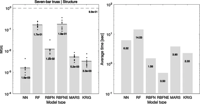
The results obtained after this process are summarized in a bar chart to compare the models, which was the original motivation. A bar chart for the seven-bar truss is included in Figure 11. The same chart is included in Section 7 where it is put in context. Each bar represents the mean of the error for each model type. The error of each run is also plotted in small black scatter dots to show the variability of the error. The number of the mean is also written inside each bar for easier reading of the whole graph.

A “Flat” model error measure was taken for the validation set for each partition and the mean is also plotted as a dashed straight line in the comparison bar chart, with the actual number also printed at the far right hand side of the line. The y-axis scale is in logarithmic scale to capture large differences in the results.

NN

RF

RBFN

RBFNE

MARS

KRIG

Mean

[%]

0.2

16.7

1.2

17.9

0.5

0.3

Max

[%]

0.4

25.7

3.4

36.6

0.9

0.8

Min

[%]

0.1

10.4

0.5

6.2

0.3

0.2

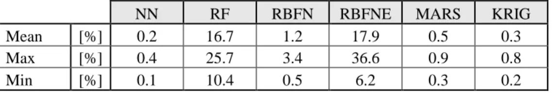
Table 4:Seven-bar truss model performance as per-cent of “flat” model error

From Figure 11, it can be observed that some models (NN, RBFN, MARS, and KRIG) performed very well, with RF and RBFNE performing the worst. The performance becomes more evident when someone looks at Table 4 which lists each models mean, maximum and minimum error as a percentage of the “flat” model error. The variability of each model’s performance can be visually inspected from the figure by looking at the black scattered dots representing the respective model’s error for each run. As another way to quantify the variability one can look at Table 5 which includes the percentage values of the maximum and minimum error with the respect to the mean one for each model, as well as the standard deviation of the runs’ errors.

NN

RF

RBFN

RBFNE

MARS

KRIG

Max

[% of

mean]

276

153

271

204

166

231

Min

[% of

mean]

33

62

41

34

56

55

St. Dev

-

0.001

0.048

0.008

0.095

0.002

0.002

Table 5:Seven-bar truss model error variability metrics

It is notable that NN has the lowest standard deviation, but has the largest Max value. This is observed from Figure 11, where there seems to be an outlier in the errors. This illustrates the reason that more partition runs are needed to increase the robustness of an error measure and make a better decision when choosing a model. Particularly, if only a single run was performed and it happened to be on this outlier set, then the eventual model selection could be different. These overlaps of the error metrics for different runs indicate that the model comparison picture could be different if the multiple runs and aggregation was not performed. This is very important, since it has a direct impact to the final model selection for the approximation in the project at hand.

Figure 11b shows a model construction time comparison bar chart. More specifically, it shows the average time needed to construct a model of each model type for a single run. It should be pointed out that this time includes the validation over several parameters and the eventual selection of the best parameters within each run; the procedure described in the first section of the current section for the “Single run”. It is notable that the best performing model in terms of error (NN) required the second longest time to build, while the worst performing (RBFNE) required the least time. And as mentioned before, this is mainly due to the fact that the NN iterates over more parameters and the best-performing network on the validation set is picked, while the RBFNE model only includes a single parameter (spread of the radial basis functions). The fact that the user can choose the number of parameter a model iterates over makes the picture even more complex. Overall, the trade-off between accuracy and time is evident from the above figures.

6. Case study

In this section, a case study of using the above-described surrogate modelling framework and new developments is presented. The problem description, the parameters considered, the performance scores and the finally the approximation fit and results are included in this section.

6.1 Problem description and parameters

The airport terminal design shown in Figure 13 is the focus of this case study. This design was inspired by an existing bus terminal shown in Figure 12. The terminal’s design was parametrized by 6 variables and included

various design objectives. The objectives were (1) the structural weight as described in the seven-bar truss design example (2) the total energy requirements including production and distribution losses (3) the cooling load of the structure as a building in an annual basis (4) the heating load (5) the lighting load and (6) the energy requirements as the sum of the cooling, heating and lighting loads.

The motivation for this case study is that both structural and energy simulations needed to assess design performance require substantial computational power; therefore, one cannot explore the design space in real time. This prevents the designer from fully comprehending the whole design space, realizing its full potential, or even rapidly run optimization routines over the selected variables. The use of surrogate modelling could replace the expensive simulation and allow for more deep exploration and optimization over the parameters.

The variables for this case study problem for which the structure was parametrized over are: x1, the horizontal

and x2, the vertical position of the cantilever, x3 the vertical position of the central node, with its horizontal position

always fixed in the middle of the two ground hinge supports. x4 and x5 represent the angles of the left and right side

respectively of the two truss members joining at the supports and x6 is the glazing ratio of the windows. The window

glazing ratio is important and can affect the energy related scores, since the energy simulation considers sunlight gains for both heating and lighting. Variable summary in Table 6.

Variable

Description

x1

Horizontal position of overhang tip

x2

Vertical position of overhang tip

x3

Vertical position of node on axis of symmetry

x4

Truss inclination 1

x5

Truss inclination 2

x6

Glazing ratio

Table 6:Airport terminal variables

6.2 Performance outputs

The simulation to measure the performance of each design sample was carried out in Rhino and Grasshopper plugins. For the structural performance, the objective was the structural weight and the simulation was performed using the Karamba plugin [40]. For all the energy simulations, the plugin ARCHSIM was used [41]. This plugin connects the parametric model from Rhino, to EnergyPlus [42], an energy analysis program available by the U.S. Department of Energy. More information about this problem, the setup and all the assumptions used in the simulations can be found on [39]. Each design evaluation required approximately 0.2 sec for the structure and 25 sec for the energy, making surrogate modelling an ideal solution.

Because this case study involved energy simulations, a lot of data were collected from simulating the same structure in different climates and orientations. The case study for NS orientation (longitudinal axis of Figure 13) is examined here.

Set

# samples

Training

600

Validation

200

Test

200

Table 7:Airport terminal case study dataset sizes

6.3 Approximation results and discussion

The approximation framework presented was applied to the case study design problem for several different climates. The model comparison bar charts are shown in Figure 14 for the energy simulations in Abu Dhabi (cooling-dominated), Sydney (mostly cooling) and Boston (heating, cooling, and lighting loads are significant). For all these climates, the surrogate models performed at an order of magnitude better than the “flat” model benchmark. The NN model performed the best, followed by the KRIG. For the structure score (Figure 14d), the approximation performance was significantly better. NN, RBFN and KRIG all showed excellent performances. The scatter plots for the same datasets compared in Figure 14 are shown in Figure 16 for NN, RBFNE and KRIG models. From the

scatter plots, it is very interesting to observe that the energy overall score for Sydney was not actually approximated very accurately, compared to Abu Dhabi and Boston. The error values in the bar chart comparisons could have been misleading and this outlines the importance of using both visualization means to evaluate model performance.

The other very interesting characteristic observed from the results shown in the scatter plots of Figure 16 is that the predictions were almost entirely within the ±10% error margins. This is a very encouraging fact, showcasing that the method could be used in analogous design space approximation applications producing an accuracy that is satisfactory in many early-stage conceptual design problems.

Finally, Figure 15 shows the multi-objective design scatter plots of the Structural score vs. the Energy Overall score for the Boston case study. Both the actual-value scatter plot and the predicted-value one for the best

performing model (NN) are included. Some indicative designs close to the Pareto front that could be interesting in exploring are marked both on the actual and the predicted scatter plots. The prediction is quite well since the two scatter plots are quite similar with an eye inspection. One can also notice the fact that the Structure score was more accurately approximated than the Energy Overall, which was evident from both Figure 14 and Figure 16.

6.4 Case study summary

A summary table with the results of the most important runs from all the case studies examined is included in this section. It includes the Min/Mean/Max validation error for each models as a percentage of the flat model error and the time required for the model construction. Overall NN and KRIG models performed the best, with RF and RBFNE performing the worst. On the other hand, NN and KRIG required substantial time to construct, while RBFNE is constructed almost instantly. When a first rapid approximation is needed then RBFNE could do the job, but a more accurate approach would probably be obtained by NN or KRIG. The takeaway is that all those models and parameters within them are trained and the best one is picked, without any previous intuitive model screening.

In Figure 17, the results shown in Table 8 are visualized. The results are grouped according to the case study. The model construction time lies in the horizontal axis, with different limits for each case study, because each involved different numbers of samples. The error of the validation set as a percentage of the corresponding “flat” model error is plotted on the vertical axis. The Min, Mean and Max error are all plotted together on the figure, with no distinction to shown the variability of the error. The model construction time was considered the same for each performance metric within each case study, so the Min, Mean and Max errors for the same objective score dataset lie in the same vertical lie, which helps visually distinguish the sets.

It can again be observed that the RBFNE models required the least time to build. Also, RBFNE has very good performance for some of the datasets. There are some datasets for which RBFNE did not perform well at all. In general, it can also be observed that KRIG models have comparable performance errors with the NN, but consistently required more time to build. It could be concluded that NN is a better choice compared to KRIG for because of the significant time gains. MARS performs well, but for some datasets it does not, and required significantly more time than the NN, but not too much less than KRIG. RBFN showed good performance and time alike, except some datasets for which it showed poor error performance and required substantial training time. In those cases, probably the network could not converge to the training data to the specified accuracy and ended up with high bias, thus the big error. As for RF, it can be seen from the figure that its performance is consistent for all the datasets, unlike any other model. It displays high error variability, but seem to be indifferent of the dataset (within each case study). Also, the time they required is not forbidding. It should be noted here, that this time could be substantially reduced for the RF construction, because it was observed that for the increasing number of trees from 10 to 300 with a 10-tree step which was examined, the performance did not improve much. The required time to iterate over all those parameters is measured, but since this observation was made, one could reduce the different number of trees examined, subsequently reducing the build time significantly.

Therefore, overall the RBFNE and RF are a choice for a very quick approximation with a higher possibility of poor performance, with NN requiring more time but more possibly giving better performance. The KRIG models show excellent performance error but require substantially more time to construct.

7. Conclusion

7.1 Summary of contributions

This paper explored surrogate modelling techniques with an emphasis on applications to the design of civil and architectural structures. Within this field, this research contributed two new methodologies. The first includes a robust surrogate modelling framework to rapidly build multiple models with different parameters and choose the

most suitable for each specific case study application. The machine learning workflow of training/validation/test set partition was used and expanded to include error variability. The developed framework takes a step in simplifying the huge world of different approximation algorithms by allowing easy definition of the parameter exploration by the user. The accuracy vs. construction-speed tradeoff is also acknowledged and examined. The second new methodology, is concerned with assessing the performance of an approximation model by introducing the concept of the “flat” model. The methodology to apply this concept directly to the model’s prediction error was explained and tested in multiple case studies. The second methodology is part of a wider theme in this paper; approximation model error quantification, visualization and comparison. The visualization of the error was found to be of utmost importance and several techniques have been explored and proposed in order to extract the most crucial information from the visualization.

Another key contribution of this paper is the application of the proposed techniques in a case study from the field of architectural/structural engineering design. A wide range of surrogate models was examined. In terms of model performance, the Neural Network (NN) and Kriging (KRIG) models have been found to perform the best in most of the case study datasets, while the Random Forests (RF) and Radial Basis Function Networks Exact (RBFNE) mostly did not perform well. In terms of the construction time, RBFNE was steadily the best, with KRIG and NN requiring substantial time due to the many different parameter combinations that they involve. It was observed that the approximation for the examined datasets was for the most part lying satisfyingly in the ±10% prediction error range when a specific normalization scheme was applied. This finding is encouraging that the methodologies used could be deployed in accurate large scale design space exploration projects.

7.2 Future work

The next step of this research is to embed the proposed approaches and methodologies into a practical software that will be used by designers from the early-stage of conceptual design. This tool will enable them to more rapidly and efficiently explore the potentials of a certain design concept, its constraints and trade-offs. It would ideally be based on a software that is already used in conceptual design, such as Rhino and Grasshopper, in order to enhance the workflow in a “natural” manner.

7.3 Concluding remarks

With the design and construction industry increasingly moving towards design solutions that integrate multiple objectives such as structural performance and aesthetics [17], energy efficiency [12], [39] and constructability [43], this paper presents frameworks and methodologies that could assist in the rapid and wide exploration of design spaces involving all of those considerations.

The proposed methods could prove powerful in the implementation of this evolving MOO design philosophy in large scale problems and help lead to more functional, better performing and sustainable structures. The results of this paper are promising in that these methodologies could be viable and realistic to achieve this goal.

The tremendous increase in computational capabilities that occurred in recent decades has enabled solutions to previously unmeetable challenges. However, the increase in capacity brought an increase in problem complexity and demands as well. This paper is based on this principle; given that capabilities and demand commonly rise with an equal ratio, how designers achieve faster results that are still sufficiently accurate? The methods and approaches of this research allow designers to iterate over solutions faster, thus considering more alternatives and understanding the design parameters in depth, potentially leading to considerable financial and quality-of-life gains.

References

[1] L. L. Stromberg, A. Beghini, W. F. Baker, and G. H. Paulino, “Topology optimization for braced frames: Combining continuum and beam/column elements,” Eng. Struct., vol. 37, pp. 106–124, 2012.

[2] P. Amber, “High Line 23 / Neil M. Denari Architects | ArchDaily,” 2009. [Online]. Available: http://www.archdaily.com/29582/high-line-23-neil-m-denari-architects. [Accessed: 10-Aug-2015].

[3] W. J. Doherty and A. J. Thadani, “The Economic Value of Rapid Response Time,” IBM Corporation, Nov. 1982.

[4] M. Csikszentmihalyi, Finding Flow: The Psychology of Engagement with Everyday Life. 1997. [5] P. J. Denning, “Saving All the Bits,” Am. Sci., vol. 78, pp. 402–405, 1990.

[6] V. Mayer-Schönberger and K. Cukier, Big Data: A revolution that will transform how we live, work and

think. London: John Murray, 2012.

[7] L. A. J. Schmit and H. Miura, “Approximation Concepts for Efficient Structural Synthesis,” 1976.

[8] J. F. M. Barthelemy and R. T. Haftka, “Approximation concepts for optimum structural design - a review,”

Struct. Optim., vol. 5, no. 3, pp. 129–144, 1993.

[9] P. Hajela and L. Berke, “Neural networks in structural analysis and design: An overview,” Comput. Syst.

Eng., vol. 3, no. 1–4, pp. 525–538, 1992.

[10] S. Sakata, F. Ashida, and M. Zako, “Structural optimizatiion using Kriging approximation,” Comput.

Methods Appl. Mech. Eng., vol. 192, no. 7–8, pp. 923–939, 2003.

[11] I. Gidaris, A. A. Taflanidis, and G. P. Mavroeidis, “Kriging metamodelling in seismic risk assessment based on stochastic ground motion,” Earthq. Eng. Struct. Dyn., 2015.

[12] L. Magnier and F. Haghighat, “Multiobjective optimization of building design using TRNSYS simulations, genetic algorithm, and Artificial Neural Network,” Build. Environ., vol. 45, no. 3, pp. 739–746, 2010.

[13] R. A. Swift and S. M. Batill, “Application of neural networks to preliminary structural design,” Proc. 32nd

AIAA/ASME/ASCE/AHS/ASC SDM Meet. Balt. Maryl., 1991.

[14] C. T. Mueller, “Computational Exploration of the Structural Design Space,” MIT, 2014.

[15] N. V. Queipo, R. T. Haftka, W. Shyy, T. Goel, R. Vaidyanathan, and P. Kevin Tucker, “Surrogate-based analysis and optimization,” Prog. Aerosp. Sci., vol. 41, no. 1, pp. 1–28, 2005.

[16] S. Shan and G. G. Wang, “Survey of modelling and optimization strategies to solve high-dimensional design problems with computationally-expensive black-box functions,” Struct. Multidiscip. Optim., vol. 41, no. 2, pp. 219–241, 2010.

[17] C. T. Mueller and J. A. Ochsendorf, “Combining Structural Performance and Designer Preferences in Evolutionary Design Space Exploration,” Autom. Constr., vol. 52, pp. 70–82, 2015.

[18] X. Shi and W. Yang, “Performance-driven architectural design and optimization technique from a perspective of architects,” Autom. Constr., vol. 32, pp. 125–135, 2013.

[19] V. Granadeiro, J. P. Duarte, J. R. Correia, and V. M. S. Leal, “Building envelope shape design in early stages of the design process: Integrating architectural design systems and energy simulation,” Autom.

Constr., vol. 32, pp. 196–209, 2013.

[20] G. E. P. Box, W. G. Hunter, and J. S. Hunter, Statistics for Experimenters. New York, 1978. [21] J. Sacks, W. J. Welch, J. S. B. Mitchell, and P. W. Henry, “Design and Experiments of Computer

[22] H. Chung and J. J. Alonso, “Comparison of Approximation Models with Merit Functions for Design Optimization Comparison of Approximation Models with Merit Functions for Design Optimization,” 8th

AIAA/USAF/NASA/ISSMO Symp. Multidiscip. Anal. Optim., 2000.

[23] S. E. Gano, H. Kim, and D. E. B. Ii, “Comparison of Three Surrogate Modelling Techniques: Datascape, Kriging, and Second Order Regression,” 11th AIAA/ISSMO Multidiscplinary Anal. Optim. Conf., no. September, 2006.

[24] D. Broomhead and D. Lowe, “Multivariable functional interpolation and adaptive networks,” Complex Syst., vol. 2, pp. 321–355, 1988.

[25] R. L. Hardy, “Multiquadric equations of topography and other irregular surfaces,” Journal of Geophysical

Research. 1971.

[26] J. H. Friedman, “Multivariate Adaptive Regression Splines,” Ann. Stat., vol. 19, no. 1, pp. 1–67, 1991. [27] R. Jin, W. Chen, and T. W. Simpson, “Comparative studies of metamodelling techniques under multiple

modelling criteria,” Struct. Multidiscip. Optim., vol. 23, no. 1, pp. 1–13, 2001.

[28] D. Gorissen, I. Couckuyt, P. Demeester, T. Dhaene, and K. Crombecq, “A Surrogate Modelling and Adaptive Sampling Toolbox for Computer Based Design,” J. Mach. Learn. Res., vol. 11, pp. 2051–2055, 2010.

[29] T. Hastie, R. Tibshirani, and J. Friedman, The Elements of Statistical Learning, 2nd ed., vol. 1. Springer, 2009.

[30] F. a C. Viana, R. T. Haftka, and V. Steffen, “Multiple surrogates: How cross-validation errors can help us to obtain the best predictor,” Struct. Multidiscip. Optim., vol. 39, no. 4, pp. 439–457, 2009.

[31] “Rhinoceros 3D.” [Online]. Available: https://www.rhino3d.com/. [Accessed: 13-Aug-2015].

[32] “Grasshopper.” [Online]. Available: http://www.grasshopper3d.com/. [Accessed: 13-Aug-2015]. [33] “Feedforward neural network - MATLAB feedforwardnet.” [Online]. Available:

http://www.mathworks.com/help/nnet/ref/feedforwardnet.html. [Accessed: 01-Jul-2015].

[34] “Bootstrap aggregation for ensemble of decision trees - MATLAB.” [Online]. Available: http://www.mathworks.com/help/stats/treebagger-class.html. [Accessed: 01-Jul-2015]. [35] “Design radial basis network - MATLAB newrb.” [Online]. Available:

http://www.mathworks.com/help/nnet/ref/newrb.html. [Accessed: 01-Jul-2015]. [36] “Design exact radial basis network - MATLAB newrbe.” [Online]. Available:

http://www.mathworks.com/help/nnet/ref/newrbe.html. [Accessed: 01-Jul-2015].

[37] G. Jekabsons, “ARESLab: Adaptive Regression Splines toolbox for Matlab/Octave,” 2015. [Online]. Available: http://www.cs.rtu.lv/jekabsons/. [Accessed: 10-Jul-2015].

[38] S. N. Lophaven, J. Søndergaard, and H. B. Nielsen, “DACE-A MATLAB Kriging Toolbox,” Lyngby, Denmark, 2002.

[39] N. Brown, S. Tseranidis, and C. T. Mueller, “Multi-objective optimization for diversity and performance in conceptual structural design,” in International Association for Shell and Spatial Structures (IASS), 2015.

[40] “Karamba 3d.” [Online]. Available: http://www.karamba3d.com/. [Accessed: 24-Jul-2015]. [41] “ARCHSIM.” [Online]. Available: http://archsim.com/. [Accessed: 24-Jul-2015].

[42] “EnergyPlus Energy Simulation Software - US Department of Energy.” [Online]. Available: http://apps1.eere.energy.gov/buildings/energyplus/. [Accessed: 24-Jul-2015].

[43] A. Horn, “Integrating Constructability into Conceptual Structural Design and Optimization,” Massachusetts Institute of Technology, 2015.

Figures

Note: The images below are low-resolution previews only. Use separate image files for publication.

Figure 1:“Many surrogates may be consistent with the data” (Figure inspired from [15])

Figure 2:Seven-bar truss (a) variables and (b) analytically computed design space (Image from [14])

Figure 3:Seven-bar truss approximated design space for different parameters (Image from [14])

Figure 4:Surrogate modelling procedure

Figure 5: (a)Seven bar truss topology and design variables (Image from [14]) (b) sampled designs with score

Figure 6:Seven-bar truss, RBFN, structural score scatter plot– test set

Figure 8:Seven bar truss “flat” model scatter plot – Test set

Figure 9:Single run workflow

Figure 11:Seven-bar truss (a) MSE and (b) build time comparison bar chart

E

Figure 12:Inspiration for the design case study (Image from [39])

Qingdaobei Station Qingdao, Shandong, China AREP (architect)

Figure 13:Airport terminal structure topology/geometry and variables x1-x6

Figure 16:(a) Abu Dhabi, (b) Sydney, (c) Boston - Energy Overall, (d) Structure