HAL Id: hal-01649135
https://hal.archives-ouvertes.fr/hal-01649135
Submitted on 27 Nov 2017
HAL is a multi-disciplinary open access
archive for the deposit and dissemination of
sci-entific research documents, whether they are
pub-lished or not. The documents may come from
teaching and research institutions in France or
abroad, or from public or private research centers.
L’archive ouverte pluridisciplinaire HAL, est
destinée au dépôt et à la diffusion de documents
scientifiques de niveau recherche, publiés ou non,
émanant des établissements d’enseignement et de
recherche français ou étrangers, des laboratoires
publics ou privés.
for the Internet of Things
Elodie Morin, Mickael Maman, Roberto Guizzetti, Andrzej Duda
To cite this version:
Elodie Morin, Mickael Maman, Roberto Guizzetti, Andrzej Duda. Comparison of the Device
Life-time in Wireless Networks for the Internet of Things. IEEE Access, IEEE, 2017, 5, pp.7097 - 7114.
�10.1109/ACCESS.2017.2688279�. �hal-01649135�
Comparison of the Device Lifetime in Wireless
Networks for the Internet of Things
ÉLODIE MORIN1,2,3, MICKAEL MAMAN2, ROBERTO GUIZZETTI1, AND ANDRZEJ DUDA3, (Member, IEEE)
1STMicroelectronics, 38140 Crolles, France 2CEA-LETI, MINATEC, 38000 Grenoble, France
3CNRS Grenoble Informatics Laboratory, Grenoble Institute of Technology, Grenoble Alps University, 38000 Grenoble, France
Corresponding author: Élodie Morin (morine@imag.fr)
This work was supported in part by the French Ministry of Research projects DataTweet under Contract ANR-13-INFR-0008-01 and in part by the PERSYVAL-Laboratory under Contract ANR-11-LABX-0025-01.
ABSTRACT This paper presents a comparison of the expected lifetime for Internet of Things (IoT) devices operating in several wireless networks: the IEEE 802.15.4/e, Bluetooth low energy (BLE), the IEEE 802.11 power saving mode, the IEEE 802.11ah, and in new emerging long-range technologies, such as LoRa and SIGFOX. To compare all technologies on an equal basis, we have developed an analyzer that computes the energy consumption for a given protocol based on the power required in a given state (Sleep, Idle, Tx, and Rx) and the duration of each state. We consider the case of an energy constrained node that uploads data to a sink, analyzing the physical (PHY) layer under medium access control (MAC) constraints, and assuming IPv6 traffic whenever possible. This paper considers the energy spent in retransmissions due to corrupted frames and collisions as well as the impact of imperfect clocks. The comparison shows that the BLE offers the best lifetime for all traffic intensities in its capacity range. LoRa achieves long lifetimes behind 802.15.4 and BLE for ultra low traffic intensity; SIGFOX only matches LoRa for very small data sizes. Moreover, considering the energy consumption due to retransmissions of lost data packets only decreases the lifetimes without changing their relative ranking. We believe that these comparisons will give all users of IoT technologies indications about the technology that best fits their needs from the energy consumption point of view. Our analyzer will also help IoT network designers to select the right MAC parameters to optimize the energy consumption for a given application.
INDEX TERMS Internet of Things (IoT), wireless sensor networks, 6LoWPAN, 802.15.4e, TSCH, 802.11ah, Bluetooth low energy, LoRa, SIGFOX, energy consumption model, clock drift.
I. INTRODUCTION
The Internet of Things (IoT) aims at connecting small con-strained devices to the Internet via the IP protocol, which enables new communicating applications. Ultra low energy consumption is critical for IoT devices since they mostly operate on batteries and they need to reach lifetimes of the order of several years without battery replacement. Low power operation becomes even more challenging for nodes that harvest energy from the environment, for instance using solar panels. They can only consume a small amount of energy over short time intervals that needs to be compensated by energy intake. An estimation of the energy consumption and the device lifetime is thus crucial for choosing the most appropriate technology and finding the optimal settings of configuration parameters.
Until recently, ultra low-power devices mainly relied on the 802.15.4 standard [1] that was specifically designed for low
energy consumption. However, the work by Tozlu [2] showed that some 802.11 devices can also benefit from good energy efficiency in 802.11b Power Saving Mode (PSM) [3] and even outperform 802.15.4. Bluetooth Low Energy (BLE) [4] has also added another competitor to the low-power stan-dards, and besides the short-range solutions, emerging long-range technologies such as 802.11ah [5], LoRa [6], and SIGFOX [7] also aim at high energy efficiency.
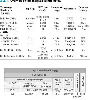
In this paper, we present a comparison of the expected life-time for IoT devices operating in the wireless networks listed in Table 1: beacon-enabled IEEE 802.15.4, the Time Slotted Channel Hopping (TSCH) variant of IEEE 802.15.4e [8], Bluetooth Low Energy (BLE), IEEE 802.11 PSM, and future IEEE 802.11ah. We also consider the emerging long-range technologies (LoRa and SIGFOX) to see how they perform compared to other protocols. We assume IPv6/6LoWPAN protocols whenever possible (see Fig. 1) and carefully
VOLUME 5, 2017
2169-3536 2017 IEEE. Translations and content mining are permitted for academic research only.
TABLE 1. Overview of the analyzed technologies.
FIGURE 1. Protocol stack of the considered technologies.
analyze the energy consumption patterns for duty-cycled MAC layers to derive the lifetimes.
A. MOTIVATION AND RESEARCH GOALS
The motivation for this paper comes from the observation that many different wireless technologies can be used for IoT and there is no exhaustive comparison in the literature of their energy consumption that would help to make right decision about deployment of a given network. Although some char-acteristics of the considered technologies, such as the range or the used bandwidth, are not directly comparable, there is a need for a thorough comparison of the energy efficiency to identify their key factors and limitations. Many overviews of different wireless networks exist [9]–[13], but to the best of our knowledge, no previous work compares a large set of wireless networks for IoT from the energy efficiency point of view while setting them on an equal basis. Some papers just study two technologies [14], [15], but a comparison with other possible solutions is still missing. Such a comparison with all technologies laid on the same basis can bring to light the respective advantages and drawbacks to drive the future developments for improving performance and energy consumption.
Another motivation of our work is to extend the energy consumption models that reflect the operation of duty-cycled MAC layers, which is often neglected in energy consumption studies. Before recent papers that set the principles of the energy model we use [16]–[18], energy consumption models only took into account the following main aspects: transmis-sion power, distance between two nodes, packet size, and path loss [19]–[23]. This approach only modeled the behavior of the physical layer and it did not reflect the operation of
duty-cycled IoT devices in a realistic way. Our goal was to extend the recent realistic energy consumption models to all considered technologies and make them available through an open source tool allowing anybody to play with the network parameters and quickly estimate lifetimes.
Finally, we want to evaluate the impact of pushing the IP protocols to constrained IoT devices by taking into account not only the hardware performance and duty-cycled MAC operation, but also the protocol overhead (headers and frag-mentation), along with the cost of keeping an active connec-tion and time synchronizaconnec-tion between two nodes. In this way, we can evaluate the impact of all layers on energy consump-tion and performance. The overall goal of this paper is to help all users of IoT technologies to choose the technology that best fits their needs from the perspective of energy efficiency. B. ASSUMPTIONS, RESEARCH METHOD,
AND CONTRIBUTION
We consider the case of an energy constrained node (battery-operated or energy harvesting) that generates and uploads data to a sink (uplink traffic). We adopt the view of an IoT device that connects to the network and wants to stay alive for the longest time. We limit the scope of the paper to a single link case, because it is the current most common con-figuration setup, a kind of a baseline for comparisons (note that many papers limit the scope to a single link case, e.g. the analytical energy consumption model of B-MAC proposed by Polastre et al. [24]). Moreover, the topology of all the considered networks except 802.15.4 is a star one in which a node connects to or associates with a main-powered node to obtain Internet connectivity. In the future work, we plan to extend the analysis to multi-hop 802.15.4 and upcoming mesh BLE networks.
Our research method consists of analyzing energy consumption of each technology by considering a real-istic energy model in which the main energy con-sumers (radio transceiver, microcontroller) alternate between active and inactive states (Tx, Rx, Idle, Sleep) with known power consumption patterns and timing con-straints defined by the MAC layers. We derive the model from the previous proposals for 802.15.4/e [16]–[18], extend them to other MAC technologies, and use it to analyze the technologies in function of different parameters.
For the presented analysis, we assume the application traffic workload composed of variable UDP (User Datagram Protocol) packet sizes over IPv6/6LoWPAN protocols when-ever possible (see Fig. 1) or over a given MAC layer oth-erwise. The analysis takes into account the energy spent in data frame retransmissions due to corrupted frames and collisions. We consider the energy consumption for different hardware platform parameters (i.e. energy consumption per state) to find the parameters resulting in the minimal energy consumption. We then adopt the minimal energy hardware platforms to compute the lifetime of the considered technolo-gies for application traffic with varying intensity, Packet Error Rate (PER), and clock precision. The premise is that even if
such an idealized device does not yet exist, it represents the best-in-class energy performance enabling the comparison with other technologies.
The main new scientific contributions of the paper with respect to the state of the art are the following:
• we extend a realistic energy model that takes into account the behavior of the PHY and MAC layers to all considered technologies,
• we develop an open-source lifetime analyzer, a tool for estimating the lifetime of a given network based on the main hardware and MAC parameters,
• we use the analyzer to study the impact of higher layer protocols (fragmentation, protocol overhead), time syn-chronization, and packet losses on the lifetime (main conclusions are summarized below),
• we reveal several new results: i) the power consumed in the Sleep state becomes a determining factor of the device lifetime for low traffic intensities, ii) 802.15.4 consumes less energy than 802.11 PSM for low intensity traffic, which restrains the findings by Tozlu [2], and iii) asynchronous technologies such as LoRa and SIG-FOX achieve long lifetimes when we assume realistic clocks with drift.
• we discuss the suitability of the technologies for repre-sentative applications corresponding to chosen use cases and study the feasibility of energy harvesting solutions. Section VI provides the main conclusions of the comparison.
C. LIMITS OF THE STUDY
The comparison considers networks with different ranges varying from several meters (BLE) to several kilometers (LoRa, SIGFOX). Moreover, they offer different transmis-sion robustness depending on the Modulation and Coding Scheme (MCS) inherent to each technology and chosen trans-mission power. We are aware that energy consumption is only one aspect to take into account when choosing the right technology for a given application use case. Other parameters such as throughput, delay, reliability, coverage range, radiated power, and cost can also be considered.
For instance, it does not make sense to propose the use of short-range BLE instead of long-range SIGFOX when an application requires large coverage. Similarly, there is always a trade-off between the transmission power, the range, and the resulting bit error rate. However, to select the best technology given application requirements (performance, energy sumption) in a specific communication context (ranges, con-ditions), it is necessary to understand the energy limitations of each technology and identify the factors that influence the node lifetime for a given performance level. We provide some information on these aspects in Table 1.
Our analysis also makes some simplifications that influ-ence the precision of the energy consumption predictions: a simple probabilistic model of packet loss, constant bit rate type of the application workload, and single link topology setup.
The four-state energy consumption model is not suffi-ciently precise for some technologies, so we have added a 6-state model for 802.15.4e TSCH in Section V to represent the behavior of this technology better. Since some hardware platforms do not operate according to the 6-state model, we cannot use it for all technologies. Nevertheless, we include the results of both models for TSCH in Section V. More research is further needed to take advantage of switching the microcontroller off during radio activity without spending to much energy in the wake-up phase.
The hardware model assumes instantaneous transitions between states, but in reality, they take some time, which results in additional energy consumption. Finally, we use a linear battery current draw model, but the real battery discharge process is much more complex. Nevertheless, the linear model is not that far from complex recursive models (less than 10%) [25] and we compensate this difference by taking into account parameterable current leakage.
D. STRENGTHS OF THE STUDY
The analyzer presented in this paper gives us a means for quick evaluation of the energy consumption in the main IoT wireless networks. It realistically models the behavior of principal protocol layers and takes into account several factors important for evaluating energy consumption: proto-col overhead including fragmentation, power drained in the sleep state, packet losses, time synchronization, and varying application traffic.
Our objective of developing an analytical tool obviously leads to some simplifications, however, the comparisons with other studies show sufficient accuracy of its results. Considering all energy consumption factors would require a full-fledged simulator.
E. ORGANIZATION OF THE PAPER
To provide an in-depth understanding of energy consumption and keep the paper self-contained, we start with a com-prehensive description of MAC operation for each consid-ered technology in Section II. We then present the proposed energy consumption model and its validation in Section III. Section IV evaluates the impact of hardware parameters on the lifetime and provides the choice of the parameters for the comparisons. Section V presents the results of our analyzer for different application scenarios and identifies the main factors that influence energy consumption. Finally, Section VI concludes the paper.
II. BACKGROUND ON WIRELESS NETWORKS FOR IOT
While this section presents each of the IoT technologies in detail, we need to discuss several specific assumptions adopted in our analysis. First, we assume that the radio and the microcontroller are the most energy-consuming parts of each device. Moreover, we consider the model of energy consumption in which the total energy consumption is com-puted as the power required for each state over the time spent in the state. Our model assumes four different states for an
TABLE 2. Hardware consumption states.
IoT platform: Rx, Tx, Idle, and Sleep illustrated in Table 2 with the modes of each component (we give the details of the power drawn in each state later on).
In addition, we consider a minimal packet structure for analysis, i.e. we do not consider the security overhead within
data, beacon, and ack frames.
We summarize the analyzed IoT standards and technolo-gies below and present their energy consumption patterns as a function of the MAC operation (state, duration).
A. BEACON-ENABLED 802.15.4
802.15.4 [1] is the most popular standard for low-power wireless networks, largely used in industrial applications and subject to continuous development [18], [26], [27]. Its typical targets are low-power embedded communication systems that require a low data rate and low latency.
The 802.15.4 PHY layer uses the 2.4 GHz and sub-1 GHz bands. In the 2.4 GHz band, 802.15.4 splits the spectrum in sixteen 5 MHz-wide channels with a 5 MHz inter-channel space. 802.15.4 supports robust transmissions with DSSS (Direct-Sequence Spread Spectrum) and the O-QPSK (Offset Quadrature Phase Shift Keying) modulation scheme giving a bit rate of 250 kb/s. Multi-hop topologies can extend its relatively short ranges (see Table 1).
FIGURE 2. Data frame structure of 802.15.4 (size in bits).
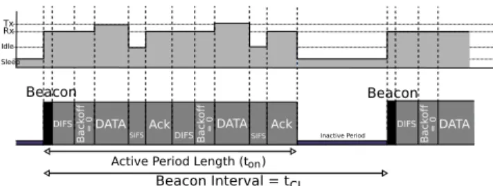
FIGURE 3. Operation of beacon-enabled 802.15.4.
Even if we consider a single link between a leaf node and a sink, the beacon-enabled mode is interesting in multi-hop topologies for saving energy at intermediate and leaf nodes. In this mode, a coordinator node periodically sends a beacon to delimit its superframes and invites neighboring associated nodes to send their data frames (see Fig. 2) during the Contention Access Period (see Fig. 3). Nodes operating
according to the beacon-enabled mode can achieve a low energy consumption because a node can safely turn its radio off during the rest of the superframe and wake up at the next beacon. Periodic beacons allow keeping time synchronization between nodes.
Nodes in beacon-enabled mode use a slotted Carrier Sense Multiple Access with Collision Avoidance (CSMA/CA) access scheme. In our analysis, we neglect the backoff mech-anism to simplify the model. In this mode, transmissions follow the superframe organization shown in Fig. 3 that presents: i) a timeline of a node transmitting data to its coordinator (two acknowledged data frames), ii) the node state corresponding to different phases of the superframe. The superframe duration (SD) is defined as follows [1]: SD = 15360 ∗ 2SuperframeOrder(SO)µs, with SO
max =14. Hence,
the maximum beacon interval is:
Beacon Intervalmax =251.658240 s.
B. 802.15.4e/TSCH MODE
TSCH is part of the 802.15.4-2012 amendment [8] that addresses the need for deterministic access in industrial appli-cations: channel hopping helps the network to mitigate mul-tipath fading and a periodic schedule using dedicated slots, defined by a channel and timeslot, avoids contention. TSCH mainly aims industrial networks that require an increased level of robustness, reliability, availability, and security.
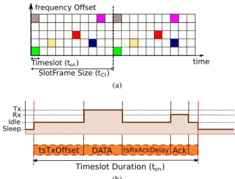
FIGURE 4. TSCH principles. (a) Example TSCH schedule. (b) Operation states in a TSCH timeslot.
Fig. 4a shows an example of a TSCH schedule represented by a slotframe that defines a couple (slot, channel) allocated to a pair of nodes. The standard does not define how to build a schedule and some proposals for scheduling have already appeared [28]–[30]. The TSCH data frame is the same as the classical 802.15.4 one (see Fig. 2), except that the Sequence
Numberfield is omitted.
Once a node has joined the network, there is no need of beacon frames to keep nodes synchronized (except for
Whenever the transmitter wants to send a packet, it turns its radio on at constant tsTxOffset after the beginning of a timeslot (see Fig. 4b). On frame reception, the receiver computes the difference between the frame arrival time and the expected tsTxOffset to adjust its clock with respect to the transmitter. In addition, an acknowledgment frame (ACK) may also contain a timestamp to adjust the clock. However, if there is no data traffic, nodes need to use specific keep-alive messages for synchronization. The maximum interval between keep-alive messages (empty data frame) is set so that the clock drift never exceeds the guard time defined as:
guard time = tsTxOffset − tsRxOffset. (1)
Since we assume a symmetrical clock drift at the receiver and the transmitter:
keep_aliveperiod ≤
guard time
2 ∗ clockAccuracy (2) Given a clockAccuracy of 40ppm and the default values of the standard [8] (Table 52e), we used guard time = 1 ms, which leads to keep_aliveperiod ≈ 12.5 s.
C. BLUETOOTH LOW ENERGY (BLE)
BLE is the low-energy version of the Bluetooth standard [4]. BLE is mostly used for monitoring applications, such as heart rate monitors or remotely controlling the temperature of a room. An important advantage of the BLE technology is its popularity—BLE is already deployed in the majority of smartphones and it is largely used for mobile applications. It defines a master/slave relationship between two nodes in a star topology. BLE does not yet support the mesh topology, but a scatternet topology is already available in version 5.0 (a collection of trees) since a node can be a slave and a master at the same time in different connections. The 6lo IETF working group defines the adaptation layer to transmit IPv6 packets over BLE [31].
BLE nodes split the 2.4 GHz ISM frequency band into 37 dedicated channels, plus 3 advertising channels. The width of all channels is 2 MHz with inter-channel spacing of 2 MHz. BLE uses the GFSK (Gaussian Frequency-Shift Keying) modulation to obtain a maximal 2 Mb/s bit rate and takes advantage of frequency hopping spread spectrum for robust transmissions. The recent version 5.0 allows fitting different ranges and robustness requirements with four coding schemes leading to several PHY rates: 125 kb/s, 500 kb/s, 1 Mb/s, and 2 Mb/s. In this analysis, we focus on the highest available data rate that results in a minimal energy consumption for similar overhead. BLE nodes can change frequency either periodically or at some logical time depending on the fre-quency hopping mode.
BLE offers two different communication modes:
asyn-chronous transmissions that involve advertisement
pack-ets (ADV) and synchronous transmissions in connected mode. Asynchronous transmissions only support sending a small number of bytes, so we focus on the connected mode in which slave nodes discover and connect to a master. In this
FIGURE 5. BLE data frame structure (size in bits, if not explicited).
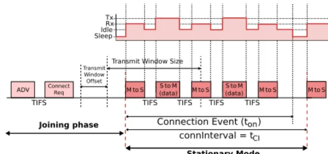
FIGURE 6. BLE operation.
mode, a joining node sends ADV frames on one or several of the three advertising channels scanned by a master node. After its discovery by the master node, the slave node wakes up at the beginning of each connInterval and waits for a unicast-poll frame from its master before sending its data packet (see Fig. 5) as shown in Fig. 6.
The slave and the master achieve time synchronization through polling packets sent with a maximal period of 8.0 s by the master. If there is no data traffic during a long period, the slave needs to wake up at least every 4 connIntervals, which corresponds to a period of 32 s, to listen to a poll packet from its master and reply with an ACK.
FIGURE 7. 802.11b PSM data frame structure (size in bits).
D. 802.11 PSM
802.11 PSM is an energy-optimized mode specified in the 802.11b version. It targets energy efficiency by enabling active/sleep duty cycles for associated nodes. In 802.11b, nodes can transmit on one of the thirteen 22 MHz wide channels separated by 5 MHz. The 802.11b revision speci-fies Complementary Code Keying (CCK) of 8 bits/symbols, which results in a bit rate of 11 Mb/s. 802.11 PSM supports a star topology with the Basic Service Set (BSS) and an Access Point (AP). Fig. 7 shows the data frame structure.
Fig. 8 presents the principles of the Distributed Coordi-nation Function (DCF) used in 802.11b PSM when a node sends two data frames in a row to an always-on Access Point.
FIGURE 8. Operation in 802.11 PSM mode.
DCF requires nodes to stay in Rx mode for a random period of time before sending data, competing with other nodes to access the channel. In our setup however, there is no con-tention. The usual value of the beacon interval is 100 ms in classical 802.11 networks. However, the listen interval field of the beacon encodes the number of time units on 2 B, which leads to a maximal value of ∼ 18.6 hours.
E. 802.11ah or Wi-Fi HaLoW
The last version of 802.11ah draft standard [5] specifi-cally addresses main IoT requirements: an increased range, increased reliability, and low energy consumption. It can be seen as an optimized 802.11ac PHY layer [32] on sub-1 GHz frequency bands in the PSM mode. The choice of the sub-1 GHz band comes from the objective of limiting interference in the crowded 2.4 GHz band. Moreover, the European limi-tation of the duty cycle in this sub-band is not applicable for 802.11ah since the transmission scheme is based on Listen
Before Talkand Adaptive Frequency Agility. As in 802.11ac, there are 10 available MCS operating in bands of different widths. We consider two extremes: MCS giving the minimum and maximum data rates. The minimum data rate is given with MCS10 and 1 MHz band (denoted as 10_1), using a BPSK modulation, with a 2*code repetition. The maximum data rates are given by MCS8 in Europe, 2 MHz band (8_2) and MCS9 in the US, 16 MHz band (9_16), using a 256-QAM modulation.
FIGURE 9. 802.11ah data frame structure (size in bits).
802.11ah uses DCF as in 802.11 PSM (see Fig. 8). The
Restricted Access Window(RAW) access scheme is also
pos-sible [33], but as DCF and RAW obtain similar performance in a small network [34], we only consider DCF. Fig. 9 shows the structure of a data frame.
F. SIGFOX
SIGFOX is an ultra-narrow-band technology that operates in the 868 MHz frequency band in Europe and 915 MHz in the US. The available PHY rates are 100 b/s for a 100 Hz bandwidth and 1000 b/s for a 1 kHz channel width in Europe (and 600 b/s in the US). With sensitivity of −140 dBm, its
announced range is around 40 km. SIGFOX devices can transmit up to 140 messages per day to the base station with a maximum user payload of 12 B, so we assume that applications encapsulate their data directly in MAC frames. Moreover, European Telecommunications Standards Institute (ETSI) regulation imposes a capacity limitation: SIGFOX operates in the sub-1 GHz band, which leads to a maximum duty-cycle of 0.1% or 1% in 863 − 870 MHz (depending on the selected sub-band). Note that 140 messages per day corresponds to the limitation of 1% duty-cycle with a 100 b/s SIGFOX implementation.
FIGURE 10. SIGFOX Uplink packet structure (size in bits).
At the MAC layer, a device that wants to transmit data, encapsulates it within a packet (see Fig. 10) and trans-mits three times on different random frequencies with dif-ferent channel encoding at each transmission. The network can send a downlink packet of 8 B, but we do not take into account downlink transmissions in our analysis. While SIGFOX available data rates are low, the long range of the technology and ease of deployment are important key features for many IoT applications.
SIGFOX is an asynchronous technology (as is LoRa)— nodes do not need to wake up at a specific instance for synchronization. Hence, the energy consumption model of SIGFOX is simpler than for other technologies: nodes are in Tx state while transmitting data and in Sleep state between transmissions. Note that SIGFOX defines an inter-transmission time during which the node is in Idle mode. As this time is negligible compared to the duration of the data frame, we do not take it into account.
G. LoRa
For long-range IoT applications, the LoRa Alliance proposes a cellular topology with base stations/gateways that receive packets from devices and relay the data to a server on a TCP connection. Actility (a LoRa partner) and other partners enabled 6LoWPAN on top of LoRa, but for a fair comparison with SIGFOX, we have assumed the transmission of applica-tion data directly over the MAC layer.
LoRa operates in the same band as SIGFOX and 802.11ah, and uses a proprietary modulation based on the Chirp Spread Spectrum (CSS) that trades data rate for sensitivity within a fixed frequency band. The LoRa modulation offers data rates from 0.25 to 11 kb/s in the European frequency band. 250 b/s corresponds to a spreading factor of 12 for a bandwidth of 125 kHz, whereas 11 kb/s results from a spreading factor of 7 and 250 kHz of bandwidth. Devices can also use FSK mod-ulation to reach a higher data rate of 50 kb/s (not considered in the analysis).
In our analysis, we assume a Class A LoRa device that transmits frames as soon as the data is available (no Listen
Before Talk): LoRa devices need to comply with the ETSI regulations of the 868 ISM band. The energy consumption model of LoRa includes the Idle state between transmissions and ACK, and the Rx state during ACK.
FIGURE 11. LoRa packet structure (size in bits).
Fig. 11 shows the LoRa data packet structure. The maxi-mum user data size depends on the data rate. For the minimal and the maximal data rate in Europe, the maximum data sizes are respectively 59 and 250 B. As the LoRa preamble is composed of eight symbols, a node may spend long time in Rx (resp. Tx) mode depending on the chosen modulation. It is however required to accurately synchronize the nodes to achieve the LoRa coding gain necessary to demodulate the LoRa signal under the noise floor.
III. PRINCIPLES OF ANALYZING ENERGY CONSUMPTION
We present below the fundamentals of our analyzer that computes energy consumption and the lifetime of the con-sidered wireless technologies. Compared to a simulator, an analytical approach presents the advantage of a shorter exe-cution time and a lower development effort while providing sufficient precision. Note that chip manufacturers adopt a similar approach, for instance Linear Technology proposes an analyzer for its products [35]. Our analyzer is developed in Python and available in the public domain.1
A. ENERGY CONSUMPTION MODEL
We use a model derived from the work by Vila-josana et al. [16] to express the energy consumption in interval t as follows:
E(t) =X
S
PS× tS, S ∈ {Tx, Rx, Idle, Sleep} (3)
where PS is the power consumption in state S and tS is the
time spent in state S during t. tS comes from the analysis
of the operation of each wireless technology presented in section II. We assume a star topology with one link between an energy-constrained leaf node for which we want to find the lifetime, and a main-powered sink. The analysis considers upward application traffic (such as periodic reporting) to the sink. To take into account IP connectivity, we consider an adaptation layer (6LoWPAN or 6Lo) if needed, and IPv6 run-ning on top of a given PHY/MAC layer for each technology whenever possible (see Fig. 1). However, because of small packet sizes, the long-range technologies support application data directly on top of the MAC layer.
Moreover, the analysis assumes the stationary state, i.e. the leaf node is already associated with the sink.
1https://gitlab.imag.fr/morine/iot-analyzer
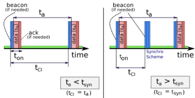
FIGURE 12. Variables used to compute energy consumption and device lifetimes. (a) Without synchronization scheme. (b) With synchronization scheme.
B. APPLICATION MODEL AND LIFETIME COMPUTATION Fig. 12 illustrates the definition of the main variables we use to compute the energy consumption while analyzing the operation of a given MAC protocol achieving the max-imum throughput. If a node has to fragment a packet, it will send fragments in consecutive frames. The synchronization scheme corresponds to the communication for maintaining synchronization between two nodes based for instance on beacon or poll frames.
We define the following variables:
• ta, Application Period is the time interval between two instants of data generation by an application.
• sa, Application Data Size is the size of the data gen-erated by the application each ta. sa is the useful data
at the application layer. We then add the overhead of each protocol and take into account fragmentation if necessary.
• ra, Application Throughput corresponds to the generated
application data rate in bits/s (b/s): ra=sta a.
• tsyn, Maximal Synchronization Period corresponds to the
interval after which a node needs to wake up for time synchronization. The period is required to keep an active association between devices. If there is no communica-tion during an interval longer than tsyn, nodes lose their
association with the network and will need to rejoin, potentially at the cost of greater energy consumption. • tCI, Check Interval is the time between two wake-ups
of a node defined by tCI = min(ta, tsyn). A data
trans-mission may serve for synchronization, but if there is no application data to send, nodes need to communicate each tsyn(see right part of Fig. 12).
• ton, Active Period is the maximum time a node stays
awake, i.e. when it is in a state different from Sleep during tCI (see Figs. 3, 6, 8, and 4b).
• Lt, Lifetime of a node corresponding to the time a node
can run on some initial energy E0.
To estimate device lifetimes for each protocol, we select the MAC parameters of each protocol to support ra, the
applica-tion throughput with the minimal energy consumpapplica-tion, so we set ton to the minimal duration to transmit sabytes of data.
For example, we choose the 802.15.4 SD parameter to reach the optimal tonperiod, given the value of saper tainterval.
If a technology cannot support given application through-put ra, it does not appear on the curves. The representation of
a technology stops when the application traffic corresponds to the maximal capacity of the given protocol.
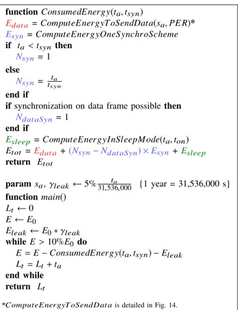
FIGURE 13. Lifetime computation algorithm.
Based on the variables and the operation principles of each MAC layer (explained in Section III-A), we compute the energy consumption over one ta with Eq. 3, in which PS,
the power consumption in state S, is multiplied by tS, the
time spent in state S during one ta. Our lifetime algorithm
(see Fig. 13) computes the energy consumed per ta as a
function of application throughput ra and derives Lt, the
lifetime of a node. Ltis the number of taa node can run until
the initial energy E0is exhausted. C. PACKET LOSS MODEL
For technologies that use retransmissions, we take into account lost data packets due to imperfect transmission con-ditions or collisions in the following way. Let pfer and prer
be the packet error rate in the forward, respectively reverse, direction: a data packet sent from a node will be lost with probability pferwhile its acknowledgment will suffer from the
loss probability of pr
er. The probability of a lost transmission
at the MAC layer is thus:
PER = pfer +(1 − pfer) × prer. (4)
If prer is small compared to pfer (small ACK packets), the
probability reduces to PER = pfer. Assuming packet loss
probability PER, a node performs the following number of transmissions on the average:
Ntr =
1
1 − PER. (5)
In the comparisons, we will choose a given level of PER and compute the energy consumption required to send Ntr data
frames followed by an ACK for one packet generated by the application layer.
FIGURE 14. Algorithm of the ComputeEnergyToSendData function.
Fig. 14 gives the details of the ComputeEnergyToSendData function in which we take into account the energy con-sumption due to data retransmissions within each application period ta.
D. BATTERY MODEL
We assume an initial battery energy of E0 = 13.5 kJ corre-sponding to two AAA batteries (1250 mAh under 1.5 V each) and a simple battery model with leakage Eleakof 5% per year,
as well as a cutoff voltage when the residual energy reaches 10% of E0. For fair comparisons, we assume the same battery for all technologies even though a smaller battery can be used for some protocols.
IV. IMPACT OF HARDWARE PLATFORMS AND CHOICE OF THEIR PARAMETERS
To compare the technologies on the same fair basis, we need to choose the hardware parameters for the power consump-tion values. The idea is to identify the parameters that result in the smallest energy consumption for each technology. A. TECHNOLOGY-DEPENDENT PARAMETERS
We start with the main parameters of the standards, presented in Table 3. We also assume 802.15.4 CCADuration of 128µs and use the default TSCH interval values (see TSCH-MAC PIB attributes [8]):
• timeslotLength =10 ms,
• tsTxOffset =2.120 ms, • and tsRxAckDelay = 800µs.
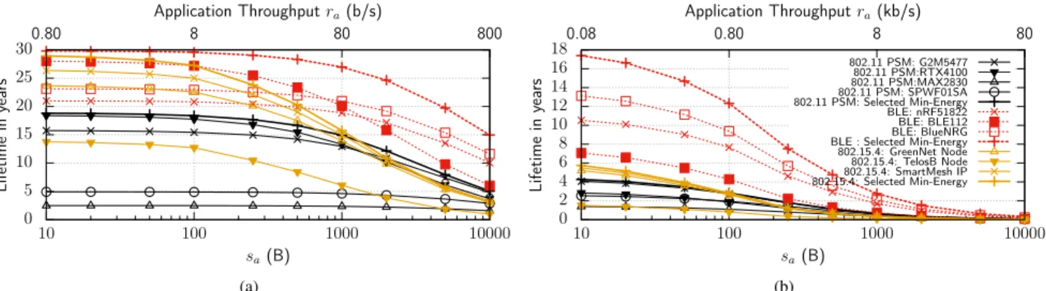
FIGURE 15. Impact of hardware platforms on the lifetime, E0=13.5 kJ. (a) Varying sa, constant ta=100 s. (b) Varying sa, constant ta=1 s. The legend applies to both (a) and (b).
TABLE 3. Technology parameters.
TABLE 4. Hardware platform parameters.
B. HARDWARE PLATFORM PARAMETERS
We consider several hardware platforms summarized in Table 4 and evaluate the impact of their power consumption parameters of Table 2 on the lifetime. By a hardware platform we mean a SoC with a microcontroller and a radio module.
Fig. 15 compares the lifetimes for the initial energy
E0 =13.5 kJ, constant ta, and varying safrom 1 B to 10 kB.
This figure clearly shows an important impact of the hardware parameters: for instance, the lifetime of 802.11 PSM varies from ∼ 1.5 to ∼ 4 years for different 802.11 PSM platforms, when ta = 1 s (see Fig. 15b) and ra = 10 B/s. The effect
is even more important for ta = 100 s (see Fig. 15a).
Large differences for 802.15.4 and BLE platforms are also notable.
2assuming GreenNet STM32 CPU.
We can notice that the lifetimes are not ranked by the values of PTx and PRx, e.g. most of the 802.11 PSM
plat-forms perform better than 802.15.4 TelosB even though the TelosB Tx and Rx power consumption is lower than that of 802.11 PSM. Actually, the power consumption in these states is a decisive factor for high data rates (small ta), but when the
data rate is lower (e.g. ta = 100 s), the Tx and Rx power
consumption becomes less important. In this case, contrary to the common belief, the technologies are ranked by their
Psleeppower, since nodes spend much more time in the sleep
state. Hence, hardware designers should also concentrate on this value in addition to minimizing the Tx and Rx power consumption.
TABLE 5.Hardware parameters used for comparisons.
For a fair comparison, we have examined a range of hard-ware platform solutions and used the best-in-class param-eter value for each technology (denoted by the Selected
Min-energyin Tables 4, 5, and Fig. 15). In doing so, we have effectively modeled a composite platform that offers ideal-ized performance and results in the best trade-off between their Pidle, PTx, and PRx parameters. Here our assumption
is that while such an idealized device may not yet be on the market, it is feasible that a single platform offering such best-in-class performance exists. Tables 5 and 6 summarize the chosen hardware parameters that we use to generate the remaining results of the paper.
Moreover, we have chosen to use the same parameters for BLE, 802.15.4, and TSCH because their hardware design is similar (same transmission power and modulation
com-plexity). Hence, we adopt the lowest value of GreenNet for PIdle, the SmartMeshIP values of PRx and PIdle, along
with the lowest Psleep value of BLE112. Choosing a
com-mon platform presents the advantage of a fair comparison of the protocols instead of comparing hardware platforms. However, we cannot extend this approach to every technology—we keep a large difference in Rx and Tx power consumption between the 802.11 standard and the other technologies. The difference in the output power (0 dBm compared to 14 and 18 dBm) is necessary to reach 802.11 ranges and therefore justifies a higher Tx power consump-tion. Different modulation schemes explain the difference in the Rx power consumption—demodulating a more complex scheme costs more energy to achieve an acceptable Bit Error Rate (BER).
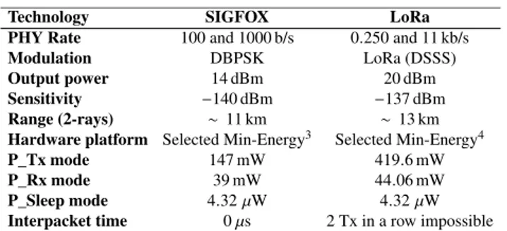
TABLE 6. SIGFOX and LoRa parameters.
For long-range technologies, we adopt the parameters in Table 6.
C. VALIDATION OF THE ANALYZER
To validate our analyzer, we have compared its results with the SmartMeshIP power estimator [35] of TSCH provided by Linear Technology, using the lowest power mode. We have configured a star topology with one node sending 10 bytes to its parent at each application period ta=100 s (called
report-ing interval) with 100% path stability. The estimator assumes a keep-alive period of tsyn∼ 4.083 s (∼ 25 keep-alive frames
during 100 s), but it does not exploit the possibility of time synchronization during data exchange. In this setup, the total average mote current estimated for a downlink slotframe of 1024 slots is 4.3 µA for a voltage of 3.6 V. In a comparable setup, our analyzer gives the average current consumption of 4.317 µA, less than 1% error.
We have also compared the average energy consumption of 802.15.4 with the measured value on the GreenNet plat-form [18]: the average current consumption was 3µA for
BO = 4 (Beacon Interval of 240ms) with the possibility to skip beacons by the leaf node with a maximum time of tsyn,
SO =1 (Superframe Duration of 15.36 ms), and application 3Based on TD1202 [46] with GreenNet microcontroller and BLE112
power in sleep state.
4Based on SX1272 [47] with GreenNet microcontroller and BLE112
power in sleep state.
period ta=4 min. In an equivalent setup, our analyzer
com-putes an average current consumption of 2.46 µA. The 18% difference is mainly due to a simplification inherent in our model that does not take into account the energy consumption of state transitions, nor that of the temperature sensor used in the GreenNet measurements.
In addition, we have compared the 100 B data frame perfor-mance for BLE and 802.15.4 with the perforperfor-mance reported by Siekkinen et al. [15]. We modify BLE parameters to fit BLE4.0 specification [48], to compare equivalent scenarios. Our results for BLE gives 460 KB/J, while 433 KB/J was reported by Siekkinen et al. Similarly, we find 180 KB/J for the 802.15.4 standard, while Siekkinen et al. reported 168 KB/J. In both cases, the difference is less than 7%.
To validate the analyzer for long range technologies, we have compared its output with the values measured by Martinez et. al [17] for transmission of a single 12-byte data packet (i.e. the maximum size for the SIGFOX technol-ogy). In the previous section, we have assumed data packets without security for all technologies, but to set up a fair comparison, we have added an additional overhead of 2 B to the minimal SIFGOX packet presented in Fig. 10, because SIGFOX imposes the use of HMACs for message authentica-tion at the MAC layer. Martinez et al. measured a current load of 50 mA for three consecutive transmissions of ∼2 s each. Assuming a 3 V voltage, this value corresponds to 900 mJ. Our analyzer computes a transmission time of 6.24 s with an energy consumption of 917.28 mJ (less than a 5% difference). Finally, we have compared our results with LoRa measure-ments [17]: for transmission of a 15 B data packet and assum-ing a maximum LoRa spread factor, the measured energy consumption is ∼213 mJ. In a similar setup, we compute a consumed energy of 224 mJ, which corresponds to a differ-ence of ∼5%.
These comparisons show that our analyzer yields data within 5%-7% of most published measured values and broadly confirms the consistency of our approach.
V. COMPARISONS OF DEVICE LIFETIMES
Having confirmed the validity of our analyzer, we now present the predicted device lifetimes for the following three cases:
1) assess the impact of application parameters without any packet loss or clock drift.
2) evaluate the impact of a limited packet loss probability without clock drift.
3) assess the impact of imperfect clocks with clock drift (but no packet loss).
A. IMPACT OF APPLICATION PARAMETERS, NO PACKET LOSS
Fig. 16 presents the comparison of the lifetime for fixed values of application period ta = 1 day, 100 s, 1 s, and
10 ms, and for varying data size sa, which results in varying
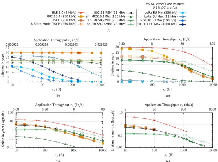
FIGURE 16. Different taand data size sain bytes, leading to varying ra, impact lifetime for a starting energy E0=13.5 kJ, PER = 0. The bottom x-axis is
the data size in bytes per tawhile the top x-axis presents the corresponding data rate rain b/s. No packet loss or clock drift is assumed. (a) legend. (b) varying sa, constant ta=1 day. (c) varying sa, constant ta=100 s. (d) varying sa, constant ta=1 s. (e) varying sa, constant ta=10 ms.
With the separation of application period taand data size
sa, we can distinguish between the energy consumption of
an application that generates sa =10 B every second and an
application sending sa = 600 B every minute, even though
for both cases ra=80 b/s. In the first case, there are 60
trans-missions with the corresponding protocol overhead, whereas in the second case, the application only sends the minimum number of frames, depending on the chosen technology maxi-mum data packet size. This effect explains, for instance, why the lifetime for a given ra(e.g. 80 b/s) is higher in Fig. 16c
than in Fig. 16d.
The figures include the results for TSCH (marked as 6-State Model TSCH with dashed lines) based on a more sophisticated model of energy consumption with two addi-tional states available on recent 802.15.4 platforms that can turn their microcontroller off when transmitting [16] (see Fig. 17).
For the sub-1GHz frequency band, the ETSI regula-tion recommends a certain duty cycle depending on the used sub-band (e.g. 0.1% for 863-870 MHz and 1% for
FIGURE 17. 6-State energy consumption model of TSCH.
868-868.6 MHz) when no Listen Before Talk and Frequency
Agilitymechanisms are used. Hence, in our study, we
dis-play the result for 0.1% as a solid line and the result for 1% as a dotted line for the concerned technologies (SIGFOX and LoRA). The duty cycle limit of 1% determines the maximal capacity of SIGFOX at 1 kb/s and 100 b/s. More-over, the marketing limitation of SIGFOX to 140 packets per day further limits the capacity of SIGFOX at 1 kb/s and it corresponds to the 1% duty cycle at 100 b/s.
1) VERY LOW TRAFFIC INTENSITY (ta=1 DAY)
Fig. 16b shows the lifetime comparison for very low traffic intensity ta = 1 day corresponding to the operating
condi-tions of long-range technologies. We observe that BLE and 802.15.4 achieve the best lifetimes. LoRa performs remark-ably well with an only slightly lower lifetime compared to the short-range BLE and 802.15.4 standards. SIGFOX achieves similar lifetimes to LoRa only for extremely low ra, since the
available bit rate of SIGFOX is 11 times smaller than that of LoRa.
SIGFOX and LoRa consume more energy as the data size saincreases. Their lifetime drops because they can only
handle small data packet sizes—fragmentation often occurs, which increases the overhead, and consequently the energy consumption. Moreover, to reach the targeted long ranges, they use high transmission power, which contributes to the increased energy consumption when they need to transmit for longer periods.
As seen in Fig. 16b and 16c, SIGFOX and LoRa suffer from capacity limitations due to the ETSI regulation in the sub-1GHz band. In addition, ETSI regulation requires that nodes do not transmit more than a certain number of consecutive frames per hour. Thus, SIGFOX or LoRa nodes that must transmit for more than 3.6 s (for 0.1% duty cycle) will have to delay some packets to the next hour, which impacts latency.
A SIGFOX node requires three transmissions to send one data frame, before it is acknowledged by the base station. In this case, the limit of messages per hour leads to an incapacity to respect the duty cycle limitation in the 863 − 870 MHz with the rate of 100 b/s. Hence, we advise at least the use of the 1% tolerable sub-band to compete with other IoT technologies.
802.11ah performs significantly worse than LoRa for small data sizes and outperforms it for larger data sizes. 802.11ah also outperforms 802.11 PSM and obtains similar perfor-mance to TSCH. Note that all 802.11ah curves are overlaid in Fig. 16b: we have used the same Psleepvalue for the three
802.11ah technologies (see Table 5). As Psleep value is the
determining factor for a synchronized technology for very low data rates, we understand the overlay of the curves.
2) LOW TRAFFIC INTENSITY (ta=100 s)
For sporadic application traffic, BLE achieves the longest lifetime with the 802.15.4 performance not too far behind for small data sizes (see Fig. 16c). For larger data sizes in Fig. 16c, the US variant of 802.11ah with 16 MHz of band-width becomes an interesting solution after BLE. In these conditions, the important overhead of 802.11ah packets is mitigated by a larger maximum data size. For this reason, the fragmentation happens less often than for BLE, which decreases the ratio overhead/data for 802.11ah.
Contrary to the findings by Tozlu regarding 802.15.4 and 802.11 PSM [2], [49], Fig. 16c shows that 802.15.4 consumes less energy in most cases of low data traffic (up to throughput of 80 b/s) and obtains much longer lifetimes. We can explain
this result with the lower energy consumption of our 802.15.4 platform compared to TelosB used in the paper by Tozlu—as explained earlier, we have chosen the most efficient platform to compute the lifetime of 802.15.4 (see Table 4). The lifetime of 802.11 PSM becomes better than 802.15.4 only for very long packets (greater than 1.5 kB), not a usual size for IoT applications.
3) MEDIUM AND HIGH TRAFFIC INTENSITY (ta=1 s, 10 ms) For medium and high intensity traffic (see Fig. 16d and 16e, note also the logarithmic y-axis), BLE obtains the longest lifetime although 802.15.4 is traditionally expected to be better.
We can identify mainly two reasons for this result: • The 802.15.4 PHY layer is less efficient than BLE due
to a spreading factor of 8 that reduces the bit rate of 802.15.4 from 2 Mb/s to 250 kb/s, whereas BLE uses the maximum rate of 2 Mb/s. Hence, the bit rate of BLE is 8 times higher than 802.15.4, which leads to a lower energy consumption.
• Fragmentation in 802.15.4 starts from 120 B of useful information, whereas BLE starts fragmenting at 245 B. Since the overhead for a data frame does not depend on the packet size, 802.15.4 is less efficient than BLE for packets bigger than 120 B.
To validate this explanation, we have changed the bit rate of 802.15.4 to 2 Mb/s and set the data frame size to 245 B. In this setup, 802.15.4 comes close to BLE (as shown in Fig. 19).
Moreover, Figure 19 displays the variation in terms of the BLE energy efficiency performance when selecting different modes of Bluetooth Specification 5.0 [4]: the highest avail-able data rate leads to a lower energy consumption because it results in the minimal time in radio consuming modes for similar overhead (see BLE data packets in Fig. 5).
Our results confirm the findings by Siekkinen et al. [15]. They showed that, in the stationary phase, 802.15.4 transmits less data than BLE for the same amount of energy. Siekkinen et al. also obtained their results on a hardware platform equiv-alent to BLE and 802.15.4. BLE is thus the best technology in terms of the energy consumption for medium and high data rates. Nevertheless, it suffers from capacity limitation for larger data sizes. Note that the case presented in Fig. 16e corresponds for some technologies to always-on nodes, when operating at their maximum capacity (represented by the end of a curve).
For sa > 100 B, 802.11 PSM outperforms 802.15.4
(see Fig. 16d) and becomes the second most energy-efficient technology up to sa > 500 B, for which US-only 802.11ah
(MCS9, 16 MHz) with high modulation rates and large band-width becomes the most energy-efficient technology.
We note that the performance of 802.11ah with a smaller channel bandwidth, even with high modulation indices such as the maximum European rate (MCS 8, 2 MHz, 7.8 Mb/s), is worse than or equivalent to that of 802.11 PSM due to the difference in the data rate.
FIGURE 18. Lifetime for varying ra, No clock drift, E0=13.5 kJ, Average Packet Error Rate (PER) = 0.2. (a) legend. (b) varying sa, constant ta=1 day. (c) varying sa, constant ta=100 s. (d) varying sa, constant ta=1 s. (e) varying sa, constant ta=10 ms.
FIGURE 19. Liftime for different BLE 5.0 modes and comparison with theoretical 2Mb/s 802.15.4 (varying sa, constant ta=1 s).
We can also observe that the lifetime of 802.11ah MCS10, 1 MHz, 0.15 Mb/s is consistently worse than the other tech-nologies. To obtain a longer lifetime comparable to BLE or 802.15.4, we will need to lower the default transmission power of this variant of 802.11ah to 0 dBm, which will decrease the range, the key objective of 802.11ah.
B. ROBUSTNESS TO POOR CHANNEL CONDITIONS Fig. 18 presents the impact of the packet loss probability
PER = 0.2 on the lifetime. We have chosen the value
of 20% packet loss to represent a significant impact of chan-nel conditions and interference on transmission quality. It is also usually adopted as a threshold below which a wireless link is considered of low quality and not used for transmis-sions. We can only note a slight variation in the absolute lifetime values: the relative positions of the curves do not change. For instance, the BLE lifetime for ra=800 b/s with
ta =100 s drops from ∼ 15 years to ∼ 13.5 years, but still
stands as the less consuming technology. C. IMPACT OF THE CLOCK DRIFT
To evaluate the impact of handling the clock drift between nodes, we assume that nodes have imperfect clocks C(t) with a given bounded drift1 such that |dCdt(t) −1| ≤ 1. A typical value of1 is 40 ppm for crystal clocks. As both clocks at the transmitter and the receiver may diverge from the perfect clock, the maximum difference between their drifts is bounded by 21. To compensate the clock drift during Check Interval tCI, we need to add a guard interval Tgsuch
that:
TABLE 7. Lifetimes of representative applications, 40 ppm Clock drift, PER = 0.2, and maximum European available rates.
For instance, if tCI = 100 s and1 = 40 ppm, the guard
interval is 8 ms.
FIGURE 20. Timing relationships.
Fig. 20 presents timing relationships between a transmitter and a receiver that need to be awake for a data transmission. The first case assumes perfect clocks so Tx and Rx happen at the same time, which is the baseline case we used to generate Fig. 16. Three other cases illustrate the operation with a guard interval Tgtolerating a maximal relative drift
of 21 (see Eq. 6) and the situation with different values of relative drift (−21, 0, and +21). Note that the case of −21 corresponds, from the energy consumption point of view, to the same situation as the case without the guard interval. Hence, Fig. 16 also gives us the values for −21.
To show the impact of the guard interval and the clock drift on the energy consumption, we have chosen to generate the results of Fig. 16 for the drift of +21 (with 1 = 40 ppm) for which the receiving node needs to stay awake during the longest interval: Fig. 21 shows the corresponding results. We can see that for all synchronous technologies, the time wasted during the guard interval Tgin Rx state leads to
con-siderable shorter lifetimes, more than 20% shorter for ta =
1 day and BLE (approximately 23.5 years compared to 30). Note also that for higher traffic intensity, the influence of these factors is smaller, so Fig. 21c is almost the same as Fig. 16d. In this case, small tamitigates the wasted time of
Tg, since Tgis proportional to tCI that depends on ta.
The impact of the clock drift on the TSCH lifetime is smaller than for other technologies: less than 10% for
ta=1 day with the enhanced state model since TSCH already
specifies a default guard interval of 1 ms to compensate for an imperfect clock.
For ultra low traffic intensity, LoRa and SIGFOX achieve the best lifetimes, the same ones as previously, thanks to their asynchronous operation: they do not need to wake up in advance to compensate for the clock drift.
These results call for an adaptive synchronization scheme. Instead of consuming too much energy in guard time and synchronization maintenance, it may be beneficial for a node to lose association, and then reconnect when needed for a data exchange. For example, to maximize efficiency over the long term, a BLE node would disconnect from the network during sleep mode, then reconnect during wake-up. There is an additional overhead for reconnection, but it may be smaller than the overhead due to clock synchronization. Nevertheless, we note that some mechanisms of clock drift compensation already exist to cope with the drift issue [50].
D. LIFETIMES OF REPRESENTATIVE APPLICATIONS Our study aims at helping engineers and IoT application developers to select the best technology depending on given application requirements. Table 7 summarizes the lifetimes one can expect in a given representative application assuming the optimal operating conditions of an IoT device with two AAA batteries. The analyzer computes the lifetimes for the corresponding application data rates (sa/ta) presented in the
first column of Table 7.
E. ENERGY HARVESTING IoT DEVICES
In this section, we address the issue of IoT devices that harvest energy from the environment and store energy in a small capacity battery (e.g. 20 mAh). Such devices do not have a fixed initial amount of energy that determines their lifetime, but instead, they harvest energy intermittently and then consume it when operating.
TABLE 8.Harvested power.
We take the example of a GreenNet node with a solar panel of '18 cm2 [18] with the indoor and outdoor values of the harvested power presented in Table 8.
FIGURE 21. Lifetime for different ra, Clock drift of +21 = 80 ppm, E0=13.5 kJ, and PER = 0. (a) Legend. (b) ta=1 day, 21 = 80 ppm. (c) ta=1 s, 21 = 80 ppm.
FIGURE 22. Average consumed power per ta, PER = 0.2. (a) Legend.
(b) ta=1 s, 21 = 80 ppm. (c) ta=100 s, 21 = 80 ppm.
Fig. 22 presents the average consumed power per tafor all
technologies. To the right, we mark the level of the intake power for a given light intensity. So, all curves below a given
horizontal harvested power line are theoretically feasible, i.e., a device will have the sufficient power during tato operate.
Our results show that only BLE and 802.15.4 can operate with a typical indoor light intensity of 300 lx. The light inten-sity of 8000 lx is sufficient for all technologies, but devices need to be located 5 cm at most from the light source. Finally, we can see that an outdoor, full-sun scenario can support all technologies, but applications can be vulnerable to variations in the levels of outdoor light.
VI. CONCLUSION AND FUTURE WORK
Our comparison reveals several results not previously brought up in the literature:
1) Assuming ideal clocks, we found that:
• BLE offers the best lifetime for all traffic intensi-ties in its capacity range.
• For ultra low traffic intensity, LoRa performs remarkably well with an only slightly lower lifetime compared to the short-range BLE and 802.15.4 standards. 802.11ah performs signifi-cantly worse than LoRa for small data sizes and outperforms it for larger data sizes.
• For low and medium traffic intensity, the rela-tive ranking is: BLE, 802.15.4, TSCH, and 802.11 technologies with the latter becoming interesting solutions for larger data sizes.
• For high data traffic intensity, 802.11ah with a larger bandwidth and 802.11PSM are the less consuming technologies when BLE reaches its capacity.
2) When we assume a guard time to compensate the clock drift in synchronous technologies, the asynchronous LoRa and SIGFOX technologies obtain the best life-time for low intensity traffic.
3) Contrary to the common belief that power consumption in Sleep state is negligible, Psleep becomes a
deter-mining factor of the device lifetime for low traffic intensities while the consumption in Tx and Rx states still remains important for higher traffic intensity. 4) Taking into account the energy spent in data frame
retransmissions due to corrupted frames and colli-sions does not change the relative ranking of the technologies.
5) The current long-range technologies operating in the sub-1 GHz frequency band with important duty cycle limitations, which reduces their capacity, are not ready to support energy harvesting yet.
We have also shown that 802.15.4 consumes less energy than 802.11 PSM for low intensity traffic, which restrains the findings by Tozlu [2]: the lifetime of 802.11 PSM is only better than 802.15.4 for higher traffic intensity and longer packets.
With respect to the existing literature, our paper provides a unique contribution in several aspects. First, our paper goes beyond several existing comparisons of IoT technolo-gies and PHY/MAC layers for sensor networks [9]–[13] that described the features of different solutions and their limitations without proposing a comparison on an equal basis. Some papers limited their analysis to two technolo-gies: 802.15.4 vs. 802.11ah [14] and BLE vs. 802.15.4 [15] by using different energy consumption metrics: energy to transmit a packet (mJ/packet) vs. energy utility (kB/J), which makes transitive comparisons difficult.
Second, with respect to energy consumption models, much research focused on physical layer aspects without taking into account MAC operation [19]–[23]. Polastre et al. [25] initiated a realistic model of Mica2 under B-MAC further enhanced with the precise representations of energy con-sumption for 802.15.4 [17], [18], TSCH [16], [17], and SIGFOX [17]. We have extended this approach to deal with all the considered technologies.
Moreover, we can also note that the models of the physical layer operation [19]–[23] neglected the impact of the micro-controller on energy consumption. This assumption is often justified by the low value of microcontroller power consump-tion compared to the radio. However, even if the value is low, the accumulated energy consumption over long periods makes it significant. Our results show that the value of Psleep,
the microcontroller power consumption in sleep mode, can be a determining factor depending on the application traffic, so Psleep must be taken into account in a precise analysis of
energy consumption.
Finally, our analyzer represents another progress beyond the current state of the art. It implements the energy con-sumption model for all technologies and takes into account several aspects missing in the previous studies: the over-all overhead of IP connectivity, clock drift compensation mechanisms, and packet losses. It provides a means for quick estimation of the lifetime based on the most important parameters.
The main goal of the analysis was to evaluate energy consumption for a given available throughput while tak-ing into account the most important parameters and factors. Nevertheless, other aspects may impact the choice of a given technology such as the range, total network capacity, spectral efficiency, scalability, and latency. In the future, the energy consumption analysis can be extended along the following research directions:
• Compare long range technologies with multi-hop net-works that may cover the same distances. The goal is to take the approach adopted by Lampin [52] to compare star networks with those supporting multi-hop operation.
• Enhance the energy consumption model with additional states and non-instantaneous transitions.
• Integrate other long range technologies such as 802.15.4g [53], RPMA (Random Phase Multiple Access) by Ingenu [54], or NarrowBand IoT [55]. • Optimize all aspects of energy consumption and
perfor-mance for a given application scenario under constraints, for instance a given limited frequency band.
Beyond the analysis presented in this paper, the com-parison has also raised our interest in interoperability and mixing different technologies. We have shown that the cost of keeping an active connection, i.e. the synchronization cost, is sometimes too high. Hence, an interesting research issue is to improve the device lifetime by proposing an adaptive scheme for time synchronization: BLE can transmit data in advertising packets, so it may be beneficial to disconnect from a master and operate in non-connected mode for sparse traffic applications. This approach can also lower energy consumption in other technologies.
Another issue is to explore how the key features of the considered technologies can cooperate in the IoT context to fit the needs of different application traffic requirements such as monitoring and delay-sensitive traffic, while obtaining suf-ficiently long lifetimes. We plan to work on interoperability between synchronous technologies such as 802.15.4e and asynchronous ones such as BLE in data-advertising mode or non beacon-enabled 802.15.4.
REFERENCES
[1] Standard for Local and Metropolitan Area Networks—Part 15.4: Low-Rate
Wireless Personal Area Networks (LR-WPANs), IEEE Standard 802.15.4-2003, 2003.
[2] S. Tozlu, ‘‘Feasibility of Wi-Fi enabled sensors for Internet of Things,’’ in Proc. 7th Int. Wireless Commun. Mobile Comput. Conf. (IWCMC), Jul. 2011, pp. 291–296.
[3] Wireless LAN Medium Access Control (MAC) and Physical Layer (PHY)
Specifications, IEEE Standard 802.11, 1999.
[4] Bluetooth SIG. [Online]. Available: https://www.bluetooth.com/ specifications/adopted-specifications
[5] Draft Standard for Information Technologies Telecommunications and
Information Exchange Between Systems Local and Metropolitan Area Networks Specific Requirements—Part 11: Wireless LAN Medium Access Control (MAC) and Physical Layer (PHY) Specifications— Amendment 6: Sub 1 GHz License, IEEE Standard P802.11ah/D10.0, Sep. 2016.