Data collection program on ice regimes onboard the CCG icebreakers - 2002

(1)

Publisher’s version / Version de l'éditeur: Technical Report, 2003-03

READ THESE TERMS AND CONDITIONS CAREFULLY BEFORE USING THIS WEBSITE. https://nrc-publications.canada.ca/eng/copyright

Vous avez des questions? Nous pouvons vous aider. Pour communiquer directement avec un auteur, consultez la première page de la revue dans laquelle son article a été publié afin de trouver ses coordonnées. Si vous n’arrivez pas à les repérer, communiquez avec nous à [email protected].

Questions? Contact the NRC Publications Archive team at

[email protected]. If you wish to email the authors directly, please see the first page of the publication for their contact information.

Archives des publications du CNRC

For the publisher’s version, please access the DOI link below./ Pour consulter la version de l’éditeur, utilisez le lien DOI ci-dessous.

https://doi.org/10.4224/12340993

Access and use of this website and the material on it are subject to the Terms and Conditions set forth at

Data collection program on ice regimes onboard the CCG icebreakers - 2002

Timco, G. W.; Johnston, M.; Sudom, D.; Kubat, I.; Collins, A.

https://publications-cnrc.canada.ca/fra/droits

L’accès à ce site Web et l’utilisation de son contenu sont assujettis aux conditions présentées dans le site LISEZ CES CONDITIONS ATTENTIVEMENT AVANT D’UTILISER CE SITE WEB.

NRC Publications Record / Notice d'Archives des publications de CNRC:

https://nrc-publications.canada.ca/eng/view/object/?id=bdd2cba9-e849-46f1-997e-2983337550df https://publications-cnrc.canada.ca/fra/voir/objet/?id=bdd2cba9-e849-46f1-997e-2983337550df

(2)

TP 14097 E

Data Collection Program on Ice Regimes

Onboard the CCG Icebreakers - 2002

G.W. Timco, M. Johnston, D. Sudom, I. Kubat & A. Collins Canadian Hydraulics Centre

National Research Council of Canada Ottawa, Ont. K1A 0R6

Canada

Technical Report CHC-TR-012

(3)

(4)

ABSTRACT

A field program was designed and carried out onboard six Canadian Coast Guard icebreakers during the summer of 2002. Information was collected on the ice conditions (ice regimes) and the stage of melting (decay) of the ice. In total, 201 ice regimes were documented and photographed. Based on this information, the severity of the ice regimes were evaluated in terms of the Canadian Arctic Ice Regime Shipping System. This report provides a description of the data collection program and an overview of the results. The program was highly successful in all aspects.

RÉSUMÉ

Un programme de collecte de données sur le terrain à bord de six brise-glaces de la Garde côtière canadienne a été conçu et exécuté pendant l’été de 2002. On a recueilli de l’information sur l’état des glaces (régimes de glaces) et le stade de fonte (décroissance). Au total, 201 régimes de glaces ont été documentés et photographiés. D’après l’information recueillie, la rigueur des régimes de glaces a été évaluée en termes du Système des régimes de glaces pour la navigation dans l'Arctique. Ce rapport présente une description du programme de collecte de données et une vue d’ensemble des résultats. Le programme s’est avéré très réussi à tous les égards.

(5)

(6)

TABLE OF CONTENTS ABSTRACT... 1 RÉSUMÉ... 1 TABLE OF CONTENTS ... 3 LIST OF FIGURES ... 4 LIST OF TABLES... 6 1.0 INTRODUCTION... 7 2.0 FIELD BOOKS ... 10 2.1 Data Analysis ... 13 3.0 CCGS LOUIS S. ST- LAURENT... 14 4.0 CCGS TERRY FOX ... 20 5.0 CCGS HENRY LARSEN... 27 6.0 CCGS DES GROSEILLIERS ... 31 7.0 CCGS PIERRE RADISSON... 37

8.0 CCGS SIR WILFRID LAURIER ... 45

9.0 GENERAL ANALYSIS ... 50

9.1 Calculating the Ice Numeral... 50

9.2 Ice Numeral and Vessel Damage ... 51

9.3 CCG Comments on the Ice Numeral ... 51

9.4 Ice Numeral and Vessel Speed... 53

9.5 Surface Properties and Ice Decay ... 53

9.6 Ground-Truthing of CIS Ice Charts ... 55

9.7 Ice Numerals from the CIS Charts... 57

10.0 SUMMARY AND RECOMMENDATIONS ... 58

11.0 ACKNOWLEDGEMENTS... 59

(7)

LIST OF FIGURES

Figure 1: Page from the Field Book for the CCGS TERRY FOX ... 11

Figure 2: Location of the data collection for each of the six icebreakers. ... 12

Figure 3: Damage Potential versus the Ice Numeral for the Louis S. St-Laurent ... 16

Figure 4: Vessel speed versus the damage potential for the Louis S. St-Laurent. ... 16

Figure 5: Vessel speed versus the Ice Numeral for the Louis S. St-Laurent. ... 17

Figure 6: Ice regime with 1/10 N, 2/10 TFY and 1/10 MY ice observed from the Louis S. St-Laurent. ... 18

Figure 7: Ice regime with 1/10 G and 9/10 GW ice observed from the Louis S. St-Laurent. ... 18

Figure 8: Ice regime with 3/10 N, 5/10 GW and 2/10 FY ice observed from the Louis S. St-Laurent. ... 19

Figure 9: Ice regime with 1/10 N, 7/10 G and 2/10 GW ice observed from the Louis S. St-Laurent. ... 19

Figure 10: Damage potential number versus the Ice Numeral for the Terry Fox. ... 22

Figure 11: Photograph of the ice regime (2/10 MFY, 3/10TFY & 3/10 ridged MY ice) rated as having a high potential for damage for the Terry Fox. Note that the ponding makes identification of the ice types difficult. ... 22

Figure 12: Vessel speed versus the damage potential for the Terry Fox. ... 23

Figure 13: Vessel speed versus the Ice Numeral for the Terry Fox... 23

Figure 14: Ice regime with 1/10 FY, 1/10 MFY, 5/10 TFY & 2/10 MY ice observed from the Terry Fox. ... 24

Figure 15: Ice regime with 5/10 MFY, 4/10 TFY & 1/10 MY ice observed from the Terry Fox. ... 24

Figure 16: Ice regime with ridged and decayed 2/10 MFY & 4/10 TFY ice observed from the Terry Fox... 25

Figure 17: Ice regime with 5/10 TFY & 1/10 ridged and decayed MY ice observed from the Terry Fox. ... 25

Figure 18: Ice regime with 1/10 N, 2/10 MFY, 3/10 TFY and 1/10 ridged MY ice observed from the Terry Fox... 26

Figure 19: Ice regime with 7/10 TFY and 1/10 ridged MY ice observed from the Terry Fox... 26

Figure 20: Damage Potential Number versus the Ice Numeral for the Henry Larsen. .... 28

Figure 21: Vessel speed versus the Damage Potential Number for the Henry Larsen. ... 29

Figure 22: Vessel speed versus the Ice Numeral for the Henry Larsen. ... 29

Figure 23: Ice regime with 9/10 TFY observed from the Henry Larsen. ... 30

Figure 24: Ice regime with 4/10 TFY observed from the Henry Larsen. ... 30

Figure 25: Damage Potential Number versus the Ice Numeral for the Des Groseilliers. 33 Figure 26: Vessel speed versus the Damage Potential Number for the Des Groseilliers. 34 Figure 27: Vessel speed versus the Ice Numeral for the Des Groseilliers... 34

Figure 28: Photograph of 2/10 decayed TFY and 8/10 decayed SY ice observed from the Des Groseilliers in Norwegian Bay... 35

(8)

Figure 30: Ice regime with 6/10 N and 2 TFY ice observed from the Des Groseilliers. . 36 Figure 31: Ice regime with 6/10 MFY ice observed from the Des Groseilliers. ... 36 Figure 32: Damage Potential Number versus the Ice Numeral for the Pierre Radisson.. 39 Figure 33: Photograph of 3/10 Thick First-year ice and 7/10 Multi-year ice. This ice regime was identified to have a high potential for damage for the Pierre Radisson. The Ice Numeral for this ice regime for a CAC4 vessel is -18. ... 39 Figure 34: Photograph of 2/10 Grey-White ice, 4/10 Second-year ice and 4/10 Multi-year ice. This ice regime was identified to have a high potential for damage for the Pierre Radisson. The Ice Numeral for this ice regime for a CAC4 vessel is -16... 40 Figure 35: Vessel speed versus the Damage Potential Number fro the Pierre Radisson. 41 Figure 36: Vessel speed versus the Ice Numeral for the Pierre Radisson. Note the lower speeds with the negative Ice Numerals... 41 Figure 37: Ice regime with 9/10 decayed MFY ice observed from the Pierre Radisson. 42 Figure 38: Ice regime with 4/10 TFY ice observed from the Pierre Radisson... 42 Figure 39: Ice regime with decayed 3/10 MFY and 6/10 TFY ice observed from the Pierre Radisson... 43 Figure 40: Ice regime with 3/10 N, decayed 3/10 MFY& 1/10 TFY, & 1/10 MY ice observed from the Pierre Radisson... 43 Figure 41: Ice regime with 3/10 TFY and 7/10 MY ice observed from the Pierre Radisson... 44 Figure 42: Ice regime with 1/10 N, 2/10 G, 3/10 GW, 1/10 SY and 1/10 MY ice observed from the Pierre Radisson... 44 Figure 43: Damage Potential Number versus the Ice Numeral for the Sir Wilfrid Laurier.

... 47 Figure 44: Photograph of 9/10 ridged Thick First-year ice as observed from the Sir Wilfrid Laurier. The Ice Numeral for this ice is –16 for a Type A vessel... 47 Figure 45: Vessel speed versus the Damage Potential Number for the Sir Wilfrid Laurier.

... 48 Figure 46: Vessel speed versus the Ice Numeral for the Sir Wilfrid Laurier. ... 48 Figure 47: Ice regime with decayed 1/10 FY, 6/10 MFY & 1/10 TFY ice observed from the Sir Wilfrid Laurier... 49 Figure 48: Ice regime with decayed 3/10 FY, 4/10 MFY & 1/10 TFY ice observed from the Sir Wilfrid Laurier... 49 Figure 49: Pie chart showing the breakdown of the calculated Ice Numeral. ... 50 Figure 50: Pie charts showing the number of positive and negative Ice Numerals using the (a) AIRSS definition (including decay) and (b) the Ice Numeral with the Summer Bonus. ... 51 Figure 51: Pie chart showing the assessment of the Officer of the Watch on the ability of the Ice Numeral to reflect the damage potential of the ice regime. ... 52 Figure 52: Vessel speed versus the AIRSS Ice Numeral for all vessels. ... 53 Figure 53: Vessel speed versus the Ice Numeral calculated using the Summer Bonus... 54 Figure 54: Histogram of the average ice strength versus the Stage of Melt of the surface ice during the summer months in the Arctic. The condition of Snow Cover would have significantly higher strengths if winter conditions were also considered... 54

(9)

Figure 55: Histogram showing the difference between the total ice concentration from the

CIS Ice Charts and the observed ice conditions... 55

Figure 56: Histogram showing the difference between the concentration of Thick First-year ice from the CIS Ice Charts and the observed ice conditions... 56

Figure 57: Histogram showing the difference between the concentration of Multi-year ice from the CIS Ice Charts and the observed ice conditions. Note that the Charts underpredict the amount of Multi-year ice. ... 56

Figure 58: Histogram showing the difference between the Ice Numerals estimated from the CIS Ice Charts with those observed from the Bridge. Note that using the CIS Charts overestimated the Ice Numerals. ... 57

LIST OF TABLES Table 1: Table of Ice Multipliers ... 8

Table 2: Information on the CCG Vessels ... 11

Table 3: Definition of the Damage Potential Number... 13

Table 4: Information on the CCGS LOUIS S. ST.-LAURENT... 14

Table 5: Summary of the Ice Regimes for the Louis S. St-Laurent ... 15

Table 6: Information on the CCGS TERRY FOX ... 20

Table 7: Summary of the Ice Regimes for the Terry Fox ... 21

Table 8: Information on the CCGS HENRY LARSEN ... 27

Table 9: Summary of the Ice Regimes for the Henry Larsen ... 28

Table 10: Information on the CCGS DES GROSEILLIERS ... 31

Table 11: Summary of the Ice Regimes for the Des Groseilliers... 32

Table 12: Information on the CCGS PIERRE RADISSON ... 37

Table 13: Summary of the Ice Regimes for the Pierre Radisson... 38

Table 14: Information on the CCGS SIR WILFRID LAURIER ... 45

Table 15: Summary of the Ice Regimes for the Sir Wilfrid Laurier. ... 46

(10)

Data Collection Program on Ice Regimes

Onboard the CCG Icebreakers - 2002

1.0 INTRODUCTION

The Arctic Shipping Pollution Prevention Regulations (ASPPR) regulates navigation in Canadian waters north of 60°N latitude. These regulations include the date Table in Schedule VIII and the Shipping Safety Control Zones Order, made under the Arctic Waters Pollution Prevention Act. Both of these are combined to form the “Zone/Date System” matrix that gives entry and exit dates for various ship types and classes. It is a rigid system with little room for exceptions. It is based on the premise that nature consistently follows a regular pattern year after year.

Transport Canada, in consultation with stakeholders, has made extensive revisions to the Arctic Shipping Pollution Prevention Regulations (ASPPR 1989; AIRSS 1996). The changes are designed to reduce the risk of structural damage in ships which could lead to the release of pollution into the environment, yet provide the necessary flexibility to shipowners by making use of actual ice conditions, as seen by the Master. In this new system, an "Ice Regime", which is a region of generally consistent ice conditions, is defined at the time the vessel enters that specific geographic region, or it is defined in advance for planning and design purposes. The Arctic Ice Regime Shipping System (AIRSS) is based on a simple arithmetic calculation that produces an “Ice Numeral” that combines the ice regime and the vessel’s ability to navigate safely in that region. The Ice Numeral (IN) is based on the quantity of hazardous ice with respect to the ASPPR classification of the vessel (see Table 1). The Ice Numeral is calculated from

.... ] [ ] [ + + = Ca x IMa Cb xIMb IN (1) where IN = Ice Numeral

Ca = Concentration in tenths of ice type “a”

IMa = Ice Multiplier for ice type “a” (from Table 1)

The term on the right hand side of the equation (a, b, c, etc.) is repeated for as many ice types as may be present, including open water. The values of the Ice Multipliers are adjusted to take into account the decay or ridging of the ice by adding or subtracting a correction of 1 to the multiplier, respectively (see Table 1). The Ice Numeral is therefore unique to the particular ice regime and ship operating within its boundaries. At the present time, there is only partial application of the ice regime system, exclusively outside of the “zone-date” system.

(11)

Table 1: Table of Ice Multipliers Vessel Class

Type CAC

E D C B A 4 3

Old / Multi-Year Ice MY -4 -4 -4 -4 -4 -3 -1

Second-Year Ice SY -4 -4 -4 -4 -3 -2 1

Thick First-Year Ice TFY -3 -3 -3 -2 -1 1 2 Medium First-Year Ice MFY -2 -2 -2 -1 1 2 2 Thin First-Year Ice - 2nd Stage -1 -1 -1 1 2 2 2 Thin First-Year Ice - 1st Stage -1 -1 1 1 2 2 2

Grey-White Ice GW -1 1 1 1 2 2 2

Grey Ice G 1 2 2 2 2 2 2 Nilas, Ice Rind N 2 2 2 2 2 2 2 New Ice N 2 2 2 2 2 2 2

Brash 2 2 2 2 2 2 2

Open Water OW 2 2 2 2 2 2 2

Ice Decay : If MY, SY, TFY or MFY ice has Thaw Holes or is Rotten, add 1 to the IM for that ice type Ice Roughness : If the total ice concentration is 6/10s or greater and more than one-third

of an ice type is deformed, subtract 1 from the IM for the deformed ice type.

FY

Ice Types

The ASPPR deals with vessels that are designed to operate in severe ice conditions for transit and icebreaking (CAC class) as well as vessels designed to operate in more moderate first-year ice conditions (Type vessels). The System determines whether a given vessel should proceed through that particular ice regime. If the Ice Numeral is negative, the ship is not allowed to proceed. However, if the Ice Numeral is zero or positive, the ship is allowed to proceed into the ice regime. Responsibility to plan the route, identify the ice, and carry out this numeric calculation rests with the Ice Navigator who could be the Master or Officer of the Watch. Due care and attention of the mariner, including avoidance of hazards, is vital to the successful application of the Ice Regime System. Authority by the Regulator (Pollution Prevention Officer) to direct ships in danger, or during an emergency, remains unchanged.

Credibility of the new system has wide implications, not only for ship safety and pollution prevention, but also in lowering ship insurance rates and predicting ship performance. Therefore, the Canadian Hydraulics Centre (CHC) of the National Research Council of Canada in Ottawa has worked with Transport Canada to assist them in developing a methodology for establishing a scientific basis for AIRSS (see e.g. Timco and Kubat, 2002). As part of this work, the CHC worked with the Canadian Ice Service (CIS) and the Canadian Coast Guard (CCG) to collect information onboard the CCG Icebreakers during the summer of 2002. The objectives of the work were:

1. Collect detailed information on the range of ice regimes encountered in the Canadian Arctic;

2. Obtain an evaluation of the potential damage severity of the ice regimes from the Commanding Officer or Officer of the Watch;

3. Obtain field data to evaluate the decay bonus that is part of the Regulatory Standards for the Ice Regime System;

(12)

This data collection program was carried out onboard the six icebreakers that were in the Arctic in the summer of 2002. This was arranged through Gary Sidock and Jean Ouellet at the CCG Central and Arctic Region Offices in Sarnia. The icebreakers that were involved with this data collection program were:

§ LOUIS S. ST- LAURENT

§ TERRY FOX

§ HENRY LARSEN

§ DES GROSEILLIERS

§ PIERRE RADISSON

§ SIR WILFRID LAURIER

Field Books were developed and given to the Ice Service Specialists (ISS) of the Canadian Ice Service. The ISS personnel were onboard six Canadian Coast Guard Icebreakers throughout the summer navigation season in the Canadian Arctic. They used these Field Books and digital cameras to collect information on the ice regimes and the surface appearance of the ice. The information on the ice regimes was used in conjunction with input from the Commanding Officers of the icebreakers to assess the likelihood of damage to the vessels while in different ice conditions. In addition, the results from this program were used to validate a prototype product developed by the CIS to provide quantitative and qualitative information on the strength of first-year level ice in the Arctic (Gauthier et al., 2002; Langlois et al, 2003). This paper discusses the procedure and results of this data collection program.

(13)

2.0 FIELD BOOKS

Field books were developed to allow the collection of key information in a systematic format. Figure 1 shows a page from the Field Book for the CCGS TERRY FOX.

The books were subdivided as follows:

General Information – This section was used to collect general information on the observation including: Observation Number, Date, Time, Latitude, Longitude, Geographic Location, Vessel Speed, Visibility, Ice Roughness, Floe Size.

Digital Photographs – The ISS were supplied with digital cameras and asked to photograph the observed ice regimes.

Stage of Melt – The surface conditions were noted according to the following format: No Snow Melt, Snow Melt, Ponding, Drainage, or Rotten/Decayed.

Ice Regime – Information on the ice regime was collected by noting the concentration of each Ice Type based on the World Meteorological Organization (WMO) definitions. The ISS were asked to define the ice regime as “the ice that the vessel will likely encounter”. Ice Numeral – The Ice Numeral was calculated based on the observed ice conditions and the Ice Multipliers that were supplied in the Field Books.

Comments from the Officer of the Watch – A number of questions were asked of the Officer of the Watch to correlate the ice conditions to the potential for damage by the ice to the ship. These questions were as follows:

1. How would you rank the severity (damage potential) of this ice regime? high potential of damage potential for damage

not likely to damage vessel highly unlikely to damage vessel 2. Do you think that the Ice Numeral reflects the degree of severity of the ice conditions?

Yes No If no, why not?

3. Did you alter your mode of operation with this ice regime?

Yes No If so, how?

General Comments – Space was left for any comments from either the ISS personnel or Officer of the Watch.

These Field Books were deployed on six Canadian Coast Guard icebreakers. It should be noted that the CCG vessels are not assigned a Vessel Class. Therefore, it was necessary to assign to them a Vessel Class in order to calculate the Ice Numeral. The Vessel Classes that were used were suggested by Andrew Kendrick of BMT Fleet Technology Ltd. based upon preliminary analysis of the vessels. It is important to understand that the Vessel Class used here is not necessarily the Vessel Class that would be assigned by Transport Canada for these types of vessels. This assignment would require a more thorough analysis. General information pertaining to the vessels, their Commanding Officers and the ISS personnel onboard for this study is given in Table 2.

(14)

Table 2: Information on the CCG Vessels

Start End

LOUIS S. ST-LAURENT 9-Aug-02 25-Oct-02 _{M. Marsden}S. Klebert

R. Provost J.Y. Rancourt

D. Crosbie

54 31 CAC3

TERRY FOX 6-Jul-02 25-Sep-02

M. Champagne G. Barry L. Meisner G. Campbell E. Vaillant N. Kulbaski 27 48 CAC3

HENRY LARSEN 14-Jul-02 9-Sep-02 _{J. Broderick}J. Vanthiel

S. Payment K. Carlson S. Payment

7 7 CAC3

DES GROSEILLIERS 12-Jul-02 19-Sep-02 G. Tremblay _{R. Dubois}

B. Simard S. Leger E. Vaillant

57 104 CAC4

PIERRE RADISSON 29-Jun-02 17-Oct-02 M. Bourdeau S. Brûlé

R. Boisvert

F. Guay 43 55 CAC4

SIR WILFRID LAURIER 19-Jul-02 25-Aug-02 _{N. Thomas}M. Taylor

S. Thompson C. Stock C. Daigle 13 26 Type A Number of Photographs Assigned Vessel Class Data Collection

Vessel Name Commanding

Officers

Ice Service Specialists

Number of Observations

How would you rank the severity (damage potential) of this ice regime?

Do you think that the Ice Numeral reflects the degree of severity of the ice conditions? If no, why not?

Did you alter your mode of operation with this ice regime? - if so, how?

CO OOW ISS

Obse rvation # Loc ation:

Date: Vessel Speed(knots):

Time: Visibility(n.mi):

Latitude: Ice Roughness(please circle): Low Medium High

Longitude: Floe Siz e(m):

Digital Photo File Name:

General Information

No melt Snow melt Ponding Drainage _decayedRotten/

CIS Ice Strength Index

Stage of Melt (please circle)

Daily Ice Analysis Chart(date) Visual

Ice Type Ice Conc. Ice Type Contribution

C Normal Decay* Ridg ed** CXIM

MY x -1 -1 -2 = SY x 1 1 0 = TFY x 2 3 1 = MFY x 2 3 1 = FY x 2 3 1 = GW x 2 3 1 = G x 2 3 1 = N x 2 3 1 = OW x 2 2 2 = Sum = 10 Ice Numeral = *use Decay Ice Multiplier if the Stage of Melt isDrainageorRotten/Decayed **use Ridged Ice Multiplier if Ice Type is more than 30% ridged

Ice Regime

Ice Multiplier (IM)

(please circle)

(15)

The vessels sailed in different parts of the Canadian Arctic. Figure 2 shows the vicinity in which data were collected by each of the six vessels.

Figure 2: Location of the data collection for each of the six icebreakers.

In the following sections, the results for each vessel are described. It should be mentioned that in the data analysis, a number of different approaches were used to investigate the influence of the ice decay. In this report, the results are analyzed and presented in two different formats:

1. The Ice Numeral was calculated using the decay bonus as described in the AIRSS Regulatory Standards. For this, a bonus of +1 was applied to the Ice Multipliers for Multi-year ice, Second-year ice, Thick First-year ice and Medium First-year ice if the ice had thaw holes (i.e. drainage) or if the ice was rotten/decayed.

2. Following the recent work of Timco and Johnston (2003) on the decay of sea ice, the decay bonus was structured as follows:

§ For first-year ice, a decay bonus of +1 was given to the Ice Multipliers for

all first-year ice if the ice strength (as given on the CIS Ice Strength Chart) was 10% or less of the mid-winter strength.

§ For second-year ice, a bonus of +1 was given to the Ice Multiplier if the

second-year ice had thaw holes or was rotten.

§ For multi-year ice, no bonus was given for decay.

The Ice Numeral calculated in this way was designated as the “Ice Numeral with Summer Bonus”.

(16)

2.1 Data Analysis

After the field program, the data books were collected by the CIS and sent to the CHC. Since there was a considerable amount of data to analyze, the CHC developed a database to organize the data. When a Field Book was received at the CHC, the data contained in the books were extracted and entered into the database.

In the analysis, the data were analyzed independently for each vessel. The following information was investigated:

1. The Ice Numeral was compared to the Damage Potential to see if there was a correlation. For these plots, a “Damage Potential Number” was defined to reflect the four conditions specified in the Field Book as given in Table 3.

Table 3: Definition of the Damage Potential Number

Damage Potential Number Description

1 high potential for damage

2 potential for damage

3 not likely to damage vessel 4 highly unlikely to damage vessel

2. The Damage Potential was plotted versus the speed of the vessel. It is realized that the speed listed for the vessel would not necessarily be the maximum speed that the vessel could transit in the particular ice regimes since it could be escorting another vessel or there could be other factors to reduce the speed (operational requirements, poor visibility, etc.). Nevertheless, this plot should illustrate that the vessel was travelling slower in lower Ice Numerals.

(17)

3.0 CCGS LOUIS S. ST- LAURENT

The LOUIS S. ST- LAURENT is designated as a Heavy Gulf Icebreaker. It was built in 1969 in Montreal. Some salient details of this icebreaker are given in Table 4. Capts. S. Klebert and M. Marsden were the Commanding Officers. R. Provost, J.Y. Rancourt and D. Crosbie were the ISS personnel onboard. Data were collected from August 9 to October 25. Figure 2 shows the location of the vessel during the data collection timeframe. This vessel collected information across a wide area of Arctic. Observations were made in the Beaufort Sea, Arctic Ocean, Prince Regent Sound, Lancaster Sound, Barrow Strait, Wellington Channel, Allan Bay, Strathcona Sound and Eclipse Sound. Fifty-four ice regime observations were reported and they are summarized in Table 5.

Table 4: Information on the CCGS LOUIS S. ST.-LAURENT

CCGS LOUIS S. ST- LAURENT

Official No: 328095

Type: Heavy Gulf Icebreaker

Port of Registry:

Ottawa

Region: Maritimes

Home Port: Dartmouth, N.S.

Call Sign: CGBN

When Built: 1969

Builder: Canadian Vickers, Montreal, Qué. Modernized: 1988 - 1993 - Halifax Shipyard

Certificates Complement

Class of Voyage: Home Trade I Officers: 13

Ice Class: 100 A Crew: 33

MARPOL: Yes Total: 46

IMO: 6705937 Crewing Regime: Lay Day

Available Berths: 53 Field Book Start Date End Date Commanding Officer ISS Personnel # of Events # of Photos Comments

1 9-Aug 29-Aug M. Marsden R. Provost 22 0

2 14-Sep 9-Oct S. Klebert J.Y. Rancourt 13 13

(18)

Table 5: Summary of the Ice Regimes for the Louis S. St-Laurent

Speed

N G GW FY MFY TFY SY MY FY SY MY FY SY MY Knots AIRSS Summer

0 0 0 0 0 0 0 0 - - - 14 20 30 1 Navigating in fog with icebergs around.

0 0 0 0 0 2 0 0 Y - - - 17 22 30 3

0 0 0 0 0 7 0 1 Y - Y - - - 12 25 27 3

0 0 0 0 0 8 0 1 Y - Y - - - 26 27 3 Agree with Ice Code. Heavy going in places requiring extra power.

0 0 0 0 0 9 0 0 Y - - - 13 29 30 3

Visibility <0.5 nm in fog. Throughout watch maintained course line in ice. 0 0 0 0 0 0 0 7 - - Y - - - 12 6 9 2 0 0 0 0 0 3 0 5 Y - Y - - - 14 13 15 1 0 0 0 0 0 2 0 1 Y - Y - - - 14 20 27 2 0 0 0 0 0 1 0 2 Y - - - - Y 12 13 20 1 0 0 0 0 0 3 0 5 Y - - - - Y 8 3 5 2 0 0 0 0 0 4 0 2 Y - Y - - - 9 20 24 4 2 0 0 0 0 4 0 2 Y - Y - - - 20 24 3 0 0 0 0 0 6 0 2 Y - Y - - - 15 22 24 3 0 0 0 0 0 4 0 1 Y - Y - - - 22 27 4 1 0 0 0 5 0 0 2 Y - Y - - - 12 21 24 3 0 0 0 0 0 3 0 2 Y - Y - - - 9 19 24 3

0 0 0 0 0 3 0 2 Y - Y - - - 15 19 24 3 Ice distributed in strips and patches of 9/10.

0 0 0 0 0 6 0 3 Y - Y - - - 6 20 21 3

Following leads - various courses maintaining base course for program.

0 0 0 0 0 7 0 3 Y - Y - - - 9 21 21 3

0 0 0 0 0 7 0 3 Y - Y - - - 21 21 4

0 0 0 0 0 5 0 2 Y - Y - - - 15 21 24 3 Good visibility. Slowed down for MY ice pieces, following open water.

0 0 0 0 0 2 0 1 Y - Y - - - 15 20 27 3 Staying to open water leads, good visibility.

0 0 0 0 0 4 0 3 - - - Y - Y 7 4 11 2

0 0 0 0 0 1 0 0 - - - Y - - 7 19 29 4 Slow speed for escorting sail boats.

1 0 0 0 0 2 0 1 - - - Y - Y 5 13 22 4 Slow speed for sail boat escort

0 0 0 0 0 2 0 1 - - - Y - Y 6 14 23 Slow speed for escort of 2 sailboats.

0 0 0 0 2 0 0 1 - - - Y - Y 6 14 23 4 Ice in strips of 7/10. Slow speed for escort of 2 sail boats.

0 0 0 0 0 1 0 0 - - - Y - - 19 29 4 Waiting for escort.

0 0 0 0 0 1 0 0 - - - Y - - 15 19 29 4 Escort of ship.

0 0 0 0 0 1 0 1 - - - Y - Y 15 24 4

0 0 0 0 0 2 0 1 - - - Y - Y 8 14 23 3 Escorting Federal Franklin.

5 5 0 0 0 0 0 0 - - - Y - - 8 10 10 4

1 8 1 0 0 0 0 0 - - - 20 20 3 Stopped to wait for weather conditions to improve. Blizzard conditions.

1 7 2 0 0 0 0 0 - - - 6 20 20 4 Reduced speed but not because of ice severity.

0 5 5 0 0 0 0 0 - - - 7 20 20 3

0 1 9 0 0 0 0 0 - - - 20 20 4 Stopped in ice. Standing by for shipping.

0 0 10 0 0 0 0 0 - - - 2 20 20 3 Proceeding slow to new position.

4 2 0 0 0 0 0 0 - - - 8 20 20 3

0 0 0 10 0 0 0 0 - - - 20 20 4 Stopped in ice in Barrow Strait. Stand-by for shipping.

0 0 0 10 0 0 0 0 - - - 6 20 20 3 Proceeding slow, visibility optimal.

1 9 0 0 0 0 0 0 - - - 7 20 20 3 Proceeding slowly as per instructions, visibility optimal.

3 0 0 6 0 0 0 0 - - - 10 20 20 3

0 1 9 0 0 0 0 0 - - - 20 20 3

1 0 9 0 0 0 0 0 - - - 20 20

3 0 5 2 0 0 0 0 - - - 5 20 20 2

8 2 0 0 0 0 0 0 - - - 10 20 20 3

10 0 0 0 0 0 0 0 - - - 15 20 20 4 Visibility 7 nm, and lookout on bridge.

9 0 0 0 0 0 0 0 - - - 15 20 20 4 Good visibility. 9 0 0 0 0 0 0 0 - - - 15 20 20 4 10 0 0 0 0 0 0 0 - - - 15 20 20 3 10 0 0 0 0 0 0 0 - - - 15 20 20 4 10 0 0 0 0 0 0 0 - - - 16 20 20 4 10 0 0 0 0 0 0 0 - - - 6 20 20 3

8 2 0 0 0 0 0 0 - - - 6 20 20 4 Exited the ice into bergy water. Ship heading for 60 N Dartmouth.

CCG Comments DP#

Ice Concentration Decay Ridged Ice Numeral

Figure 3 shows the Damage Potential versus the Ice Numeral using the data from the Louis S. St-Laurent. For this vessel, three ice regimes were rated with a high potential for damage. These were (1) no ice but icebergs and heavy fog, ship speed of 14 knots, (2) 1/10 Thick First-year ice (decayed) and 2/10 ridged Multi-year ice, ship speed 12 knots, and (3) 3/10 Thick First-year ice (decayed) and 5/10 Multi-year ice (decayed), ship speed 14 knots.

Figure 4 shows the Damage Potential versus the speed of the vessel. It illustrates the anomaly of the vessel travelling at a relatively high speed even in ice regimes that were rated as a high potential for damage.

(19)

0 1 2 3 4 5 -20 -10 0 10 20 30 Ice Numeral

Damage Potential Number

Louis S. St-Laurent 1TFY(D), 2MY(R) Speed 12 kts 3TFY(D), 5MY(D) Speed 14 kts No ice. icebergs, fog Speed 14 kts

Figure 3: Damage Potential versus the Ice Numeral for the Louis S. St-Laurent

0 5 10 15 20 0 1 2 3 4 5

Vessel speed (knots)

Louis S. St-Laurent

(20)

Figure 5 shows the Ice Numeral versus the speed of the vessel. There were no ice regimes that gave a negative Ice Numeral for the Louis S. St-Laurent.

0 5 10 15 20 -20 -10 0 10 20 30 Ice Numeral

Louis S. St-Laurent

Figure 5: Vessel speed versus the Ice Numeral for the Louis S. St-Laurent.

Data from the Louis S. St-Laurent were generally consistent and provided a considerable amount of useful information on the ice regimes that the vessel encountered during the Arctic voyage of 2002. The vessel is a heavy icebreaker and, with the assigned CAC3 designation, it did not encounter any negative Ice Numerals during its voyage. It did report three ice regimes that had a high potential for damaging the vessel. In one case, there was no sea ice but there were icebergs and heavy fog. The Ice Numeral was +20. The second case was an ice regime with 1/10 Thick First-year ice (decayed) and 2/10 ridged Multi-year ice, giving an Ice Numeral of +13. The ship speed was reported as 12 knots. In the third case, the ice regime consisted of 3/10 Thick First-year ice (decayed) and 5/10 Multi-year ice (decayed), giving an Ice Numeral of +13. The ship speed was 14 knots. There were no photos supplied for these three ice regimes. It is not clear if the high damage potential for these events was primarily due to the relatively high speed of the vessel. This suggests that future data collection programs of this type should place more emphasis on obtaining the reasons for these high damage potential ratings.

Samples of ice regimes identified on the Louis S. St-Laurent are given in Figure 6 to Figure 9.

(21)

Figure 6: Ice regime with 1/10 N, 2/10 TFY and 1/10 MY ice observed from the Louis S. St-Laurent.

Figure 7: Ice regime with 1/10 G and 9/10 GW ice observed from the Louis S. St-Laurent.

(22)

Figure 8: Ice regime with 3/10 N, 5/10 GW and 2/10 FY ice observed from the Louis S. St-Laurent.

Figure 9: Ice regime with 1/10 N, 7/10 G and 2/10 GW ice observed from the Louis S. St-Laurent.

(23)

4.0 CCGS TERRY FOX

The TERRY FOX was built in 1983 and is designated as a Heavy Gulf Icebreaker. Some salient details of this icebreaker are given in Table 6. Capts. M. Champagne, G. Barry and L. Meisner were the Commanding Officers. G. Campbell, E. Vaillant and N. Kulbaski were the ISS personnel onboard. Data were collected from July 6 to September 25. Figure 2 shows the location of the vessel during the data collection timeframe. Most data were collected in Lancaster Sound, Resolute Bay, Hudson Strait and Strathcona Sound. Twenty-seven ice regime observations were reported. Table 7 provides a summary of the events.

Table 6: Information on the CCGS TERRY FOX

CCGS TERRY FOX

Official No: 803579

Type: Heavy Gulf Icebreaker / Suppy

Tug

Port of Registry:

Ottawa

Region: Maritimes

Home Port: Dartmouth, N.S.

Call Sign: CGTF

When Built: 1983

Builder: Burrard Yarrows Corporation, Vancouver, B.C.

Modernized:

Ice Class: Arctic Class 4 Crew: 14

1 6-Jul 23-Aug M. Champagne G. Campbell 21 41

2 - - G. Barry E. Vaillant no data received by CHC

(24)

Table 7: Summary of the Ice Regimes for the Terry Fox

Speed

N G GW FY MFY TFY SY MY FY SY MY FY SY MY Knots AIRSS Summer 0 0 0 0 0 1 0 0 Y - - - 11 21 30 3 0 0 0 0 1 2 0 2 Y - Y - - - 10 19 24 2

0 0 0 1 1 5 0 2 Y - - - 4 21 22 2 This area was of higher concentration of ice and MY ice. _{Trace icebergs also encountered.} 0 0 0 0 2 4 0 0 Y - - Y - - 10 20 24 0 0 0 0 0 2 0 1 Y - Y - - - 20 27 2 0 0 0 0 2 3 0 3 - - - Y 5 8 15 1 0 0 1 0 2 3 0 1 Y - Y Y - - 4 17 21 2 0 0 0 0 2 5 0 2 Y - Y - - - 4 23 24 2 0 0 0 0 1 7 0 2 - - - Y - - 6 14 2 0 0 0 0 4 6 0 0 - - - 5 20 30 3 0 0 0 0 0 8 0 2 - - - 8 14 22 2 0 0 0 0 0 9 0 1 - - - 5 17 26 2 Good conditions 0 0 0 0 5 4 0 1 Y - - - 0.5 26 26 2 0 0 0 0 5 4 0 1 Y - - - 10 26 26 2

0 0 0 0 0 2 0 0 Y - - - 10 22 30 2 Good conditions; visibility poor in fog at times. 0 0 0 0 0 3 0 0 - - - Y - - 6 17 27 2

0 0 0 0 0 3 0 1 - - - Y - Y 10 13 22 2 Good conditions. Visibility restricted at times in fog, increasing damage potential.

0 0 0 0 0 5 0 1 - - - Y - Y 13 11 20 2 4 - 5 vast foes of MY ice on Radarsay image. Could easily go around them.

0 0 0 0 0 7 0 1 Y - - Y - - 10 17 19 2 Some vast floes of TFY ice with ridges and puddles, but hard to break for a cargo ship.

0 0 0 0 0 4 0 0 - - - Y - - 10 16 26 2 There is a higher potential for damage with the presence of multi-year floes in the vicinity (at the left on the picture). 0 0 0 0 2 5 0 1 Y - - Y - - 8 17 19 0 0 0 0 2 4 0 2 - - - Y 8 12 20 2 Puddles frozen 0 0 0 0 0 7 0 1 - - - Y 6 16 25 2 Puddles frozen. 5 0 0 0 0 3 0 0 - - - 13 20 30 2 Puddles frozen. 1 0 0 0 2 3 0 1 - - - Y 12 16 25 2 Puddles frozen. 0 0 0 0 1 2 0 0 - - - Y - - 14 17 27 2 Puddles frozen. 0 0 0 0 0 0 0 0 - - - 0 20 30 CCG Comments DP #

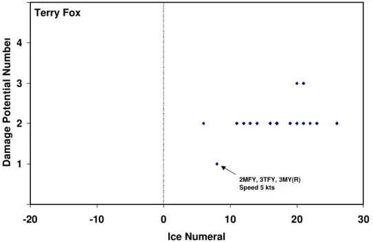
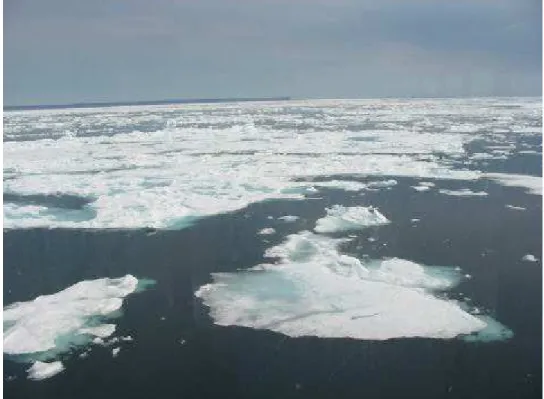
Figure 10 shows the Damage Potential versus the Ice Numeral using data from the Terry Fox. In virtually all of the events reported by the Terry Fox, the ice regimes were assessed to have the potential to damage the vessel. There was one regime that was identified as having a high potential for damage – 2/10 MFY, 3/10 TFY and 3/10 ridged MY ice. Figure 11 shows a photograph of the ice regime. Note that there was considerable ponding on the ice making the identification of the ice types difficult. The vessel speed in this ice regime was 5 knots.

Figure 12 shows the Damage Potential versus the speed of the vessel. There is no particular trend in the data.

Figure 13 shows the Ice Numeral versus the speed of the vessel. Similar to the Louis S. St-Laurent, there were no negative Ice Numerals for the Terry Fox.

The data from the Terry Fox are puzzling. The fact that most ice regimes were identified as having the potential to cause damage suggests to the authors that there was some confusion on this point. There were a number of comments in the Field Books that suggested that the rating was done for vessels being escorted by the Fox, and not for the Fox itself. The question of damage pertained to the Terry Fox, not the escorted vessel. This question should be phrased more clearly in future data collection programs.

(25)

0 1 2 3 4 5 -20 -10 0 10 20 30 Ice Numeral

Terry Fox

2MFY, 3TFY, 3MY(R) Speed 5 kts

Figure 10: Damage potential number versus the Ice Numeral for the Terry Fox.

Figure 11: Photograph of the ice regime (2/10 MFY, 3/10TFY & 3/10 ridged MY ice) rated as having a high potential for damage for the Terry Fox. Note that the ponding makes identification of the ice types difficult.

(26)

0 5 10 15 20 0 1 2 3 4 5

Terry Fox

Figure 12: Vessel speed versus the damage potential for the Terry Fox.

0 5 10 15 20 -20 -10 0 10 20 30 Ice Numeral

Terry Fox

(27)

Figure 14: Ice regime with 1/10 FY, 1/10 MFY, 5/10 TFY & 2/10 MY ice observed from the Terry Fox.

Figure 15: Ice regime with 5/10 MFY, 4/10 TFY & 1/10 MY ice observed from the Terry Fox.

(28)

Figure 16: Ice regime with ridged and decayed 2/10 MFY & 4/10 TFY ice observed from the Terry Fox.

Figure 17: Ice regime with 5/10 TFY & 1/10 ridged and decayed MY ice observed from the Terry Fox.

(29)

Figure 18: Ice regime with 1/10 N, 2/10 MFY, 3/10 TFY and 1/10 ridged MY ice observed from the Terry Fox.

Figure 19: Ice regime with 7/10 TFY and 1/10 ridged MY ice observed from the Terry Fox.

(30)

5.0 CCGS HENRY LARSEN

The HENRY LARSEN was built in 1987 and is designated as a Medium Gulf Icebreaker. Some salient details of this icebreaker are given in Table 8. Capts. J. Vanthiel and J. Broderick were the Commanding Officers. S. Payment and K. Carlson were the ISS personnel onboard. Data were collected from July 14 to September 9. Figure 2 shows the location of the vessel during the data collection timeframe. Observations were made in Foxe Basin, Gabriel Strait and the entrance to Frobisher Bay. Seven ice regime observations were reported as summarized in Table 9.

Table 8: Information on the CCGS HENRY LARSEN

CCGS HENRY LARSEN

Official No: 808731

Type: Medium Gulf - River

Icebreaker

Port of Registry:

Ottawa

Region: Newfoundland

Home Port: St. John's, Nfld.

Call Sign: CGHL

When Built: 1987

Builder: Versatile Pacific Shipyards Inc., Vancouver, B.C.

Modernized:

1 14-Jul 19-Jul J. Vanthiel S. Payment 3 3

2 19-Aug 9-Sep J. Broderick K. Carlson 4 4

(31)

Table 9: Summary of the Ice Regimes for the Henry Larsen

Speed

0 0 0 0 0 2 0 0 Y - - - 9 22 30 4 Lots of rubble and ridge remnants. 0 0 0 0 0 9 0 0 Y - - - 29 30 4

Rubble field with lots of ridge remnants. Some drainage on some of the larger small floes, but generally the floes are too small to have extensive drainage.

0 0 0 0 0 4 0 0 - - - 6 20 30 4 Rubble field with lots of ridge remnants. 0 0 0 0 0 1 0 0 Y - - - 9 21 30 2 0 0 0 0 0 1 0 0 Y - - - 7 21 30 2 0 0 0 0 0 1 0 0 Y - - - 7 21 30 2 0 0 0 0 0 3 0 0 Y - - - 7 23 30 2 CCG Comments DP #

Figure 20 shows the Damage Potential versus the Ice Numeral using data from the Henry Larsen. The data showed two different aspects. Three of the observations from one crew indicated that the ice regimes identified were unlikely to cause damage to the vessel. The second set (recorded by a different crew) indicated that all four observations had potential to damage the vessel. In all cases, the ice regimes were quite light, typically 1/10 to 3/10 decayed Thick First-year ice. Similar to the observations on the Terry Fox, there could have been confusion regarding the damage question.

Figure 21 shows the Damage Potential versus the speed of the vessel. There is no trend in the data. All of the speeds recorded were less than 10 knots. Figure 22 shows the Ice Numeral versus the speed of the vessel. No negative Ice Numerals were calculated for this vessel.

Figure 23 and Figure 24 show some examples of the ice regimes observed from the Henry Larsen. 0 1 2 3 4 5 -20 -10 0 10 20 30 Ice Numeral

Henry Larsen

Figure 20: Damage Potential Number versus the Ice Numeral for the Henry Larsen.

(32)

0 5 10 15 20 0 1 2 3 4 5

Henry Larsen

Figure 21: Vessel speed versus the Damage Potential Number for the Henry Larsen. 0 5 10 15 20 -20 -10 0 10 20 30 Ice Numeral

Henry Larsen

(33)

Figure 23: Ice regime with 9/10 TFY observed from the Henry Larsen.

(34)

6.0 CCGS DES GROSEILLIERS

The DES GROSEILLIERS was built in 1982 and is designated as a Medium Gulf Icebreaker. Some salient details of this icebreaker are given in Table 10. For these trials, Capts. G. Tremblay and R. Dubois were the Commanding Officers. B. Simard, S. Leger and E. Vaillant were the ISS personnel onboard. Data were collected from July 12 to September 19. Figure 2 shows the route for the vessel during the data collection timeframe. Fifty-seven ice regime observations were reported, most of which were made in Pelly Bay, Strathcona Sound, Norwegian Bay, Eureka Sound and Prince Regent Sound. They are summarized in Table 11.

Table 10: Information on the CCGS DES GROSEILLIERS

CCGS DES GROSEILLIERS

Official No: 802160

Icebreaker

Port of Registry:

Ottawa

Region: Laurentian

Home Port: Québec, Qué.

Call Sign: CGDX

When Built: 1982

Builder: Port Weller Dockyard, St. Catherines, Ont.

Modernized:

Ice Class: Crew: 26

MARPOL: Total: 38

IMO: Crewing Regime: Conventional

1 12-Jul 4-Aug G. Tremblay B. Simard 30 64

2 15-Aug 19-Sep R. Dubois S. Leger 27 40

(35)

Table 11: Summary of the Ice Regimes for the Des Groseilliers.

Speed

N G GW F Y MFY TFY SY MY FY SY MY FY SY MY Knots AIRSS Summer 0 0 0 0 2 1 0 0 - - - 1 19 29 3 0 0 0 0 1 2 0 0 - - - 3 18 28 4 0 0 0 0 3 1 0 0 Y - - - 11 23 29 4 0 0 0 0 0 3 0 0 Y - - - 1 20 27 3 0 0 0 0 1 6 0 1 Y - Y - - - 0.5 17 19 3 0 0 0 0 6 0 0 0 - - - 8 20 30 4 0 0 0 0 0 2 0 0 - - - 4 18 28 3 0 0 0 0 0 1 0 0 - - - 11 19 29 3 0 0 0 0 0 2 0 0 Y - - - 6 20 28 3 0 0 0 0 0 0 0 0 - - - 12 20 30 4 0 0 0 0 0 1 0 0 - - - Y - - 3 18 28 0 0 0 0 0 1 0 0 - - - 6 19 29 0 0 0 0 0 7 0 0 - - - 3 13 23 0 0 0 0 0 3 0 0 - - - 4 17 27 Multi-year floe. 0 0 0 0 0 1 0 0 - - - 10 19 29 3

0 0 0 0 1 3 0 1 Y - - - 10 16 21 2 The vessel in the photo is the Lady Franklin, waiting to be escorted. 0 0 0 1 1 2 0 2 Y - - - - Y 8 10 14 3 0 0 0 0 1 2 0 5 - - - Y - - 6 -10 -5 3 0 0 0 0 2 0 0 6 - - - Y 3 -16 -12 3 1 0 0 0 1 6 0 1 - - - Y - - 1 10 3 0 0 0 0 0 1 0 0 - - - 8 19 29 4 0 0 0 0 1 5 0 1 - - - 10 19 3 0 0 0 0 0 6 0 1 Y - Y - - - 5 16 19 3 0 0 0 0 0 5 0 0 Y - - - 7 20 25 2 0 0 0 0 1 6 0 1 Y - Y - - - 4 17 19 2 0 0 0 0 0 2 0 1 Y - Y - - - 7 16 23 3 1 0 0 0 1 6 0 1 Y - Y - - - 17 19 2 0 0 0 0 1 1 0 1 Y - Y - - - 9 17 24 3 0 0 0 0 1 1 0 1 Y - Y - - - 7 17 24 3 0 0 0 0 0 1 0 0 - - - 12 19 29 4 0 0 0 0 0 0 0 0 - - - 14 20 30 3 0 0 0 0 7 0 0 0 Y - - - 12 27 30 4 0 0 0 0 1 0 0 0 Y - - - 10 21 30 4 0 0 0 0 0 1 0 1 Y - Y - - - 12 16 24 4 0 0 0 0 0 8 2 0 Y Y - - - - 6 14 14 4 1 0 0 0 7 0 0 0 Y - - - 12 27 30 3 0 0 0 0 0 1 9 0 Y Y - - - - 10 -7 -7 3

- 4 motors / 6 motors in line

- Ice was mostly melted, causing little resistance to the vessel.

- The most important ice pieces (iceberg fragments) were easily detectable (good visibility) 0 0 0 0 0 3 6 0 Y Y - - - - 14 2 3 4 Proceed with 4 motors, full ahead

0 0 0 0 0 3 6 1 - - - 15 -12 -9 2 0 0 0 0 0 2 7 1 - - - 15 -15 -13 3 0 0 0 0 0 2 8 0 Y Y - - - - 6.5 -4 -4 2

0 0 0 0 0 2 6 0 Y Y - - - - 8.5 2 4 3 Proceed full ahead with 5 motors.

Average speed of 9.5 knts for first 2 hours of watch.

0 0 0 0 0 0 9 0 - Y - - - - 8 -7 -6 3 The vessel proceeds with 5 of 6 engines. Had to make 2 tries and go backwards because the vessel was immobilised due to the ice. Average speed of 6 knots in last 2 hours of watch. 0 0 0 0 0 3 6 0 Y Y - - - - 10 2 3 3

0 0 0 0 0 3 4 2 Y Y - - - - 9 -2 -1 4 CAC 4 for R class is too low. We should have the same as for the Henry Larsen (CAC 3). 0 0 0 0 0 1 1 1 Y Y - - - - 14 12 19 2

The previous night the vessel travelled in decayed SY ice with an IN of -13. The vessel proceeded without problem and the more severe ice was easy to detect. This morning there were ice pieces of different stages of decay.

4 0 0 0 0 4 0 1 Y - - - 10 15 20 4 For a vessel of this class, normal or decayed nilas ice doesn't make a difference _{in the movement of the vessel.} 0 0 0 0 0 2 0 2 Y - - - 9 10 16 3 Full ahead at 13 knots, with 4 of 6 motors.

0 0 0 0 0 2 0 1 Y - - - 6 15 22 3 Full ahead with 4 motors. 0 0 0 0 0 2 0 1 - - - Y - - 12 11 20 3

0 0 0 0 0 7 0 1 Y - Y Y - - 7 9 11 3

2 0 0 0 0 2 0 0 Y - - Y - - 11 16 24 4 Maneuver easily around large ice pieces. Very little speed reduction necessary 0 0 0 0 0 2 0 2 - - - 11 8 16 4 Easy progress, no speed reduction necessary.

0 0 0 0 0 1 0 1 - - - 10 14 23 2

2 0 0 0 0 6 0 1 Y - - - 6 15 18 4 Average speed between 16:00 and 17:00 was 11.5 knts. Proceeding with 4 motors. 0 0 0 0 0 8 0 2 - - - Y - Y 6 -8 0 Some drainage.

0 0 0 0 0 4 0 0 Y - - - 8 20 26 2

DP # CCG Comments

Figure 25 shows the Damage Potential versus the Ice Numeral using the data from the Des Groseilliers. No ice regimes were identified to have a high potential for damage for this vessel although nine events were identified to have a potential for damage. Two of these had a negative Ice Numeral whereas the other seven had a positive Ice Numeral. Further, there were a number of ice regimes that had a negative Ice Numeral yet were not deemed to be hazardous to the Des Groseilliers. A large number of these events occurred when the vessel traversed decayed Second-year ice, sometimes at speeds up to 15 knots.

(36)

Figure 26 shows the Damage Potential versus the speed of the vessel for the Des Groseilliers. There is no clear trend evident in the plot. There was a wide range of speeds regardless of the identified potential for damage.

Figure 27 shows the Ice Numeral versus the speed of the vessel. There is not a strong correlation between the vessel speed and the Ice Numeral. In a few cases, the vessel was travelling at speeds up to 15 knots in ice regimes with high concentrations of decayed Second-year ice (see Figure 28). There is an interesting comparison for this ice regarding damage potential. In one event, the ice regime consisted of 8/10 decayed Second-year ice and 2/10 decayed Thick First-year ice. In this case, the ice regime was noted to have a Potential for Damage. Another ice regime consisted of 1/10 Multi-year ice, 7/10 Second-year ice and 2/10 First-Second-year ice. This ice regime, although it was more severe than the previous ice regime, was said unlikely to damage the vessel. Two different Officers of the Watch rated these ice regimes.

Figure 28 to Figure 31 show some of the ice regimes observed from the Des Groseilliers.

0 1 2 3 4 5 -20 -10 0 10 20 30 Ice Numeral

Des Groseilliers

Figure 25: Damage Potential Number versus the Ice Numeral for the Des Groseilliers.

(37)

0 5 10 15 20 0 1 2 3 4 5

Figure 26: Vessel speed versus the Damage Potential Number for the Des Groseilliers. 0 5 10 15 20 -20 -10 0 10 20 30 Ice Numeral

(38)

Figure 28: Photograph of 2/10 decayed TFY and 8/10 decayed SY ice observed from the Des Groseilliers in Norwegian Bay.

(39)

Figure 30: Ice regime with 6/10 N and 2 TFY ice observed from the Des Groseilliers.

(40)

7.0 CCGS PIERRE RADISSON

The PIERRE RADISSON was built in 1978 and is designated as a Medium Gulf Icebreaker. Some salient details of this icebreaker are given in Table 12. Capts. M. Bourdeau and S. Brûlé were the Commanding Officers. R. Boisvert and F. Guay were the ISS personnel onboard. Data were collected from June 29 to October 17. Figure 2 shows the route for the vessel during the data collection timeframe. Most of the observations were made in Hudson Strait, Ungava Bay, Labrador Sea and Frobisher Bay. Forty-three ice regime observations were reported. Table 13 summarizes the ice regimes encountered by the Pierre Radisson.

Table 12: Information on the CCGS PIERRE RADISSON

CCGS PIERRE RADISSON

Official No: 383326

Icebreaker

Port of Registry:

Ottawa

Region: Laurentian

Home Port: Québec, Qué.

Call Sign: CGSB

When Built: 1978

Builder: Burrard Dry Dock Co. Ltd, North Vancouver, B.C.

Modernized: 1995, 1996, & 1997

Ice Class: 100 A Crew: 26

IMO: 7510834 Crewing Regime: Conventional

1 29-Jun 9-Jul M. Bourdeau R. Boisvert 18 15

2 14-Aug 11-Sep S. Brûlé F. Guay 14 29

(41)

Table 13: Summary of the Ice Regimes for the Pierre Radisson.

Speed

N G GW FY MFY TFY SY MY FY SY MY FY SY MY Knots AIRSS Summer 0 0 0 0 0 0 0 0 - - - 12 20 20 4 0 0 0 0 5 4 0 1 - - - 5 11 20 3 0 0 0 0 1 4 0 0 - - - 6 16 26 3 0 0 0 0 9 0 0 0 Y - - - 15 29 30 4 0 0 0 0 9 0 0 0 Y - - - 29 30 4 0 0 0 0 9 0 0 0 Y - - - 29 30 4 0 0 0 0 9 0 0 0 Y - - - 29 30 4 0 0 0 0 1 4 0 0 - - - 8 16 26 3 0 0 0 0 1 6 0 1 - - - 4 9 18 2 0 0 0 0 1 7 0 1 - - - 5 8 17 2 0 0 0 0 2 6 0 1 Y - Y - - - 3 18 19 2 0 0 0 0 0 10 0 0 - - - 2.5 10 20 2 0 0 0 0 0 4 0 0 - - - 5 16 26 3 0 0 0 0 0 0 0 0 - - - 12 20 30 4 0 0 0 0 0 8 0 1 - - - 3 7 16 2 0 0 0 0 4 0 0 1 Y - Y - - - 8 20 25 3 0 0 0 0 0 4 0 1 - - - 5 11 20 4 0 0 0 0 0 7 0 2 - - - 1 3 11 2

0 0 0 0 0 7 0 1 Y - Y - - - 7.8 16 18 4 Some melting and drainage. Very few ridges. 0 0 0 0 2 2 0 0 Y - - - 22 28 4 0 0 0 0 0 6 0 2 Y - Y Y - Y 4 6 4 0 0 0 0 3 6 0 0 Y - - - 23 24 4 0 0 0 0 1 1 0 0 Y - - - 21 29 4 0 0 0 0 0 1 0 0 Y - - - 20 29 3 0 0 0 0 0 1 0 0 Y - - - 20 29 4 0 0 0 0 0 6 2 1 Y Y Y Y Y Y 1 2 3 0 0 0 0 2 4 2 1 Y Y Y Y Y Y 2 3 4 2

Some decayed ice. 50% of the FY ice is decayed. TFY: 3 pieces with size 3 to 3.5 km (radar). TFY and MFY ice have some ridges, and are decayed about 75%.

0 0 0 0 0 3 4 3 - - - Y Y Y -24 -21 2

Although a bit far, the photos show a vast floe (2.6 x 2.5 nm by radar) of a "dangerous" looking piece of ice. Never saw anything so ridged before. Photo IMG_1031 shows the end of a long ridge line, approx. 15 feet height.

0 0 0 0 1 4 0 1 - - - Y - Y 10 5 14 2 Photos IMG_0481 to 0484 show a panoramic view of a multiyear floe (size 5).

3 0 0 0 3 1 0 1 Y - - - 5 18 23 4 MFY and TFY ice are rotten/decayed.

0 0 0 0 0 1 0 1 - - - Y - Y 13 12 21 4 No melt. Water temperature: -1.3 deg C. Air temperature: _{-4.0 deg C.} 3 0 0 0 2 2 0 3 - - - Y - Y 4.5 -7 0 2

1 0 0 0 0 4 1 4 - - - 5 -8 -3 2 Ice is reforming and ponds are freezing back 0 0 0 0 0 3 0 7 - - - 5 -18 -15 2 0 0 0 0 0 3 0 7 - - - 5 -18 -15 1 7 0 0 0 0 0 0 0 - - - 10 20 20 3 9 0 0 0 0 0 0 0 - - - 9 20 20 3 0 1 5 0 0 2 0 0 - - - 6 18 18 3 1 2 3 0 0 0 1 1 - - - 8 11 11 3 10 0 0 0 0 0 0 0 - - - 10 20 20 4 0 2 8 0 0 0 0 0 - - - 10 20 20 4 0 0 2 0 0 0 4 4 - - - 4 -16 -16 1 1 0 6 0 0 0 1 0 - - - 8 16 16 3 DP # CCG Comments Ice Concentration Decay Ridged Ice Numeral

Figure 32 shows the Damage Potential versus the Ice Numeral using data from the Pierre Radisson. Two ice regimes were identified to have a high potential for damage. The first ice regime consisted of 3/10 Thick First-year ice and 7/10 Multi-year ice (see Figure 33). The Ice Numeral for this regime was –18. The speed of the Radisson was 5 knots in this ice. The Second ice regime consisted of 2/10 Grey-White ice, 4/10 Second-year ice and 4/10 Multi-year ice (Figure 34). The Ice Numeral was –16. The speed of the Radisson in this ice regime was 4 knots.

(42)

0 1 2 3 4 5 -20 -10 0 10 20 30 Ice Numeral

Pierre Radisson

2GW,4SY,4MY Speed 4 kts 3TFY,7MY

Speed 5 kts

Figure 32: Damage Potential Number versus the Ice Numeral for the Pierre Radisson.

Figure 33: Photograph of 3/10 Thick First-year ice and 7/10 Multi-year ice. This ice regime was identified to have a high potential for damage for the Pierre Radisson. The Ice Numeral for this ice regime for a CAC4 vessel is -18.

(43)

Figure 34: Photograph of 2/10 Grey-White ice, 4/10 Second-year ice and 4/10 Multi-year ice. This ice regime was identified to have a high potential for damage for the Pierre Radisson. The Ice Numeral for this ice regime for a CAC4 vessel is -16.

Figure 35 shows the Damage Potential versus the speed of the vessel. There is a trend of decreasing speed as the perceived damage potential increased (i.e. the DP number gets smaller). This trend makes physical sense.

Figure 36 shows the Ice Numeral versus the speed of the vessel. The graph shows lower speeds for negative Ice Numerals.

Data from the Pierre Radisson were very consistent. The identification of the ice regimes and their damage potential were reflected in the vessel speed and the assessment of the ice regimes.

(44)

0 5 10 15 20 0 1 2 3 4 5

Pierre Radisson

Figure 35: Vessel speed versus the Damage Potential Number fro the Pierre Radisson. 0 5 10 15 20 -20 -10 0 10 20 30 Ice Numeral

Pierre Radisson

Figure 36: Vessel speed versus the Ice Numeral for the Pierre Radisson. Note the lower speeds with the negative Ice Numerals.

(45)

Figure 37: Ice regime with 9/10 decayed MFY ice observed from the Pierre Radisson.

(46)

Figure 39: Ice regime with decayed 3/10 MFY and 6/10 TFY ice observed from the Pierre Radisson.

Figure 40: Ice regime with 3/10 N, decayed 3/10 MFY& 1/10 TFY, & 1/10 MY ice observed from the Pierre Radisson.

(47)

Figure 41: Ice regime with 3/10 TFY and 7/10 MY ice observed from the Pierre Radisson.

Figure 42: Ice regime with 1/10 N, 2/10 G, 3/10 GW, 1/10 SY and 1/10 MY ice observed from the Pierre Radisson.

(48)

8.0 CCGS SIR WILFRID LAURIER

The SIR WILFRID LAURIER was built in 1986 and is designated as a Light Icebreaker. Some salient details of this icebreaker are given in Table 14. Capts. M. Taylor and N. Thomas were the Commanding Officers. S. Thompson, C. Stock and C. Daigle were the ISS personnel onboard. Data were collected from July 19 to August 25. Figure 2 shows the location for the vessel during the data collection timeframe. Observations were made off Barrow, Smith Bay, Cape Parry, Victoria Strait and Larsen Sound. Thirteen ice regime observations were reported and these are summarized in Table 15.

Table 14: Information on the CCGS SIR WILFRID LAURIER

CCGS SIR WILFRID LAURIER

Official No: 807038

Type: Light Icebreaker - Major

Navaids Tender

Port of Registry:

Ottawa

Region: Pacific

Home Port: Victoria, B.C.

Call Sign: CGJK

When Built: 1986

Builder: Canadian Shipbuilding, Collingwood, Ont.

Modernized:

1 19-Jul 3-Aug M. Taylor S. Thompson 9 0

2 16-Aug 25-Aug N. Thomas C. Stock 4 26

(49)

Table 15: Summary of the Ice Regimes for the Sir Wilfrid Laurier.

Speed

0 0 0 0 0 5 0 0 - - - 5 15 0 0 0 0 0 9 0 0 - - - -7 3 0 0 0 0 0 4 0 0 Y - - - 5.2 12 18 4 0 0 0 0 0 4 0 0 Y - - - 12 18 0 0 0 0 1 5 0 0 Y - - - 10 14 0 0 0 0 3 3 0 1 Y - Y - - - 5 9 12 0 0 0 0 3 4 0 1 Y - Y - - - 5 7 9 0 0 0 0 0 5 0 0 Y - - - 7 10 15 0 0 0 0 1 3 0 1 Y - Y - - - 5 9 14 0 0 0 1 6 1 0 0 Y - - - 6 19 21 4

- Northbound through Victoria Strait, enroute Peel Sound for rendez-vous with cruise ship 'Hanseatic'

- Predominantly medium and thin FY ice showing significant degradation and melt

- Thick FY in concentrations from trace amounts to 1/10

0 0 0 3 4 1 0 0 Y - - - 4.6 21 23 3

- Northern reaches of Victoria Strait - Trace amts of SY ice and ridges - Significant melt and rot

0 0 0 1 5 2 0 0 Y - - - 7 17 19 4

- Escort of M/V Hanseatic southwards through Larsen Sd and Victoria Strait

- Level, decayed MFY ice

- No pressure, coming through ice edge.

0 0 0 0 0 9 0 0 - - - Y - - 2 -16 -6 1

- Ship escorting M/V Hanseatic westwards towards Herschel Island (visibility reduced in fog throughout day).

- Predominantly thick FY ice showing normal summer melt. Ridge remnants of old ice in small floes.

- This was a significant ice field, and extr

DP # CCG Comments

Figure 43 shows the Damage Potential versus the Ice Numeral using the data from the Sir Wilfrid Laurier. A number of the observed ice regimes were not evaluated in terms of their damage potential, but those that were evaluated were quite consistent. There was one ice regime that was identified as having a high potential for damage for this vessel. That ice regime consisted of 9/10 ridged First-year ice with ponding (see Figure 44). The Ice Numeral for this ice regime for a Type A vessel is –16. The speed of the vessel was 2 knots.

Figure 45 shows the Damage Potential versus the speed of the vessel. There is a trend of lower speeds in ice regimes that are identified as having a high damage potential.

Figure 46 shows the Ice Numeral versus the speed of the vessel. The ice regime with a negative Ice Numeral had a low speed of 2 knots.

In general, the data from the Sir Wilfrid Laurier were quite consistent. Unfortunately, not all of the ice regimes identified were rated in terms of their damage potential. In addition, although there were photographs of the ice regimes, the photo names were not always indicated in the Field Book. This made it difficult to correlate the photos to the ice regimes.

Figure 47 and Figure 48 show some of the ice regimes observed from the Sir Wilfrid Laurier.

(50)

0 1 2 3 4 5 -20 -10 0 10 20 30 Ice Numeral

Sir Wilfrid Laurier

9TFY(R) Speed 2 kts

Figure 43: Damage Potential Number versus the Ice Numeral for the Sir Wilfrid Laurier.

Figure 44: Photograph of 9/10 ridged Thick First-year ice as observed from the Sir Wilfrid Laurier. The Ice Numeral for this ice is –16 for a Type A vessel.

(51)

0 5 10 15 20 0 1 2 3 4 5

Figure 45: Vessel speed versus the Damage Potential Number for the Sir Wilfrid Laurier. 0 5 10 15 20 -20 -10 0 10 20 30 Ice Numeral

9TFY(R) Speed 2 kts

(52)

Figure 47: Ice regime with decayed 1/10 FY, 6/10 MFY & 1/10 TFY ice observed from the Sir Wilfrid Laurier.

Figure 48: Ice regime with decayed 3/10 FY, 4/10 MFY & 1/10 TFY ice observed from the Sir Wilfrid Laurier.

(53)

9.0 GENERAL ANALYSIS

The data obtained from this study can be used to investigate several aspects of the Ice Regime System. An analysis of the data is provided in the following sections.

9.1 Calculating the Ice Numeral

The data collection project showed that defining ice regimes and calculating the Ice Numeral was not a problem. Figure 49 shows the overall breakdown of the calculated Ice Numeral for the 201 events. In 72% of the cases, the Ice Numeral was calculated correctly based upon the observed ice regime. However, three different types of mistakes were made:

§ The Open Water was not included in the ice regime in 16% of the cases. Since the

Open Water Ice Multiplier is +2 for all vessels, this led to an overly negative Ice Numeral for those ice regimes. This was done consistently by a few of the ISS personnel, and this skews the data towards a larger number of incorrect Ice Numerals.

§ The wrong Ice Multiplier was used in 9% of the cases. For example, the ice

regime was identified as having decayed ice, but the decay bonus of +1 was not applied to the Ice Multiplier.

§ In 3% of the cases, mistakes were made summing the contributions from each ice

type when determining the Ice Numeral (i.e. arithmetic errors).

These results are encouraging despite the errors in determining the Ice Numeral in about one-quarter of the observations. The program shows that determining the Ice Numeral is relatively straightforward once the ice regime has been defined. The mistakes of neglecting the Open Water and incorrect summing can be corrected by taking a more careful approach. The mistake of choosing the incorrect Ice Multiplier would be remedied with more experience with the Ice Regime System.

Ice Numeral calculated correctly 72% Incorrect Ice Concentration 1% Open Water not taken into account 16% Arithmetic error 2% Decay not taken into account 8% Incorrect Ice Multiplier used 1%