HAL Id: hal-02440789
https://hal.archives-ouvertes.fr/hal-02440789
Submitted on 15 Jan 2020
HAL is a multi-disciplinary open access
archive for the deposit and dissemination of sci-entific research documents, whether they are pub-lished or not. The documents may come from teaching and research institutions in France or abroad, or from public or private research centers.
L’archive ouverte pluridisciplinaire HAL, est destinée au dépôt et à la diffusion de documents scientifiques de niveau recherche, publiés ou non, émanant des établissements d’enseignement et de recherche français ou étrangers, des laboratoires publics ou privés.
Zhenzhong Zeng, Alan Ziegler, Timothy Searchinger, Long Yang, Anping
Chen, Kunlu Ju, Shilong Piao, Laurent Li, Philippe Ciais, Deliang Chen, et al.
To cite this version:
Zhenzhong Zeng, Alan Ziegler, Timothy Searchinger, Long Yang, Anping Chen, et al.. A reversal in global terrestrial stilling and its implications for wind energy production. Nature Climate Change, Nature Publishing Group, 2019, 9 (12), pp.979-985. �10.1038/s41558-019-0622-6�. �hal-02440789�
A reversal in global terrestrial stilling and its implications for wind energy
1production
2Zhenzhong Zeng1,2*, Alan D. Ziegler3, Timothy Searchinger4, Long Yang5, Anping Chen6,
3
Kunlu Ju7, Shilong Piao8, Laurent Z. X. Li9, Philippe Ciais10, Deliang Chen11, Junguo Liu2, Cesar
4
Azorin-Molina11,12, Adrian Chappell13, David Medvigy14, Eric F. Wood1
5
1 Department of Civil and Environmental Engineering, Princeton University, Princeton, New
6
Jersey 08544, USA
7
2 School of Environmental Science and Engineering, South University of Science and
8
Technology, Shenzhen 518055, China
9
3 Geography Department, National University of Singapore, 1 Arts Link Kent Ridge, Singapore
10
117570, Singapore
11
4 Woodrow Wilson School, Princeton University, Princeton, New Jersey 08544, USA
12
5 School of geography and ocean science, Nanjing University, Nanjing, Jiangsu Province, China
13
6 Forestry and Natural Resources, Purdue University, West Lafayette, Indiana 47907, USA
14
7 School of Economics and Management, Tsinghua University, Beijing 100084, China
15
8 Sino-French Institute for Earth System Science, College of Urban and Environmental Sciences,
16
Peking University, Beijing 100871, China
17
9 Laboratoire de Météorologie Dynamique, CNRS, Sorbonne Université, Ecole Normale
18
Supérieure, Ecole Polytechnique, 75252 Paris, France
19
10 Laboratoire des Sciences du Climat et de l’Environnement, UMR 1572 CEA-CNRS-UVSQ,
20
91191 Gif-sur-Yvette, France
21
11 Regional Climate Group, Department of Earth Sciences, University of Gothenburg,
22
Gothenburg, Sweden
23
12 Centro de Investigaciones sobre Desertificación, Consejo Superior de Investigaciones
24
Cientificas (CIDE-CSIC), Montcada, Valencia, Spain
25
13 School of Earth and Ocean Sciences, Cardiff University, Wales, CF10 3AT, UK
26
14 Department of Biological Sciences, University of Notre Dame, Notre Dame, IN 46556, USA
27
*Correspondence to: zzeng@princeton.edu
28 29
Manuscript for Nature Climate Change
30
September 01, 2019
31 32
Wind power, a rapidly growing alternative energy source, may be threatened by reductions 33
in global average surface wind speed over land since the 1980s, known as terrestrial stilling. 34
However, this stilling is largely unexplained so far. Here we use wind data from in-situ 35
stations worldwide to show that the stilling reversed around 2010 and global wind speeds 36
over land have recovered. We illustrate that decadal-scale variations of near-surface wind 37
are likely dertermined by internal decadal ocean/atmosphere oscillations, rather than the 38
previous hypothesis of vegetation growth and/or urbanization. The strengthening has 39
increased potential wind energy by 17 ±2% for 2010-2017, increasing U.S. wind power 40
capacity factor by ~2.5% that is as significant as technology innovations. In the longer-term, 41
use of ocean/atmosphere oscillations to anticipated future wind speeds, could allow 42
optimization of turbines for expected speeds during their productive life spans. 43
44
Reports of a global decline in land surface wind speed of 8% from ~1980 to 2010 have raised
45
concerns about outputs from future wind power1-5. Wind power (p) varies with the cube of wind
46
speed (u) according to the formula
47 3 2 sf p= u (1), 48
where is air density, s the swept area of the turbine, and
f
an efficiency factor6. The decline49
has been manifest in the northern mid-latitude countries where the majority of wind turbines are
50
installed including China, the U.S. and Europe1. If the observed trend from 1980 to 2010 were to
51
continue to the end of the century, global u would reduce by 21%, halving the amount of power
52
available in the wind (using Equation (1)). Understanding the drivers of this long-term decline in
53
wind speed is critical not merely to maximize wind energy production7-9 but also to address other
54
globally significant environmental problems related to stilling, including reduced aerosol
dispersal, changes in evapotranspiration rates, and adverse effects on animal behavior and
56
ecosystem functioning1,3,4,10.
57 58
The potential causes for global terrestrial stilling are complex and remain contested2,3,11,12. Many
59
regional-scale studies13-15G&W using reanalysis datasets have found correlations of u with various
60
climate indices. Those studies hypothesize that terrestrial stilling is caused by decreased driving
61
force due to the change in large scale circulations11. This is supported by a consistency in wind
62
speed changes at the surface and at higher levels in the reanalysis datasets11,14. Nevertheless,
63
there are large uncertainties in these datasets2,11,14, and more importantly, global terrestrial
64
stilling is either not reproduced or has been largely underestimated in global reanalysis
65
products2,11 (Supplementary Fig. 1) and/or climate model simulations for IPCC AR5
66
(Supplementary Fig. 2). Acknowledging that wind speed reanalysis datasets do not represent land
67
surface dynamics, the discrepancies between the decreasing trends derived from in-situ stations
68
and from reanalysis or climate model simulations lead to the hypothesis that global terrestrial
69
stilling is caused by increased drag related to increased surface roughness from the greening of
70
the Earth and/or urbanization2,16, both of which would suggest further future declines.
71 72
However, conversely, recent studies have described wind speed reversal at local scales17,18 or an
73
increase of global wind speed during a particular year19, despite uncertainty over the global trend
74
of wind speed change5,11. The recent reversal over land, if evidenced to be true at global scale,
75
could elucidate the causes of global terrestrial stilling and potentially improve future wind energy
76
projections.
77 78
Analysis 79
We integrate direct in-situ observations of u from ground weather stations from 1978 to 2017
80
together with statistical models for detection of trends. The stations, mainly distributed in the
81
northern mid-latitudes countries, were carefully selected from the Global Summary of Day
82
(GSOD) database following strict quality control procedures (Supplementary Fig. 3; see Methods
83
for details). To test for a continuation of the terrestrial stilling after 2010 (refs 1-3), we use a
84
piecewise linear regression model to examine the potential trend changes26,27.
85 86
Scope of a reversal in global terrestrial stilling 87
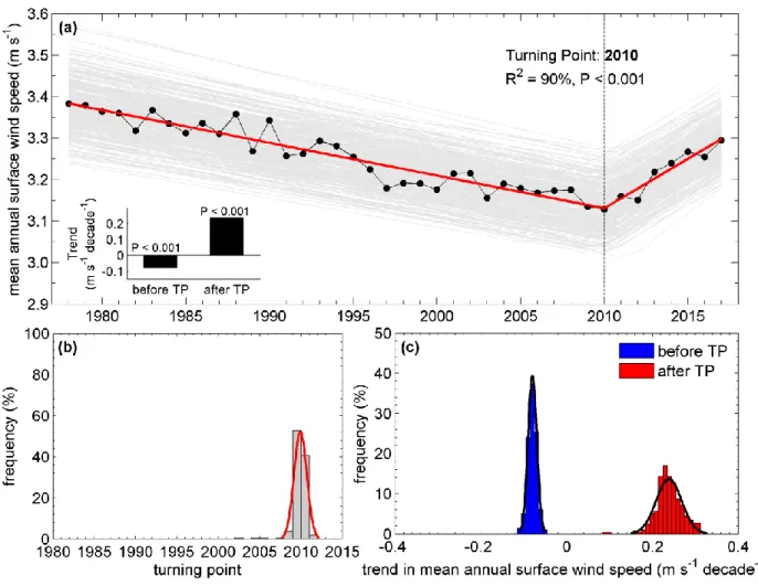
The analysis shows that global mean annual u decreased significantly at a rate of -0.08 m s-1 (or
-88
2.3%) per decade during the first three decades beginning in 1978 (P-value < 0.001; Fig. 1a,
89
Supplementary Table 1). While the decreasing trend has previously been shown2-4 and confirms
90
global terrestrial stilling as an established phenomenon during the period of 1978-2010, we find
91
that u has significantly increased in the current decade. This turning point is statistically
92
significant at P < 0.001 with a goodness of fit of an R2 = 90% (Fig. 1a). The recent increasing
93
rate of 0.24 m s-1 decade-1 (P < 0.001) is three-fold the decreasing rate before the turning point in
94
2010.
95 96
To exclude the possibility that the turning point is caused by large wind speed changes at only a
97
few sites, we repeat our analyses 300 times by randomly resampling 40% of the global stations
98
each time (grey lines in Fig. 1a; 40% of the stations are selected to ensure a sufficient sample
99
size (n > 500)). We find significant turning points in each randomly-selected sub-sample (P <
100
0.001; R2 ≥ 76%). Run-specific turning points occur between 2002 and 2011, with most (95%) of
them between 2009 and 2011 (Fig. 1b). In addition, mean annual u changes before and after a
102
specific turning point based on the 300 sub-sample estimates are -0.08 ± 0.01 m s-1 per decade
103
and 0.24 ± 0.03 m s-1 per decade, respectively (Fig. 1c), identical to those values based on all the
104
global samples.
105 106
Spatial analyses further confirm that the recent reversal is a global-scale phenomenon
107
(Supplementary Fig. 4a-c). A majority (79%) of the stations where u decreased significantly
108
during 1978-2010 (Supplementary Fig. 4b) have positive trends in u after 2010 (Supplementary
109
Fig. 4c). The stations are mainly distributed over North America, Europe, and Asia. Significant
110
turning points exist in all the three regional mean annual u time series (P < 0.001, Supplementary
111
Fig. 4d-f), but they vary in the specific year of occurrence. For example, a turning point occurs
112
earlier in Asia (2001, R2 =80%, Supplementary Fig. 4f) and Europe (2003, R2 = 56%,
113
Supplementary Fig. 4e) than in North America (2012, R2 = 80%, Supplementary Fig. 4d).
114
Nevertheless, all the three regions have the most significant increase in u after ~2010
115
(Supplementary Fig. 4d-f).
116 117
The existence of turning points is robust regardless of season (Supplementary Table 1 and
118
Supplementary Fig. 5) or wind variable chosen for analysis (Supplementary Fig. 6), and shows
119
no dependence on quality control procedures for weather station data (Supplementary Fig. 7).
120
For maximum sustained wind and wind gusts, the turning points appear earlier and the recent
121
increasing rates are weaker (Supplementary Fig. 6). Furthermore, we show that our findings are
122
robust and repeatable (Supplementary Fig. 8) using a different data set—the HadISD database,
123
which follows station selection criteria and a suite of quality control tests established by Met
Office Hadley Centre28. We also find that the tendency for an increasing number of stations
125
becoming automated during recent decades (Supplementary Figs 9 and 10) does not affect the
126
result (Supplementary Fig. 11). Finally, to test the effect of inhomogeneity, we remove all the
127
stations with change points detected by the Pettitt tests29, finding that the reults do not change
128
after the analysis is repeated (Supplementary Fig. 12). All these lines of evidences provide
129
independent supports that the trends in u are not caused by changes in measurement methods and
130
inhomogeneity.
131 132
Causes of the reversal in global terrestrial stilling 133
A variety of theories have been presented previously to explain stilling, many of which focus on
134
the drag force of u linked to increased terrestrial roughness caused by urbanization and/or
135
vegetation changes2,12. These theories have been disputed30 (also see Supplementary Figs 13 and
136
14). Our finding that global stilling changed after 2010, especially the increasing rate which is
137
three times that of the decreasing rate before 2010 (Fig. 1a), further refutes these theories
138
because terrestrial roughness did not suddenly change in 2010. More likely, the variation in u
139
(including prior stilling and the recent reversal) is determined mainly by driving forces
140
associated with decadal variability of large-scale ocean/atmospheric circulations.
141 142
Wind is physically created by pressure gradient which is due to uneven heating of the Earth
143
surface (temperature anomalies or heterogeneity), and the latter is to a large extent described by
144
climate indices for oscillations. To test such associations, we first include twenty-one climate
145
indices in the pool of indicators forocean/atmosphere oscillations (Supplementary Table 2 and
146
Methods). To avoid overfitting, we apply stepwise regression32 to identify six largest explanatory
power factors for the decadal variations of u over the globe, North America, Europe, and Asia,
148
respectively (see Supplementary Table 3). The reconstructed u obtained from the stepwise linear
149
regression matches well with the observed u (Supplementary Figs 15 and 16, and discussion in
150
Methods). Finally, we train our models only using the detrended time series before the turning
151
points (2010 for the globe, 2012 for North America, 2003 for Europe, and 2001 for Asia), finding
152
that the models are capable of reproducing the positive trends after the turning points, not only
153
for the globe (P < 0.001; Fig. 2a), but also for all the three regions (P < 0.001; Fig. 2b-d). The
154
magnitude of the increasing rate after the turning points is well modelled (Fig. 2). These results
155
suggest a predictive relationship between wind changes and ocean/atmosphere oscillations,
156
which would be very valuable for the wind energy sector.
157 158
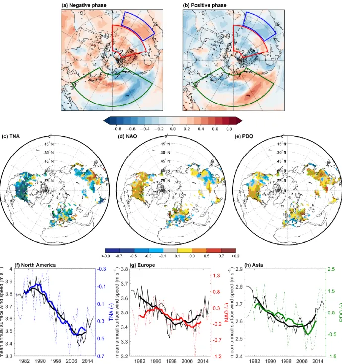
To uncover the mechanisms behind the decadal variations of u, we construct the composite
159
annual mean surface temperature for the years that exhibit negative (Fig. 3a) and positive (Fig.
160
3b) anomalies of detrended u. During the years of negative u anomalies (Fig. 3a) the following
161
are observed: (a) positive anomalies of temperature prevail over the Tropical Northern Atlantic
162
(TNA region, 5.5oN to 23.5oN, 15oW to 57.5oW), showing a positive value for Tropical Northern
163
Atlantic Index (TNA); (b) the west (east) Pacific is warmer (colder) than normal years,
164
demonstrating a negative value for Pacific Decadal Oscillation (PDO); and (c) positive anomalies
165
of temperature occur near the Azores and negative anomalies occur over Greenland, indicating a
166
negative value for North Atlantic Oscillation (NAO). The opposite pattern (i.e. negative TNA,
167
positive PDO and NAO) occurs during the years of positive u anomalies (Fig. 3b). Furthermore,
168
TNA has strong, significant, and negative correlations with regional u, in particular, over North
169
America (Fig. 3c). PDO has significant positive correlations with regional u globally (Fig. 3e).
NAO has overwhelmingly significant positive correlations with regional u in the U.S. and
171
Northern Europe, but negative correlation with regional u in Southern Europe (Fig. 3d). These
172
patterns are consistent with the finding that the greatest explanatory power factor is TNA for
173
North America (R = -0.67, P < 0.001), PDO for Asia (R = 0.50, P < 0.01), and NAO for Europe
174
(R = 0.37, P < 0.05) (more discussions refer to Methods). The ocean/atmosphere oscillations,
175
characterized as the decadal variations in these climate indices (mainly TNA, NAO, PDO), can
176
therefore explain the decadal variation of u (i.e., the long-term stilling and the recent reversal)
177
(Figs 2 and 3f-h).
178 179
There are some theories20-23 for potential physical mechanisms how these oscillations affect
180
regional u over land. With respect to TNA, prior studies demonstrate that the positive phase of
181
TNA is linked with a weakened Hadley circulation (more details refer to ref. 21). During the
182
positive phase of TNA there is a cold anomaly over the eastern coast of the U.S. (Fig. 3a and ref.
183
21). This pattern leads to a southward component of surface wind and a stable environment of
184
weak convergence from the tropics to the latitudes, resulting a reduction of u in the
mid-185
latitudes, the U.S. in particular (Fig. 3c and Supplementary Fig. 17a,b). As for NAO, its negative
186
and positive phases have different jet stream configurations and wind systems in Northern versus
187
Southern Europe (Supplementary Fig. 17c,d; details refer to ref. 20). During the positive
188
(negative) phase, the pressure gradient across the North Atlantic20 generates strong winds and
189
storms across Northern (Southern) Europe (Supplementary Fig. 17c,d), explaining the
190
contrasting correlations of NAO to u in Northern and Southern Europe (Fig. 3d, Supplementary
191
Fig. 18). For PDO, the temperature gradient during the negative (positive) phase generates an
192
easterly (westerly) component of surface wind (details refer to refs 22, 23), which weakens
(strengthens) the prevailing westerly winds in the mid-latitudes (Supplementary Fig. 17e,f) and
194
explains the widespread and significant positive correlations between PDO and u across the
195
whole mid-latitudes (Fig. 3e). However, despite these potential physical mechanisms20-23, the
196
relationships between these oscillations and long-term wind speeds over land are still uncertain
197
and require more investigations.
198 199
Finally, it is critical to determine why global reanalysis products do not reproduce or
200
underestimate the historical terrestrial stilling (Supplementary Fig. 1), which is a major basis for
201
the previous studies2,12 rejecting the ocean/atmosphere oscillations as a dominant driver for
202
terrestrial stilling. Global reanalysis products are generated at numerical weather prediction
203
centers with their most-advanced data assimilation systems. But most of them cannot properly
204
assimilate near-surface winds over land due to inappropriate model topography and inaccuarency
205
of atmospheric boundary layer processes implemented into the data assimilation systems.
ERA-206
Interim35, one of the best products available, can only assimilate surface winds over seas from
207
scatterometers, ships and bouys. The capacities of these products in reproducing the near-surface
208
wind speed over land are thus generally poor and rely on climate models. We find that in the
209
regions where AMIP model simulations (i.e. atmospheric simulations forced with observed sea
210
surface temperature) capture the stilling, such as Europe and India (Fig. 4a,b in ref. 30), the
211
global reanalysis products are also capable of reproducing the stilling in these regions (Fig. S1c);
212
while in regions where AMIP simulations do not capture the stilling, such as North America30,36,
213
the global reanalysis products also fail to reproduce the stilling2,11 (Fig. S1b). Therefore, it is the
214
model limitations that prevent global reanalysis products from reproducing the observed
near-215
surface wind speed changes in some regions satisfactorily. More efforts are required to improve
surface process parameterization scheme and its connection to ocean/atmosphere circulations in
217
climate models and operational weather data assimilation systems.
218 219
Implications for wind energy production 220
In wind power assessments, near-surface wind observations from weather stations (u at the
221
height of zr = 10 meters) are often used to estimate wind speeds at the height of a turbine (u at tb
222
the height of z = 50-150 meters) using an exponential wind profile power law relationship: tb
223 tb tb r z u u z = (2) 224
where the α is commonly assumed to be constant (1/7) in wind resource assessments because the
225
differences between these two levels are unlikely great enough to introduce considerable errors
226
in the estimates5.
227 228
Changes in wind speed matter not only on average but also in the percentage of time wind speeds
229
are high or low. A utb > 3 m s-1 is a typical minimum velocity needed to drive turbines efficiently,
230
so wind speeds below 3 m s-1 are typically wasted from the power generation perspective.
231
Although periods of high wind speed greatly increase the physical capacity to generate power
232
according to formula (1), turbines are built with a maximum capacity, so periods of high wind
233
speed can also “waste” the uses of wind with the threshold depending on the capacity of the
234
turbine.
235 236
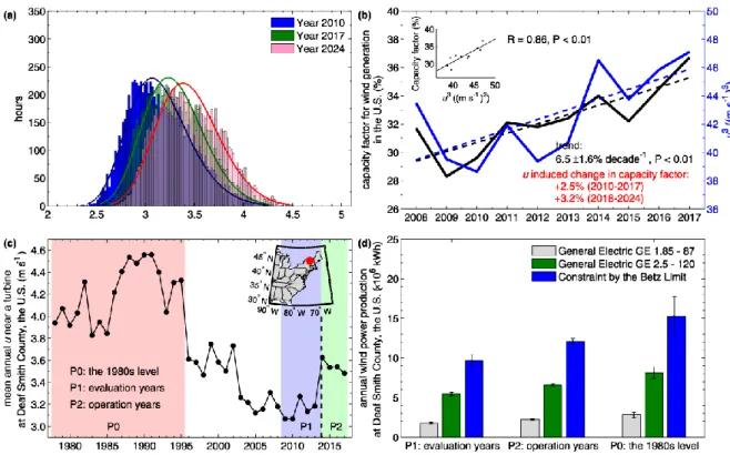
On average, the increase of global mean annual u from 3.13 m s-1 in 2010 to 3.30 m s-1 in 2017
237
(Fig. 1a; see Methods for details) increases the amount of energy entering a hypothetical wind
turbine receiving the global average wind by 17 ±2% (uncertainty is associated with subsamples
239
in Fig. 1a; regionally, 22 ±2% for North America, 22 ±4% for Europe, and 11 ±4% for Asia). At
240
the hourly scale, the frequency of low u decreases while the frequency of high u increases (Fig.
241
4a). Using one General Electric GE 2.5 – 120 turbine37 (Supplementary Fig. 19) to illustrate, the
242
effects of changes in global average u increase potential power generation from 2.4 million kWh
243
in 2010 to 2.8 million kWh in 2017 (+17%). If the present trend persists for at least another
244
decade, in the light of the robust increasing rate during 2000-2017 (Fig. 1a) and the long cycles
245
of natural ocean/atmosphere oscillations20-24 (Supplementary Fig. 20), power would rise to 3.3
246
million kWh in 2024 (+37%), resulting in a +3% per decade increase of global-average capacity
247
factor (mean power generated divided by rated peak power) on average. This change is even
248
larger than the projected change in wind power potential caused by climate change under
multi-249
scenairos38.
250 251
During the past decade, the capacity factor of the U.S. wind fleet39 has steadily risen at a rate of
252
+7% per decade (Fig. 4b), previously attributed solely to technology innovations40. We find that
253
the capacity factor for wind generation in the U.S. is highly and significantly correlated with the
254
variation in the cube of regional-average u (u3, R = 0.86, P < 0.01; Fig. 4b). To isolate the
u-255
induced increase in capacity factor from that due to technology innovations, we use the regional
256
mean hourly wind speed in 2010 and 2017 to estimate the increase of capacity factor for a given
257
turbine, thereby controlling for technology innovations. It turns out that the increased u3 explains
258
~50% of the increase of the capacity factor (see Methods for details). Therefore, in addition to
259
technology innovations, the strengthening u is another key factor powering the increasing
reliability of wind power in the U.S. (and other mid-latitude countries where u is increasing, such
261
as China and European countries).
262 263
To illustrate the consequences, one turbine (General Electric GE 1.85 – 87 (ref. 41)) installed at
264
one of our in-situ weather stations in the U.S. in 2014 (inset plot in Fig. 4c), which was expected
265
to produce 1.8 ±0.1 million kWh using four years of u records before the installation
(2009-266
2013)41, actually produced 2.2 ±0.1 million kWh between 2014-2017 (+25%). This system has
267
the potential to generate 2.8 ±0.1 million kWh (+56%) if u recovers to the 1980s level (red bars
268
in Fig. 4d; see Methods for details). Globally, 90% of the global cumulative wind capacity has
269
been installed in the last decade25, during which global u has been increasing (see above).
270 271
Discussion 272
Although the response of ocean/atmosphere oscillations to anthropogenic warming remains
273
unclear23, the increases in wind speeds should continue for at least a decade because these
274
oscillations change over decadal time frames20-24. Climate model simulations constrained with
275
historical sea surface temperature also show a long cycle in u over land (Supplementary Fig. 20).
276
Our findings are therefore good news for the power industry for the near future.
277 278
However, oscillation patterns in the future will likely cause returns to declining wind speeds, and
279
anticipating these changes should be important for the wind power industry. Wind farms should
280
be constructed in the areas with stable winds and high effective utilization hours (e.g. 3 - 25 m s
-281
1). If high wind speeds are likely to be common, building turbines with larger capacities could be
282
justified. For example, capturing more available wind energy (blue bars in Fig. 4d) could be
achieved through the installation of higher capacity wind turbines (e.g. General Electric GE 2.5 –
284
120, green bars in Fig. 4d), greatly increasing total power generation. Most turbines tend to
285
require replacement after 12-15 years42. Further refinement of the relationships uncovered in this
286
paper could allow choices of turbine capacity, rotor and tower that are optimized not just to wind
287
speeds of the recent past but to likely future changes during the lifespan of the turbines.
288 289
In summary, we find that after several decades of global terrestrial stilling, wind speed has
290
rebounded, increasing rapidly in the recent decade globally since 2010. Ocean/atmosphere
291
oscillations, rather than increased surface roughness, are likely the causes. These findings are
292
important for those vested in maximizing the potential of wind as an alternative energy source.
293
The development of renewable energy sources including wind power6-9,25 is central to energy
294
scenarios8 that help keep warming well below 2 ◦C. One megawatt (MW) of wind power reduces
295
1,309 tonnes of CO2 emissions and also saves 2,000 liters of water compared with other energy
296
sources9,25. Since its debut in the 1980s, the total global wind power capacity reached 539
297
gigawatts by the end of 2017, and the wind power industry is still booming globally. For instance,
298
the total wind power capacity in the U.S. alone is projected to increase fourfold by 2050 (ref. 9).
299
The reversal in global terrestrial stilling bodes well for the expansion of large-scale and efficient
300
wind power generation systems in these mid-latitude countries in the near future.
301 302 303
References. 304
1. Roderick, M. L., Rotstayn, L. D., Farquhar, G. D. & Hobbins, M. T. On the attribution of
305
changing pan evaporation. Geophys. Res. Lett. 34, 1–6 (2007).
306
2. Vautard, R., Cattiaux, J., Yiou, P., Thépaut, J. N. & Ciais, P. Northern Hemisphere
307
atmospheric stilling partly attributed to an increase in surface roughness. Nat. Geosci. 3, 756–
308
761 (2010).
309
3. Mcvicar, T. R., Roderick, M. L., Donohue, R. J. & Van Niel, T. G. Less bluster ahead?
310
ecohydrological implications of global trends of terrestrial near-surface wind speeds.
311
Ecohydrology 5, 381–388 (2012).
312
4. McVicar, T. R. et al. Global review and synthesis of trends in observed terrestrial near-surface
313
wind speeds: Implications for evaporation. J. Hydrol. 416–417, 182–205 (2012).
314
5. Tian, Q., Huang, G., Hu, K. & Niyogi, D. Observed and global climate model based changes
315
in wind power potential over the Northern Hemisphere during 1979–2016. Energy 167, 1224–
316
1235 (2019).
317
6. Lu, X., McElroy, M. B. & Kiviluoma, J. Global potential for wind-generated electricity. Proc.
318
Natl. Acad. Sci. 106, 10933–10938 (2009).
319
7. UNFCCC. Adoption of the Paris Agreement (FCCC/CP/2015/L.9/Rev.1., 2015).
320
8. IPCC. Summary for policymakers in Climate change 2014: Mitigation of climate change.
321
Contribution of working group III to the fifth assessment report of the Intergovernmental Panel
322
on Climate Change (O. Edenhofer et al., Eds., Cambridge University Press, Cambridge, UK and
323
New York, USA, 2014).
324
9. U.S. Department of Energy. Projected growth wind industry now until 2050 (Washington,
325
D.C., 2018).
10. Nathan, R. & Muller-landau, H. C. Spatial patterns of seed dispersal, their determinants and
327
consequences for recruitment. Trends Ecol. Evol. 15, 278–285 (2000).
328
11. Torralba, V., Doblas-Reyes, F. J. & Gonzalez-Reviriego, N. Uncertainty in recent
near-329
surface wind speed trends: a global reanalysis intercomparison. Environ. Res. Lett. 12, 114019
330
(2017).
331
12. Wu, J., Zha, J. L., Zhao, D. M. & Yang, Q. D. Changes in terrestrial near-surface wind speed
332
and their possible causes: an overview. Clim. Dyn. 51, 2039–2078 (2018).
333
13. Nchaba, T., Mpholo, M. & Lennard, C. Long-term austral summer wind speed trends over
334
southern Africa. Int. J. Climatol. 37, 2850–2862 (2017).
335
14. Chen, L., Li, D. & Pryor, S. C. Wind speed trends over China: quantifying the magnitude and
336
assessing causality. Int. J. Climatol. 33, 2579–2590 (2013).
337
15. Naizghi, M. S. & Ouarda, T. B. Teleconnections and analysis of long-term wind speed
338
variability in the UAE. Int. J. Climatol. 37, 230–248 (2017).
339
16. Zhu, Z. et al. Greening of the Earth and its drivers. Nat. Clim. Chang. 6, 791–796 (2016).
340
17. Kim, J. C. & Paik, K. Recent recovery of surface wind speed after decadal decrease: a focus
341
on South Korea. Clim. Dyn. 45, 1699–1712 (2015).
342
18. Azorin-Molina, C. et al. Homogenization and assessment of observed near-surface wind
343
speed trends over Spain and Portugal, 1961-2011. J. Clim. 27, 3692–3712 (2014).
344
19. Tobin, I., Berrisford, P., Dunn, R. J. H., Vautard, R. & McVicar, T. R. [Global climate;
345
Atmospheric circulation] Surface winds [in “State of the Climate in 2013”. Bull. Am. Meteorol.
346
Soc. 95, S28-S29 (2014).
347
20. Hurrell, J. W., Kushnir, Y., Ottersen, G. & Visbeck, M. The North Atlantic Oscillation
348
climatic significance and environmental impact (eds. Hurrell, J. W., Kushnir, Y., Ottersen, G. &
Visbeck, M., 2003).
350
21. Wang, C. Z. Atlantic climate variability and its associated atmospheric circulation cells. J.
351
Clim. 15, 1516–1536 (2002).
352
22. Zhang, Y., Xie, S.-P., Kosaka, Y. & Yang, J.-C. Pacific decadal oscillation: Tropical Pacific
353
forcing versus internal variability. J. Clim. 31, 8265–8279 (2018).
354
23. Timmermann, A. et al. El Niño-Southern Oscillation complexity. Nature 559, 535–545
355
(2018).
356
24. Steinman, B. A. et al. Atlantic and Pacific multidecadal oscillations and Northern
357
Hemisphere temperatures. Science 347, 988-991(2015).
358
25. Global Wind Energy Council. Global Wind Energy Outlook 2018 (2018).
359
26. Toms, J. D. & Lesperance, M. L. Piecewise regression: a tool for identifying ecological
360
thresholds. Ecology 84, 2034–2041 (2003).
361
27. Ryan, S. E. & Porth, L. S. A tutorial on the piecewise regression approach applied to
362
bedload transport data (2007).
363
28. Dunn, R. J. H., Willett, K. M., Morice, C. P. & Parker, D. E. Pairwise homogeneity
364
assessment of HadISD. Clim. Past 10, 1501–1522 (2014).
365
29. Pettitt A. N. A non-parametric approach to the change-point problem. J. R. Stat. Soc. Ser. C:
366
Appl. Stat. 28, 126–135 (1979).
367
30. Zeng, Z. et al. Global terrestrial stilling: does Earth’s greening play a role? Environ. Res. Lett.
368
13, 124013 (2018). 369
31. Held, I. M., Ting, M. & Wang, H. Northern winter stationary waves: Theory and modeling. J.
370
Clim. 15, 2125–2144 (2002).
371
32. Draper, N. R. & Smith, H. Applied Regression Analysis, 3rd Edition (Wiley-Interscience,
1998).
373
33. Granger, C. W. J. Investigating causal relations by econometric models and cross-spectral
374
methods. Econometrica 37, 424–438 (1969).
375
34. Henriksson, S. V. Interannual oscillations and sudden shifts in observed and modeled climate.
376
Atmos. Sci. Lett. 19, e850 (2018).
377
35. Dee, D. P. et al. The ERA-Interim reanalysis: configuration and performance of the data
378
assimilation system. Q J. Roy. Meteor Soc. 137, 553–597 (2011).
379
36. Pryor, S. C. et al. Wind speed trends over the contiguous USA. J. Geophys. Res. D: Atmos.
380
114, D14105 (2009). 381
37. Wind-turbine-models.com. General Electric GE 2.5 - 120. (2018). at
https://www.en.wind-382
turbine-models.com/turbines/310-general-electric-ge-2.5-120
383
38. Tobin, I. et al. Climate change impacts on the power generation potential of European
mid-384
century wind farms scenario. Environ. Res. Lett. 11, 034013 (2016).
385
39. U.S. Energy Information Administration. Capacity factors for utility scale generators not
386
primarily using fossil fuels, January 2013-August 2018. (2018). at
387
https://www.eia.gov/electricity/monthly/epm_table_grapher.php?t=epmt_6_07_b
388
40. Dell, J. & Klippenstein, M. Wind Power Could Blow Past Hydro’s Capacity Factor by 2020.
389
(2018). at
<https://www.greentechmedia.com/articles/read/wind-power-could-blow-past-hydros-390
capacity-factor-by-2020>
391
41. Wind-turbine-models.com. General Electric GE 1.85 - 87. (2018). at
https://www.en.wind-392
turbine-models.com/turbines/745-general-electric-ge-1.85-87
393
42. Hughes, G. The Performance of Wind Farms in the United Kingdom and Denmark (the
394
Renewable Energy Foundation, 2012).
Guo, H., Xu, M. & Hu, Q. Changes in near-surface wind speed in China: 1969-2005. Int. J.
396
Climatol. 31, 349-358 (2011).
397
Wu, J., Zha, J. L., Zhao, D. M. & Yang, Q. D. Changes of wind speed at different heights over
398
Eastern China during 1980-2011. Int. J. Climatol. 38, 4476-4495 (2018).
399 400 401
Additional information 402
Supplementary information is available in the online version of the paper. Reprints and
403
permissions information is available online at www.nature.com/reprints.
404
Correspondence and requests for materials should be addressed to Z. Zeng.
405 406
Acknowledgements 407
This study was supported by Lamsam-Thailand Sustain Development (B0891). L. Li was
408
partially supported by the National Key Research and Development Program of China
(Grant-409
2018YFC1507704). J. Liu was supported by the National Natural Science Foundation of China
410
(41625001). We thank Della Research Computing in Princeton University for providing
411
computing resources. We thank the U.S. National Climatic Data Center and the U.K. Met Office
412
Hadley Centre for providing surface wind speed measurements, and thank the Program for
413
Climate Model Diagnosis and Intercomparison and the IPSL Dynamic Meteorology Laboratory
414
for providing surface wind speed simulations.
415 416
Author contributions 417
Z. Zeng and E. Wood designed the research. Z. Zeng and L. Yang performed analysis; Z. Zeng,
418
A. Ziegler, T. Searchinger wrote the draft; and all the authors contributed to the interpretation of
419
the results and the writing of the paper.
420 421
Data availability. The data for quantifying wind speed changes are the Global Surface Summary 422
of the Day database (GSOD, ftp://ftp.ncdc.noaa.gov/pub/data/gsod), and the HadISD (version
423
v2.0.2.2017f) global sub-daily database (https://www.metoffice.gov.uk/hadobs/hadisd/). The
time series of climate indices describing monthly atmospheric and oceanic phenomena are
425
obtained from the National Oceanic and Atmospheric Administration
426
(https://www.esrl.noaa.gov/psd/data/climateindices/list/). Simulated wind speed changes in
427
Coupled Model Intercomparison Project Phase 5 (CMIP5) are available in the Program for
428
Climate Model Diagnosis and Intercomparison (https://esgf-node.llnl.gov/projects/cmip5/).
429
Simulated wind speed changes constrained by historical sea surface temperature are provided by
430
the IPSL Dynamic Meteorology Laboratory. Wind records in reanalysis products include the
431
ECMWF ERA-Interim Product (apps.ecmwf.int/datasets/data/interim-full-daily/), the ECMWF
432
ERA5 Product (
https://cds.climate.copernicus.eu/cdsapp#!/dataset/reanalysis-era5-single-levels-433
monthly-means) and the NCEP/NCAR Global Reanalysis Product
434
(http://rda.ucar.edu/datasets/ds090.0/). The processed wind records and the relevant code are
435
available in Supplementary Data 1 and 2. All datasets are also available on request from Z. Zeng.
436 437
Code availability. The program used to generate all the results is MATLAB (R2014a) and 438
ArcGIS (10.4). Analysis scripts are available by request from Z. Zeng. The code producing wind
439
records are available in Supplementary Data 1 and 2.
440 441
Competing financial interests 442
The authors declare no competing financial interests.
443 444
Figure Legends. 445
Figure 1. Turning point for mean global surface wind speed (u). (a) Global mean annual u 446
during 1978-2017 (black dot and line). The piecewise linear regression model indicates a
447
statistically significant turning point in 2010. The red line is the piecewise linear fit (R2 = 90%, P
448
< 0.001). The dashed line indicates the turning point. The trends before and after the turning
449
point are shown in the inset. Each grey line (n = 300) is a piecewise linear fit for a randomly
450
selected subset (40%) of the global stations. (b) Frequency distribution of the estimated turning
451
points derived from the 300 resampling results. (c) Frequency distribution of the trends in mean
452
annual u before and after the turning point from the 300 resampling results. The result is based
453
on the weather stations in the GSOD database.
454
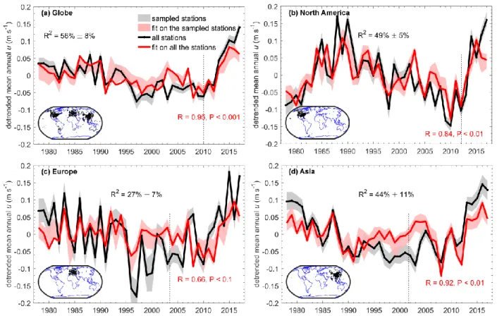
Figure 2. Factors driving the decadal variations in u. Observed (black) and reconstructed (red) 455
detrended mean annual u over the following: (a) the globe, (b) North America, (c) Europe, and (d)
456
Asia. The models are trained only using the detrended time series before the turning points. The
457
dashed line indicates the turning point (2010 for the globe, 2012 for North America, 2003 for
458
Europe, and 2001 for Asia). For the globe and each of the three continents, we select six largest
459
explanatory climate indices for the decadal variations of u with a stepwise forwarding regression
460
model. The selected climate indices are then used to reconstruct decadal variations of u via a
461
multiple regression. Uncertainties are the inter-quartile range of the results based on a randomly
462
selected 40% subset of the station pools (repeated 300 times). Inset plots indicate the locations of
463
the stations. Inset black numbers are coefficients of determination between observed and
464
reconstructed u before the turning points. Inset red numbers are correlation coefficient and its
465
significance between observed and reconstructed u after the turning points.
Figure 3. Mechanisms for the decadal variation in u. Normalized mean annual surface 467
temperature for the years with negative (a) and positive (b) anomalies of detrended wind.
468
Characteristic regions for Pacific Decadal Oscillation (PDO), North Atlantic Oscillation (NAO)
469
and Tropical Northern Atlantic Index (TNA) are outlined by green, red, and blue boxes,
470
respectively. Surface temperature over land is obtained from Climate Research Unit TEM4 with
471
a spatial resolution of 5° by 5° (ref. 50), and that over ocean is from NOAA Optimum
472
Interpolation (OI) Sea Surface Temperature V2, with a spatial resolution of 1° by 1° (ref. 51).
473
Spatial patterns of the correlation between the regional (5o × 5o) mean annual u and the following:
474
(c) TNA; (d) NAO; and (e) PDO for 1978-2017. Dotting represents significant at P < 0.05 level.
475
Decadal variations are shown in panels (f) for TNA and regional u in North America; (g) for
476
NAO and regional u in Europe; and (h) for PDO and regional u in Asia. The thin lines are annual
477
values; and the thick lines are 9-year-window moving averages. The black lines are wind speed;
478
and each of the colored lines are TNA, NAO, and PDO, respectively.
479
Figure 4. Implications of the recent reversal in global terrestrial stilling for wind energy 480
industry. (a) Frequency distribution of global average hourly u in 2010 and 2017, and the year 481
2024 assuming the same increasing rate. (b) Time series of the overall capacity factor for wind
482
generation in the U.S. (black line) and the three-order of the regional-average u (u3; blue line)
483
from 2008 to 2017. The inset scatter plot shows the significant relationship between the overall
484
capacity factor and the regional u3 (R = 0.86, P < 0.01). The inset black numbers show the trend
485
in the overall capacity factor for wind generation, and the inset red numbers show the u-induced
486
increase of capacity factor in the U.S.. (c) Mean annual u observed at a weather station near an
487
installed turbine at Deaf Smith County, the U.S. (<1 km). The inset plot shows the location. The
488
turbine was installed in 2014. The background colors separate different periods: P0, the 1980s
level when u is relative strong (1978-1995); P1, the evaluation years before the installation of the
490
turbine (2009-2013); P2, the operation years when the turbine is generating power (2014-2017).
491
(d) Mean annual wind power production at Deaf Smith County, the U.S. from different wind
492
turbines during different periods (grey: General Electric GE 1.85 – 87; green: General Electric
493
GE 2.5 – 120 turbine; blue: the theoretical maximum ratio of power that can be extracted by a
494
wind turbine given diameter of 120 m and hub height of 120 m). Error bars show the interannual
495
variability within the periods.
496 497
Figure 1. Turning point for mean global surface wind speed (u). (a) Global mean annual u 498
during 1978-2017 (black dot and line). The piecewise linear regression model indicates a
499
statistically significant turning point in 2010. The red line is the piecewise linear fit (R2 = 90%, P
500
< 0.001). The dashed line indicates the turning point. The trends before and after the turning
501
point are shown in the inset. Each grey line (n = 300) is a piecewise linear fit for a randomly
502
selected subset (40%) of the global stations. (b) Frequency distribution of the estimated turning
503
points derived from the 300 resampling results. (c) Frequency distribution of the trends in mean
504
annual u before and after the turning point from the 300 resampling results. The result is based
505
on the weather stations in the GSOD database.
Figure 2. Factors driving the decadal variations in u. Observed (black) and reconstructed (red) 507
detrended mean annual u over the following: (a) the globe, (b) North America, (c) Europe, and
508
(d) Asia. The models are trained only using the detrended time series before the turning points.
509
The dashed line indicates the turning point (2010 for the globe, 2012 for North America, 2003
510
for Europe, and 2001 for Asia). For the globe and each of the three continents, we select six
511
largest explanatory climate indices for the decadal variations of u with a stepwise forwarding
512
regression model. The selected climate indices are then used to reconstruct decadal variations of
513
u via a multiple regression. Uncertainties are the inter-quartile range of the results based on a
514
randomly selected 40% subset of the station pools (repeated 300 times). Inset plots indicate the
515
locations of the stations. Inset black numbers are coefficients of determination between observed
516
and reconstructed u before the turning points. Inset red numbers are correlation coefficient and
517
its significance between observed and reconstructed u after the turning points.
Figure 3. Mechanisms for the decadal variation in u. Normalized mean annual surface 519
temperature for the years with negative (a) and positive (b) anomalies of detrended wind.
520
Characteristic regions for Pacific Decadal Oscillation (PDO), North Atlantic Oscillation (NAO)
521
and Tropical Northern Atlantic Index (TNA) are outlined by green, red, and blue boxes,
522
respectively. Surface temperature over land is obtained from Climate Research Unit TEM4 with
a spatial resolution of 5° by 5° (ref. 50), and that over ocean is from NOAA Optimum
524
Interpolation (OI) Sea Surface Temperature V2, with a spatial resolution of 1° by 1° (ref. 51).
525
Spatial patterns of the correlation between the regional (5o × 5o) mean annual u and the following:
526
(c) TNA; (d) NAO; and (e) PDO for 1978-2017. Dotting represents significant at P < 0.05 level.
527
Decadal variations are shown in panels (f) for TNA and regional u in North America; (g) for
528
NAO and regional u in Europe; and (h) for PDO and regional u in Asia. The thin lines are annual
529
values; and the thick lines are 9-year-window moving averages. The black lines are wind speed;
530
and each of the colored lines are TNA, NAO, and PDO, respectively.
Figure 4. Implications of the recent reversal in global terrestrial stilling for wind energy 532
industry. (a) Frequency distribution of global average hourly u in 2010 and 2017, and the year 533
2024 assuming the same increasing rate. (b) Time series of the overall capacity factor for wind
534
generation in the U.S. (black line) and the three-order of the regional-average u (u3; blue line)
535
from 2008 to 2017. The inset scatter plot shows the significant relationship between the overall
536
capacity factor and the regional u3 (R = 0.86, P < 0.01). The inset black numbers show the trend
537
in the overall capacity factor for wind generation, and the inset red numbers show the u-induced
538
increase of capacity factor in the U.S.. (c) Mean annual u observed at a weather station near an
539
installed turbine at Deaf Smith County, the U.S. (<1 km). The inset plot shows the location. The
540
turbine was installed in 2014. The background colors separate different periods: P0, the 1980s
541
level when u is relative strong (1978-1995); P1, the evaluation years before the installation of the
542
turbine (2009-2013); P2, the operation years when the turbine is generating power (2014-2017).
543
(d) Mean annual wind power production at Deaf Smith County, the U.S. from different wind
turbines during different periods (grey: General Electric GE 1.85 – 87; green: General Electric
545
GE 2.5 – 120 turbine; blue: the theoretical maximum ratio of power that can be extracted by a
546
wind turbine given diameter of 120 m and hub height of 120 m). Error bars show the interannual
547
variability within the periods.