Convergence of a non-failable mean-field particle system

HAL Id: hal-01338421

https://hal.archives-ouvertes.fr/hal-01338421

HAL is a multi-disciplinary open access

archive for the deposit and dissemination of sci-entific research documents, whether they are pub-lished or not. The documents may come from teaching and research institutions in France or

L’archive ouverte pluridisciplinaire HAL, est destinée au dépôt et à la diffusion de documents scientifiques de niveau recherche, publiés ou non, émanant des établissements d’enseignement et de recherche français ou étrangers, des laboratoires

Convergence of a non-failable mean-field particle system

William Oçafrain, Denis Villemonais

To cite this version:

William Oçafrain, Denis Villemonais. Convergence of a non-failable mean-field particle system. Stochastic Analysis and Applications, Taylor & Francis: STM, Behavioural Science and Public Health Titles, 2017, 35 (4), pp.Pages 587-603. �10.1080/07362994.2017.1288136�. �hal-01338421�

Non-failable approximation method for

conditioned distributions

William Oçafrain

and Denis Villemonais

June 28, 2016

Abstract

We consider a general method for the approximation of the distribu-tion of a process condidistribu-tioned to not hit a given set. Existing methods are based on particle system that are failable, in the sense that, in many situ-ations, they are not well defined after a given random time. We present a method based on a new particle system which is always well define. More-over, we provide sufficient conditions ensuring that the particle method converges uniformly in time. We also show that this method provides an approximation method for the quasi-stationary distribution of Markov processes. Our results are illustrated by their application to a neutron transport model.

Keywords: Particle system; process with absorption; Approximation method for

degenerate processes

2010 Mathematics Subject Classification. Primary: 37A25; 60B10; 60F99.

Sec-ondary: 60J80

1 Introduction

This article is concerned with the approximation of the distribution of Markov processes conditioned to not hit a given absorbing state. Let X be a discrete

1_{École des Mines de Nancy, Campus ARTEM, CS 14234, 54042 Nancy Cedex, France}

2_{IECL, Université de Lorraine, Site de Nancy, B.P. 70239, F-54506 VandŸSuvre-lôls-Nancy}

Cedex, France

3_{Inria, TOSCA team, Villers-lès-Nancy, F-54600, France.}

time Markov process evolving in a state space E ∪ {∂}, where ∂ ∉ E is an absorb-ing state, which means that

Xn= ∂, ∀n ≥ τ∂,

whereτ_∂= min{n ≥ 0, Xn= ∂}. Our first aim is to provide an approximation

method based on an interacting particle system for the conditional distribution Pµ(Xn∈ · | n < τ∂) =Pµ

(Xn∈ · and n < τ∂)

Pµ(n < τ∂) , (1)

whereP_µ denotes the law of X with initial distributionµ on E. Our only as-sumption to achieve our aim will be that survival during a given finite time is possible from any state x ∈ E, which means that

Px(τ∂> 1) = Px(X1∈ E) > 0, ∀x ∈ E . (2)

Our second aim is to provide a general condition ensuring that the approxima-tion method is uniform in time. The main assumpapproxima-tion will be that there exist positive constants C andγ such that, for any initial distributions µ1andµ2,

°

°Pµ₁(X_n∈ · | n < τ∂) − Pµ₂(X_n∈ · | n < τ∂) ° °

T V ≤ C e−γn, ∀n ≥ 0.

This property has been extensively studied in [9]. In particular, it is known to imply the existence of a unique quasi-stationary distribution for the process X on E . Another main result of our paper is that, under mild assumptions, the approximation method can be used to estimate this quasi-stationary distribu-tion.

The naïve Monte-Carlo approach to approximate such distributions would be to consider N À 1 independent interacting particles X1, . . . , XN evolving fol-lowing the law of X underP_µand to use the following asymptotic relation

Pµ(Xn∈ · and n < τ∂) 'N →∞ 1 N N X i =1 δ_Xi n(· ∩ E) and then Pµ(Xn∈ · | n < τ∂) 'N →∞ PN i =1δXni(· ∩ E) PN i =1δXni(E ) .

However, the number of particles remaining in E typically decreases exponen-tially fast, so that, at any time n ≥ 0, the actual number of particles that are used to approximateP_µ(Xn∈ · | n < τ∂) is of order e−λnN for someλ > 0. As

a consequence, the variance of the right hand term typically grows exponen-tially fast and then the precision of the Monte-Carlo method worsens dramati-cally over time. In fact, for a finite number of particles N , the number of parti-cles X_ni belonging to E eventually vanishes in finite time with probability one. Thus the right hand term in the above equation eventually becomes undefined. Since we’re typically interested in the long time behavior of (1) or in methods that need to evolve without interruption for a long time, the naïve Monte Carlo method is definitely not well suited to fulfill our objective.

In order to overcome this difficulty, modified Monte-Carlo methods have been introduced in the recent past years by Del Moral for discrete time Markov processes (see for instance [14, 15] or the well documented web page [13], with many applications of such modified Monte-Carlo method). The main idea is to consider independent particles X1, . . . , XN evolving in E following the law of

X , but such that, at each time n ∈ N, any absorbed particle is re-introduced

to the position of one other particle, chosen uniformly among those remain-ing in E ; then the particles evolve independently from each others and so on. While this method is powerful, one drawback is that, at some random time T , all the particles will eventually be absorbed simultaneously. At this time, the in-teracting particle system is stopped and there is no natural way to reintroduce all the particles at time T + 1. When the number of particles is large and the probability of absorption is uniformly bounded away from zero, the time T is typically very large and this explain the great success of this method. However, many situations does not enter the scope of these assumptions, such as diffu-sion processes picked at discrete times or the neutron transport approximation (see Section 4). Our method is non-failable in these situations. Moreover the uniform convergence theorem provided in Section 3 also holds in these cases, under suitable assumptions.

When the underlying process is a continuous time process, one alternative to the methods of [14] has been introduced recently. The idea is to consider a continuous time N -particles system, where the particles evolve independently until one (and only one) of them is absorbed. At this time, the unique absorbed particle is re-introduced to the position of one other particle, chosen uniformly among those remaining in E . This continuous time system, introduced by Bur-dzy, Holyst, Ingermann and March (see for instance [3]), can be used to approx-imate the distribution of diffusion processes conditioned not to hit a boundary.

Unfortunately, it yields two new difficulties. The first one is that it only works if the number of jumps does not explode in finite time almost surely (which is not always the case even in non-trivial situations, see for instance [2]). The second one is that, when it is implemented numerically, one has to compute the exact absorption time of each particles, which can be cumbersome for dif-fusion processes and complicated boundaries. Note that, when this difficulties are overcome, the empirical distribution of the process is known to converge to the conditional distribution (see for instance the general result [23] and the particular cases handled in [4, 17, 20, 16, 22, 24, 1]).

Finally, it appears that both methods are not applicable in the generality we aim to achieve in the present paper and, in some cases, both method will fail (as in the case of the neutron transport example of Section 4). Let us now describe the original algorithm studied in the present paper.

Fix N ≥ 2. The particle system that we introduce is a discrete time Markov process (X_n1, . . . , X_nN)_n∈Nevolving in EN. We describe its dynamic between two successive times n and n + 1, knowing (Xn1, . . . , XnN) ∈ EN, by considering the

following random algorithm which act on any N -uplet of the form

y = ((x1, b1), . . . , (xN, bN)) ∈ (E × {0,1})N.

Algorithm 1. Initiate y by setting xi = Xni and bi = 0 for all i ∈ {1, . . . , N } and

repeat the following steps until bi= 1 for all i ∈ {1, . . . , N }.

1. Choose randomly an index i0uniformly among {i ∈ {1,..., N }, bi= 0}

2. Choose randomly a position Z ∈ E according to Px_i0(X1∈ ·). Then

• If Z = ∂, chose an index j0among {1, . . . , N }\{i0} and replace (xi0, bi0)

by (xj0, bj0) in y.

• If Z 6= ∂, replace (xi0, bi0) by (Z , 1) in y.

After a (random) finite number of iterations, the N -uplet y will satisfy bi= 1 for

all i ∈ {1,..., N }. When this is achieved, we set (X_n+11 , . . . , X_n+1N ) = (x1, . . . , xN).

Our first main result, stated in Section 2, is that, for all n ≥ 0, the empir-ical distribution of the particle system evolving following the above dynamic actually converges to the conditional distribution of the original process X at time n. We prove this result by building a continuous time Markov process

(Yt)t ∈[0,+∞[such that Ynis distributed as Xnfor all entire time n ∈ N, and such

that the general convergence result of [23] applies.

Our second main result, stated in Section 3, shows that, if the conditional distribution of the process X is exponentially mixing (in the sense of [9] or [10] for the time-inhomogeneous setting) and under a non-degeneracy condition that is usually satisfied, then the approximation method converges uniformly in time.

In Section 4, we illustrate our method by proving that it applies to neutron transport process absorbed at the boundary of an open set D.

2 Convergence of fixed time marginals

In this section, we consider the particle system defined by Algorithm 1. We state and prove our main result in a general setting.

Theorem 1. Assume that µN₀ := _N1PN

i =0δX₀i converges in law to a probability

measure µ0 on E . Then, for any n ∈ N and any bounded continuous function f : E → R, 1 N N X i =1 f (X_ni)−−−−→l aw N →∞ Eµ0( f (Xn)|n < τ∂). Moreover, E ¯ ¯ ¯ ¯ ¯ 1 N N X i =1 f (X_ni) − E_µN 0( f (Xn)|n < τ∂) ¯ ¯ ¯ ¯ ¯ ≤2(1 + p 2)kf k∞ p N E Ã 1 P_µN 0 (n < τ∂) ! (3)

We emphasize that our result applies to any process X satisfying (2), over-coming the limitations of all previously cited particle approximation methods, as illustrated by the application to a neutron transport process in Section 4.

Proof of Theorem 1. The proof is divided in two steps. First, we provide an

im-plementation of Algorithm 1 as the discrete time included chain of a contin-uous time Fleming-Viot type particle system. In particular, this step provides a mathematically tractable implementation of Algorithm 1. In a second step, we use existing results on Fleming-Viot type particle systems to deduce that the empirical distribution of the particle system converges to the conditional distribution (1).

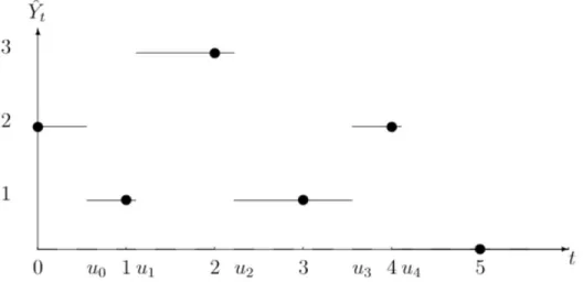
Figure 1: The points represent the values taken by the Markov chain X and the thin lines are the trajectory of Y , which jumps from Xn to Xn+1at time un. At

any time t ∈ [n,n + 1[, Bt is equal to 1 if the process has already jumped during

any interval [n, n + 1] and is equal to 0 otherwise.

Step 1 : Algorithm 1 as a Fleming-Viot type process

Let us introduce the continuous time process (Yt)t ∈[0,+∞[ defined, for any t ∈

[0, +∞[, by

Yt= X[t ]1t <u[t ]+ X[t ]+11t ≥u[t ]

where [·] denotes the integer part and (un)n∈Nis a family of independent

ran-dom variables such that, for all n ∈ N, un follows a uniform law on [n, n + 1].

With this definition, (Yt)t ≥0is a non-Markovian continuous time process such

that Ynand Xnhave the same law for all n ∈ N.

Now, we define the continuous time process (Bt)t ≥0by

Bt=

X

n∈N

1_{t ∈[u}n,n+1[, ∀t ≥ 0.

By construction, the continuous-time process (Zt)t ∈[0,+∞[defined by

Zt = (t , Yt, Bt), ∀t ∈ [0,+∞[,

is a strong Markov process evolving in F = R+× (E ∪ {∂}) × {0, 1}, with absorbing

Let us now define a Fleming-Viot type system whose particles evolve as independent copies of Z between their absorption times. More precisely, fix

N ≥ 2 and consider the following continuous time Fleming-Viot type particle

system, denoted by (Zi)_{i ∈{1,...,N }}, starting from (z1, . . . , zN) ∈ FN and evolving as

follows.

• The N particles evolve as N independent copies of Z until one of them reaches ∂F. Note that it is clear from the definition of Z that only one

particle jumps at this time.

• Then the unique killed particle is taken from the absorbing point∂F and

is instantaneously placed at the position of an other particle chosen uni-formly between the N −1 remaining ones; in this situation we say that the particle undergoes a rebirth.

• Then the particles evolve as independent copies of Z until one of them reaches∂F and so on.

For all t ∈ [0,+∞[, we denote by Ai ,Nt the number of rebirths of the it h

par-ticle occurring before time t and by AN_t the total number of rebirths before the time t . Clearly, AN_t = N X i =1 Ai ,N_t almost surely.

Also, for all t ∈ [0,+∞[, we set Zti= (t , Yti, Bti), where Yti and Bti are the marginal

component of Zi in E and {0, 1} respectively.

One can easily check that this Fleming-Viot system (considered at discrete times) is a particular implementation of the informal description of Algorithm 1 in the introduction. Indeed, at any time n ≥ 0, the Fleming-Viot system is de-fined so that

(Y_ni, B_ni) = (Yni, 0).

Then, at each time t ∈ [n,n+1[, the index of the next moving particle i ∈ {1,...,n} belongs to the set of particles j ∈ {1,..., N } such that Bnj = 0. Moreover,

condi-tionally to B_tj = 0, the jumping times of these particles are independent and identically distributed (uniformly on [t , n + 1[). As a consequence i is chosen uniformly among these indexes (this is the first step of Algorithm 1). Then, at the jumping timeτ, the position Y_τi of the particle i is chosen according to

P_Yi

t(X1∈ ·) and B

i

τis set to 1. If the position at timeτ is ∂, then the particle i

un-dergoes a rebirth and hence (Y_τi, B_τi) is replaced by (Y_τk, B_τk) = (Ytk, Btk), where k

is chosen uniformly among {1, . . . , N }\{i }. Hence the second step of Algorithm 1 is completed. Finally, the procedure is repeated until all the marginals Bi are equal to 1, as in Algorithm 1.

In particular, for any n ≥ 0, the random variable (Xn1, . . . , XnN) obtained from

Algorithm 1 and the variable (Y_n1, . . . , Y_nN) obtained from the Fleming-Viot type algorithm have the same law.

Step 2 : Convergence of the empirical system.

In this step, we consider a sequence of initial positions (Y₀1, . . . , Y_NN)_{N ≥2}such that _N1PN

i =0δY₀i converges in law to a probability measureµ0on E . Our aim is

to prove that, for any n ∈ N and any bounded continuous function f : E → R, 1 N N X i =1 f (Y_ni)−−−−→l aw N →∞ Eµ0( f (Yn)|n < τ∂).

Note that, since Xn and Yn share the same law, this immediately implies the

first part of Theorem 1.

Since (Z1, . . . , ZN) is a Fleming-Viot type process without simultaneous killings, [23, Theorem 2.2] implies that it is sufficient to prove that, for all N ≥ 2 and al-most surely,

AN_t < ∞, ∀t ≥ 0, (4)

where we recall that AN_t is number of rebirths undergone by the Fleming-Viot type system with N particles before time t .

First, let us remark that P(AN t = ∞) É P(A[t ]+1N = ∞). Moreover, P(AN [t ]+1= ∞) = P Ã [t ] [ i =0 {A_{i +1}N − AN_i = ∞} ! É [t ] X i =0 P¡AN i +1− A N i = ∞¢ .

Using the weak Markov property at time i , it is sufficient to prove that P(AN

for any initial distribution of the Fleming-Viot type process (Y1, . . . , YN) in order to conclude that P¡AN i +1− A N i = ∞¢ = 0, ∀i ≥ 0.

and hence that (4) holds true.

But AN₁ = ∞ if and only if there exists at least one particle for which there is an infinity of rebirths, hence

P(AN t = ∞) É N X i =1 P³Ai ,N₁ = ∞ ´ (6) Now, when a particle undergoes a rebirth, it jumps on the position of one of the N − 1 remaining particles. As a consequence, at any time t ∈ [0,1[, the po-sition Y_ti of the particles i ∈ {1,..., N } such that Bit = 0 are included in the set

{Y₀1, . . . , Y₀N}. In particular, the probability that such a particle undergoes a re-birth during its next move is bounded above by

c := max

i ∈{1,...,N }PY0i(X1= ∂) < 1.

Hence, a classical renewal argument shows that the probability that a particle undergoes n rebirths is bounded above by cn. This implies that the probability that a particle undergoes an infinity of rebirths is zero. This, together with (6) implies (5), which concludes the proof of the first part of Theorem 1.

In order to conclude the proof, let us simply remark that, for a determin-istic value ofµN₀, the inequality of Theorem 1 is directly provided by [23, The-orem 2.2]. Now, ifµN₀ is a random measure, the inequality is obtained by in-tegrating the deterministic case inequality with respect to the law ofµ₀N. This concludes the proof of Theorem 1.

3 Uniform convergence for uniformly mixing

con-ditioned semi-groups

In a recent paper [9], necessary and sufficient conditions on an absorbed Markov process X were obtained to ensure that a process satisfies

°

°Pµ₁(X_n∈ · | n < τ∂) − Pµ₂(X_n∈ · | n < τ∂) ° °

whereγ and C are positive constants. In particular this implies the existence of a unique quasi-stationary distributionνQSD for X , that is a unique probability

measure on E such thatP_νQSD(Xn∈ · | n < τ∂) = νQSD, for all n ≥ 0. General and classical results on quasi-stationary distributions (see for instance [18, 21, 11]) implies that there existsλ0> 0 such that

PνQSD(n < τ∂) = e−λ

0n

, ∀n ≥ 0. (8)

The exponential convergence property 7 holds for a large class of processes, including birth and death processes with catastrophe, branching Brownian par-ticles, neutron transport approximations processes (see [9]), one dimensional diffusion with or without killing (see [8, 6]), multi-dimensional birth and death processes (see [7]) and multi-dimensional diffusion processes (see [5]). Also, similar properties can be proved for time-inhomogeneous processes, as stressed in the recent paper [10], with applications to time-inhomogeneous diffusion processes and birth and death processes in a quenched random environment.

In this section, we state and prove our second main result, which states that, if (7) holds and if, for any n0≥ 1, there exists ε0> 0 such that

inf

x∈EPx(PX1(n0< τ∂) ≥ ε0| 1 < τ∂) = c0> 0, (9)

then the convergence of the empirical distribution of the particle system de-scribed in Algorithm 1 converges uniformly in time to the conditional distribu-tion of the process X .

We emphasize that the additional assumption (9) is true for many processes satisfying (7), for instance in the case of one-dimensional diffusion processes, multidimensional diffusion processes or piecewise deterministic Markov pro-cesses (this the detailed examples of Section 4). As far as we know, none of this processes were covered in this generality by previous methods. In particular, this is the first method that allows the approximation of the conditional distri-bution of the neutron transport approximation process (see Section 4), since in this case it easy to check that, with probability one, all the particles will even-tually hit the boundary at the same time when using previous algorithms. The methods also allows to handle the case of the diffusion process on E = (0,2] killed at 0, reflected at 2 and solution to the following stochastic differential equation

d Xt = dWt+

1

In this case, the continuous time Fleming-Viot approximation method intro-duced in [3] explodes in finite time almost surely, as proved in [2]. As a matter of fact, it is not known if the Fleming-Viot type particle system is well defined as soon as the diffusion coefficient is degenerated or not regular toward the boundary 0. On the contrary, our assumption holds true for fairly general one dimensional diffusion processes, thanks to the study provided in [8]. Hence our approximation method is valid and, using the next results, converges uni-formly in time for both neutron transport processes and degenerate diffusion processes.

For any n ∈ N, we define the empirical distribution of the process at time n asµ_nN=_N1

N

P

i =1δX

i

n, and for any bounded measurable function f on E , we set

µN n( f ) = 1 N N X i =1 f (X_ni).

Theorem 2. Assume that (7) and (9) holds true. Then there exist two constants

C > 0 and α < 0, such that, for all δ > 0 and all measurable function f : E → R bounded by 1, E³¯¯ ¯µ N n( f ) − EµN 0( f (Xn) | n < τ∂) ¯ ¯ ¯ ´ ≤C N α δ +C P ³ P_µN 0(n0< τ∂) ≤ ε0δ ´ , ∀n ≥ 0, with α = −γ 2¡ λ0+ γ ¢ < 0.

In the case where the initial position of the particle system are drawn as in-dependent random variables distributed following the same lawµ, then, choos-ingδ > 0 small enough so that P_µ(n0< τ∂) ≥ 2ε0δ, basic concentration

inequal-ities and the equalityE(P_Xi

0(n0< τ∂)) = Pµ(n0< τ∂) imply that P³P_µN 0(n0< τ∂) ≤ ε0δ ´ ≤ P Ã Pµ(n0< τ∂) − 1 N N X i =1 P_Xi 0(n0< τ∂) ≥ ε0δ ! ≤ e−N β,

Corollary 1. Assume that (X₀1, . . . , X₀N) are independent and identically distributed

following a given law µ on E. If (7) and (9) hold true, then there exist two constants C_µ> 0 and α < 0 such that, and all measurable function f : E → R

bounded by 1, E³¯¯ ¯µ N n( f ) − EµN 0( f (Xn) | n < τ∂) ¯ ¯ ¯ ´ ≤ CµNα, ∀n ≥ 0,

whereα is the same constant as in Theorem 2.

We emphasize that the above results and their proofs can be adapted to the time-inhomogeneous setting of [10], with appropriate modifications of As-sumption (9).

The following result is specific to the time-homogeneous setting and is proved at the end of this section.

Theorem 3. Under the assumptions of Theorem 2, the particle system (X1, . . . , XN)

is exponentially ergodic, which means that it admits a stationary distribution MN (which is a probability measure on EN) and that there exists positive con-stants CN andγN such that

° °MN− Law(X_n1, . . . , X_nN) ° ° T V ≤ CNe−γ Nt_.

Moreover, there exists a positive constant C > 0 such that, for all measurable function f : E → R bounded by 1, EMN ¡¯ ¯µN₀( f ) − ν_QSD( f ) ¯ ¯¢ ≤ C Nα, (10)

where α is the same as in Theorem 2 and (X₀1, . . . , X₀N) is distributed following

MN.

Proof of Theorem 2. Using the exponential convergence assumption (7), we

de-duce that, for any function f : E → R such that kf k∞= 1 and all n ≥ n1≥ 0,

E³¯¯ ¯µ N n( f ) − EµN 0( f (Xn) | n < τ∂) ¯ ¯ ¯ ´ ≤ E ³¯ ¯ ¯µ N n( f ) − EµN n−n1( f (Xn) | n < τ∂) ¯ ¯ ¯ ´ + E ³¯ ¯ ¯EµN_n−n1( f (Xn) | n < τ∂) − EµN₀( f (Xn) | n < τ∂) ¯ ¯ ¯ ´ ≤ E ³¯ ¯ ¯µ N n( f ) − EµN n−n1( f (Xn) | n < τ∂) ¯ ¯ ¯ ´ +C e−γn1_. (11)

Denoting by (Fn)n∈Nthe natural filtration of the particle system (Xn1, . . . , XnN)n∈N,

we deduce from Theorem 1 that, almost surely, E³¯¯ ¯µ N n( f ) − E_µN n−n1( f (Xn) | n < τ∂) ¯ ¯ ¯ | Fn−n1 ´ ≤ 2 ∧ 2(1 + p 2) P_µN n−n1(n1< τ∂) p N.

Hence, for allε > 0, E³¯¯ ¯µ N n( f ) − E_µN n−n1( f (Xn) | n < τ∂) ¯ ¯ ¯ ´ ≤ 2P ³ P_µN n−n1(n1< τ∂) ≤ ε ´ +2(1 + p 2) εpN P ³ P_µN n−n1(n1< τ∂) > ε ´ . But [9, Theorem 2.1] entails the existence of a measure ν on E and positive constants c1, n0> 0 and c2> 0 such that for any n ∈ N and x ∈ E,

½

Px(Xn0∈ · | n0< τ∂) ≥ c1ν(·)

Pν(n < τ∂) ≥ c2Px(n < τ∂)

Note that, from now on, n0is a fixed constant. This entails

Pµ(n1< τ∂) ≥ Pµ(n0< τ∂)c1Pν(n1− n0< τ∂)

≥ Pµ(n0< τ∂)c1c2max

x∈E Px(n1− n0< τ∂)

≥ c1c2Pµ(n0< τ∂)e−λ0(n1−n0),

whereλ0> 0 is the constant of (8). We deduce that

E³¯¯ ¯µ N n( f ) − EµN n−n1( f (Xn) | n < τ∂) ¯ ¯ ¯ ´ ≤ 2P ³ P_µN n−n1(n0< τ∂) ≤ c3εe (n1−n0)λ0´ +2(1 + p 2) εpN . (12)

with c3=_c11_c2. Our aim is now to controlP

³ P_µN

n(n0< τ∂) ≤ ε ´

, uniformly in n ≥ 0 and for allε ∈ (0,ε0/2). In order to do so, we make use of the following lemma,

proved at the end of this subsection.

Lemma 1. There exists p0> 0 and δ > 0 such that, for any value of µ₀N,

P¡µN

1(P·(n0< τ∂)) ≤ δε0¢ ≤ 1 − p0. Moreover, ifP_µN

0(1 < τ∂) > ε for some ε ∈ (0,c0ε0), then

P¡µN 1(P·(n0< τ∂)) ≤ ε¢ ≤ 2(1 + p 2) ε(c0ε0− ε) p N.

From this lemma (where we assume without loss of generality thatδ ≤ 1/2), from the Markov property applied to the particle system and since P_µN

0(n0< τ∂) > ε implies PµN

0(1 < τ∂) > ε, we deduce that, for any ε ∈ (0,δε0),

P³P_µN n+1(n0< τ∂) ≤ ε ´ ≤ 2(1 + p 2) ε(ε0/2 − ε) p NP ³ P_µN n(n0< τ∂) > ε ´ + (1 − p0)P ³ P_µN n(n0< τ∂) ≤ ε ´ ≤ 2(1 + p 2) ε(ε0/2 − ε) p N + (1 − p0)P ³ P_µN n(n0< τ∂) ≤ ε ´ ≤ 2(1 + p 2) p0ε(ε0/2 − ε) p N + (1 − p0) n+1_P³_P µN 0(n0< τ∂) ≤ ε ´ , (13) where the last line is obtained by iteration over n.

This and equation (12) imply that, for anyε ∈ ¡0,ε0δ/(c3e(n1−n0)λ0)¢,

E³¯¯ ¯µ N n( f ) − EµN n−n1( f (Xn) | n < τ∂) ¯ ¯ ¯ ´ ≤ 4(1 + p 2) p0c3εe(n1−n0)λ0(ε0/2 − c3εe(n1−n0)λ0) p N + 2(1 +p2)(1 − p0)n−n1P ³ P_µN 0(n0< τ∂) ≤ c3εe (n1−n0)λ0´ +2(1 + p 2) εpN .

Takingε = ε0δ/(c3e(n1−n0)λ0) and assuming, without loss of generality, thatδ ≤

1/4, we obtain E³¯¯ ¯µ N n( f ) − EµN n−n1( f (Xn) | n < τ∂) ¯ ¯ ¯ ´ ≤16(1 + p 2) p0ε2₀δ p N + 2(1 +p2)(1 − p0)n−n1P ³ P_µN 0(n0< τ∂) ≤ ε0δ ´ +2(1 + p 2)c2en1λ0 ε0δ p N .

Finally, using inequality (11) and taking

n1= ¹ ln N 2¡λ0+ γ ¢ º ,

straightforward computations implies the existence of a constant C > 0 such that, for all n ≥ n1,

E³¯¯ ¯µ N n( f ) − EµN 0( f (Xn) | n < τ∂) ¯ ¯ ¯ ´ ≤C N α δ +C P ³ P_µN 0(n0< τ∂) ≤ ε0δ ´

with

α = −γ

2¡λ0+ γ

¢ < 0. Now, for n ≤ n1, we have

E³¯¯ ¯µ N n( f ) − EµN 0( f (Xn) | n < τ∂) ¯ ¯ ¯ ´ ≤ E  2 ∧ 2(1 +p2) P_µN 0 (n1< τ∂) p N   ≤ E  2 ∧ 2(1 +p2)en1λ0 c3P_µN 0 (n0< τ∂) p N   ≤ 2P ³ P_µN 0(n0< τ∂) ≤ ε0δ ´ +2(1 + p 2)en1λ0 ε0δ p N .

Using the same computations as above, this concludes the proof of Theorem 2.

Proof of Lemma 1. Assume that P_µN

0(1 < τ∂) > ε. We obtain from Theorem 1

that E³¯¯ ¯µ N 1(P·(n0< τ∂)) − EµN 0 ¡ PX1(n0< τ∂) | 1 < τ∂ ¢¯_¯ ¯ ´ ≤2(1 + p 2)kP·(n0< τ∂)k∞ εpN .

Markov’s inequality thus implies that, for allδ > 0, P³¯¯ ¯µ N 1(P·(n0< τ∂)) − E_µN 0 ¡ PX1(n0< τ∂) | 1 < τ∂ ¢¯ ¯ ¯ ≥ δ ´ ≤2(1 + p 2) εδpN

and hence that P³µN 1(P·(n0< τ∂)) ≤ EµN 0 ¡ PX1(n0< τ∂) | 1 < τ∂¢ − δ ´ ≤2(1 + p 2) εδpN .

But, by Assumption (9), we have P_µN

0 ¡ PX1(n0< τ∂) ≥ ε0| 1 < τ∂¢ ≥ c0, so that E_µN 0 ¡ PX1(n0< τ∂) | 1 < τ∂¢ ≥ c0ε0. We deduce that P¡µN 1(P·(n0< τ∂)) ≤ ε0c0− δ¢ ≤ 2(1 + p 2) εδpN .

Choosingδ = c0ε0− ε, we finally obtained P¡µN 1(P·(n0< τ∂)) ≤ ε¢ ≤ 2(1 + p 2) ε(c0ε0− ε) p N.

In the general case (when one does not have a good control onP_µN

0(1 < τ∂)),

the above strategy is bound to fail since we do not have a good control on the distance between the conditioned semi-group and the empirical distribution of the particle system. As a consequence, we need to take a closer look at Al-gorithm 1. As explained in the description of this alAl-gorithm, the position of the system at time 1 is computed from the position of the system at time 0 through several steps, each step being composed of two stages. We denote by ¯k the

number of steps needed to compute the position of the system at time 1. For any step k ≥ 1, we denote by X₀i ,k the position of the it h particle at the beginning of step k, by b_ikthe state of the it hparticle at the beginning of step k, and by ik∈ {i ∈ {1, . . . , N }, b_ik= 0} the index of the particle chosen during the first

stage of step k. With this notation, the process ³

(X₀i ,k∧ ¯k, bk∧ ¯k_i )_{i ∈{1,...,N }}, i_{k∧ ¯k} ´

k∈N

is a Markov chain. In what follows, we denote by (Gk)k≥1 the natural filtration

of this Markov chain.

We also introduce the quantities

Nk= ]{i ∈ {1, . . . , N }, bk_i = 1 (at the beginning of the kt hstep)},

N_k0 = ]{i ∈ {1, . . . , N }, bk_i = 1 and P_Xi ,k

0 (n0< τ∂) ≥ ε0}, N_k00= ]{i ∈ {1, . . . , N }, bk_i = 1 and P_Xi ,k

0 (n0< τ∂) < ε0}.

Of course, we have Nk= N_k0+ N_k00and, at the beginning of the first step, one has

N1= N₁0= N₁00= 0. For any k ≥ 1, conditionally to Gkand on the event k ≤ ¯k, the

position of Xik,k+1

0 is chosen with respect to

P X₀ik ,k(X1∈ ·) + PX₀ik ,k(τ∂≤ 1) 1 N − 1 N X i =1,i 6=ik δ_Xi ,k.

Hence, conditionally toGkand on the event k ≤ ¯k, (N_k+10 , N_k+100 ) is equal to            (N_k0, N_k00) with prob.P X₀ik ,k(τ∂≤ 1) N −1−Nk N −1 , (N_k0+ 1, N_k00) with prob.P X₀ik ,k ¡ PX1(n0< τ∂) ≥ ε0¢ + P_Xik ,k 0 (τ_∂≤ 1) N 0 k N −1, (N_k0, N_k00+ 1) with prob. P X₀ik ,k¡0 < PX1(n0< τ∂) < ε0¢ + P_Xik ,k 0 (τ_∂≤ 1) N 00 k N −1. (14) From Assumption (9), we deduce that, conditionally to Gk and on the event

k ≤ ¯k, (N_k+10 , N00 k+1) is equal to            (N_k0, N_k00) with prob.P X₀ik ,k(τ∂≤ 1) N −1−Nk N −1 , (N_k0+ 1, N_k00) with prob. ≥ c0P_Xik ,k 0 (1 < τ∂) + P_Xik ,k 0 (τ_∂≤ 1) N 0 k N −1, (N_k0, N_k00+ 1) with prob. ≤ (1 − c0)P X₀ik ,k(1 < τ∂) + PX₀ik ,k(τ∂≤ 1) N00 k N −1. (15)

Let us denote by k1, . . . , kn, . . . the successive step numbers during which the

sequence (Nk)k≥1jumps, that is

k1= inf{k ≥ 1, Nk+16= Nk},

k_n+1= inf{k ≥ kn+ 1, Nk+16= Nk}, ∀n ≥ 1.

It is clear that, for all n ≥ 1, kn+ 1 is a stopping time with respect to the

filtra-tionG . We are interested in the sequence of random variables (Un)n≥1, defined

by

Un= N_k0_n+1, ∀n ∈ {1,..., N }.

Conditionally toGkn+1 (the filtration (Gk)k≥1before the stopping time kn+ 1), we deduce from (14) that, for all x ∈ E,

P(Un+1= Un+ 1 | Gkn+1, X i_kn+1,k_n+1 0 = x) ≥ Px(1 < τ∂)c0+ Px(τ∂≤ 1) N0 kn +1 N −1 Px(1 < τ∂) + Px(τ∂≤ 1) N_{kn +1} N −1 ≥ c0∧ N_k0 n+1 N_kn+1 = c0∧ Un n ,

since Nkn+1= n almost surely. We deduce that P(Un+1= Un+ 1 | U1, . . . ,Un) ≥ c0∧ Un n P(Un+1= Un| U1, . . . ,Un) = 1 − P(Un+1= Un+ 1 | U1, . . . ,Un) ≤ 1 − c0∧ Un n .

Moreover, Assumption (9) entails thatP(U1= 1) ≥ c0> 0.

As a consequence, there exists a coupling between (Un)n∈Nand the Markov

chain (Vn)n≥1with initial lawP(V1= 1) = c0and transition probabilities

P(Vn+1= Vn+ 1 | V1, . . . ,Vn) = c0∧ Vn

n ,

P(Vn+1= Vn| V1, . . . ,Vn) = 1 − P(Vn+1= Vn+ 1 | V1, . . . ,Vn)

such that Un ≥ Vn, for all n ∈ {1,..., N }. The process (Vn/n)n∈N is a positive

super-martingale (and a martingale if c0= 1) and hence it converges to a

ran-dom variable R_∞almost surely as n → ∞. Let us now prove that R∞is not equal

to zero almost surely.

Consider a Pólya urn starting with n0 balls with one white one, that is a

Markov chain (Wn)n∈NinN such that W0= 1 and

P(Wn+1= Wn+ 1 | Wn) = Wn n + n0 , ∀n ≥ 0, P(Wn+1= Wn| Wn) = 1 − Wn n + n0, ∀n ≥ 0.

It is well known that (Wn/n)n∈N is a positive and bounded martingale which

converges almost surely to a random variable S_∞distributed following a Beta distribution with parameters (1, n0−1). In particular, this implies that the event

{Wk/k ≤ c0, ∀k ≥ 0} has a positive probability and that, conditionally to this

event, Wn/n converges to a positive random variable :

1Wk/k≤c0, ∀k≥0 Wn n a.s. −−−−→ n→∞ 1Wk/k≤c0, ∀k≥0S∞.

Since (V_n+n0)_n∈Nand (Wn)n∈Nhave the same transition probabilities at time n

from states u ∈ N such that u/n ≤ c0, there exists a coupling such that

and hence such that

1V0≥1R∞≥ 1V0≥11Wk/k≤c0, ∀k≥0S∞almost surely.

Since the right hand side is positive with positive probability, we deduce that

R_∞is positive with positive probability. But R_∞> 0 implies that infn≥0Vn/n > 0,

thus there existsδ > 0 such that P µ inf n≥0 Vn n > δ ¶ > 0.

Because of the relation between Vnand Un, we deduce that

p0:= P Ã N0 kN N > δ ! = P µ UN N > δ ¶ > 0. By definition of N_k0 N, N0 kN N > δ implies µ N 1(P·(n0< τ∂)) > δε0and hence P¡µN 1(P·(n0< τ∂)) ≤ δε0¢ ≤ 1 − p0.

This concludes the proof of Lemma 1.

Proof of Theorem 3. We first prove the exponential ergodicity of the particle

sys-tem and then deduce (10).

Using Lemma 1, we know that, for any initial distribution of (X₀1, . . . , X₀N), P(P_µN

1(n0< τ∂) > δε0) ≥ p0.

On the event P_µN

1(n0< τ∂) > δε0, there exists at least one particle satisfying

P_Xi

1(n0< τ∂) > δε0. Let us denote by I ⊂ {1,..., N } the set of indexes of such

par-ticles and by J = {1,..., N } \ I the set of indexes j such that P_Xj

1

(n0< τ∂) ≤ δε0.

The probability that the]J first steps of Algorithm 1 concern the indexes of]J in strictly increasing order is strictly lowered by 1/N]J and hence by 1/NN. For each of this step, the probability that the chosen particle with index in J is killed and then is sent to the position of a particle with index in I is lowered by (1 − δε0)]I/N and hence by (1 − δε0)/N . Overall, the probability that, after the

particle with index in I is bounded below by 1/NN× (1 − δε0)]J/N]J and hence

by (1 − δε0)N/N2N.

On this event, the probability that, for each next step in the algorithm up to time n0+ 1, the chosen particle jumps without being absorbed is bounded

below by (δε0)N. But, using [9, Theorem 2.1], we know that, under

Assump-tion 7, there exist a probability measureν on E and a constant c1> 0 such that

Px(Xn0∈ · | n0< τ∂) ≥ c1ν(·). Since the particles are independent on the event

where none of them is killed, we finally deduce that the distribution of the par-ticle system at time n0+ 1 satisfies

P¡(X1 n0+1, . . . , X 1 n0+1) ∈ ·¢ ≥ p0(δε N 0(1 − δε0)N/N2Nc1Nν⊗N(·).

Classical coupling criteria (see for instance [19]) entails the exponential ergod-icity of the particle system.

Let us now prove that (10) holds. Consider x ∈ E and δ > 0 such that Px(n0< τ∂) > ε0δ. Then, applying Theorem 2 to the particle system with initial position

(X₀1, . . . , X₀N) = (x,..., x), we deduce that, for all n ≥ 0, E¡¯¯µN

n( f ) − Ex( f (Xn) | n < τ∂)¯¯¢ ≤

C Nα δ .

Using the exponential ergodicity of the particle system and the exponential convergence (7), we deduce that

EMN ¡¯ ¯µN₀( f ) − ν_QSD( f ) ¯ ¯¢ ≤ C Nα δ + 2CNe−γN n +C e−γn.

Letting n tend toward infinity implies (10) and concludes the proof of Theo-rem 3.

4 Example: Absorbed neutron transport process

The propagation of neutrons in fissible media is typically modeled by neutron transport systems, where the trajectory of the particle is composed of straight exponential paths between random changes of directions [12, 25]. The behav-ior of a neutron before its absorption by a medium is related to the behavbehav-ior of neutron tranport before extinction, where extinction corresponds to the exit of a neutron from a bounded set D.

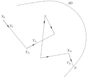
We recall the setting of the neutron transport process studied in [9]. Let D be an open connected bounded domain ofR2, let S2be the unit sphere ofR2 andσ(du) be the uniform probability measure on S2. We consider the Markov process (Xt,Vt)t ≥0 in D × S2constructed as follows: Xt =

Rt

0Vsd s and the

ve-locity Vt ∈ S2 is a pure jump Markov process, with constant jump rate λ > 0

and uniform jump probability distributionσ. In other words, Vt jumps to i.i.d.

uniform values in S2 at the jump times of a Poisson process. At the first time where Xt 6∈ D, the process immediately jumps to the cemetery point ∂,

mean-ing that the process is absorbed at the boundary of D. An example of path of the process (X ,V ) is shown in Fig. 2. For all x ∈ D and u ∈ S2, we denote byPx,u

(resp.Ex,u) the distribution of (X ,V ) conditionned on (X0,V0) = (x,u) (resp. the

expectation with respect toPx,u).

Figure 2: A sample path of the neutron transport process (X ,V ). The times

J1< J2< . . . are the successive jump times of V .

We also assume the following condition on the boundary of the bounded open set D. This is an interior cone type condition satisfied for example by convex open sets ofR2and by open sets with C2boundaries.

Assumption (H) on D. We assume that there existsε > 0 such that

• there exists 0 < sε< tε andσ > 0 such that, for all x ∈ D \ Dε, there exists

Kx⊂ S2measurable such thatσ(Kx) ≥ σ and for all u ∈ Kx, x + su ∈ Dεfor

all s ∈ [sε, tε] and x + su 6∈ ∂D for all s ∈ [0, sε].

The next proposition implies that the approximation method introduced in this paper converges uniformly in time toward the conditional distribution of (X ,V ).

Proposition 1. The absorbed Markov process (X ,V ) satisfies the assumptions of

Theorem 2.

Proof of Proposition 1. Theorem 4.3 from [9] states that the Markov process (X ,V )

satisfies the exponential convergence condition (7). It only remains to check that that Assumption (9) is also satisfied.

By [9, (4.3)], for any n0≥ 1, there exists a constant cn0> 0 such that cn0:= inf

(x,u)∈Dε×S2P(x,u)(1 + n0< τ∂) > 0. (16)

In particular, we deduce that, for all n0≥ 0,

P(x,u)(P(X1,V1)(n0< τ∂) | 1 < τ∂) ≥ cn0, ∀(x, u) ∈ Dε× S

2_{. (17)}

Now, fix (x, u) ∉ Dε× S2and consider the first (deterministic) time s(x, u) when the ray starting from x with direction u hits D_εor∂D, defined by

s(x, u) = inf{t ≥ 0, such that x + tu ∈ Dε∪ ∂D}.

Let us first assume that x + s(x,u)u ∈ ∂Dε. Then x + (s(x,u) + η)u ∈ Dεfor some

η > 0 and hence

P(x,u)(Xs(x,u)+η∈ Dε) ≥ P¡ J1> s(x, u) + η¢ = e−(s(x,u)+η)≥ e−diam(D),

where J1< J2< · · · denotes the successive jump times of the process V . Using

the Markov property, we deduce from (16) that

P(x,u)(1 + n0< τ∂) ≥ P(s + η + 1 + n0< τ∂) ≥ e−diam(D)cn0. (18)

This implies that, for all n0≥ 1 and all (x, u) ∉ Dε× S2such that x + s(x,u)u ∈ ∂Dε,

Let us now assume that x + s(x,u)u ∈ ∂D. Using Assumption (H), we obtain P(x,u)(∃t ∈ [0, s) s.t. Xt+ s(Xt,Vt)Vt∈ ∂Dε) ≥ P(x,u)(J1< s, VJ1∈ Kx+u J1, J2> s)

≥ (1 − e−s)σe−s. Using the strong Markov property and (18), we deduce that

P(x,u)(1 + n0< τ∂) ≥ (1 − e−s)σe−se−diam(D)cn0≥ (1 − e

−s∧1_)σe−2diam(D)_c

n0.

If s ≤ 1, then 1 < τ∂ implies that the process jumps at least one time before

reaching∂D, that is before time s, so that P(x,u)(1 < τ∂) ≤ P(J1≤ s) = 1 − e−s.

Using the Markov property, we deduce that, for s ≤ 1 or s > 1,

P(x,u)(P(X1,V1)(n0< τ∂) | 1 < τ∂) = P(x,u)(1 + n0< τ∂| 1 < τ∂)

≥ (1 − e−1)σe−2diam(D)cn0.

This, Equations (17) and (19) together imply that Assumption (9) is fulfilled for all (x, u) ∈ D,S2. This concludes the prood of Proposition 1.

References

[1] A. Asselah, P. A. Ferrari, P. Groisman, and M. Jonckheere. Fleming-Viot se-lects the minimal quasi-stationary distribution: The Galton-Watson case.

Ann. Inst. H. Poincaré Probab. Statist., 52(2):647–668, 05 2016.

[2] M. Bieniek, K. Burdzy, and S. Pal. Extinction of fleming-viot-type particle systems with strong drift. Electron. J. Probab., 17:no. 11, 1–15, 2012. [3] K. Burdzy, R. Holyst, D. Ingerman, and P. March. Configurational transition

in a fleming-viot-type model and probabilistic interpretation of laplacian eigenfunctions. J. Phys. A, 29(29):2633–2642, 1996.

[4] K. Burdzy, R. Hołyst, and P. March. A Fleming-Viot particle representation of the Dirichlet Laplacian. Comm. Math. Phys., 214(3):679–703, 2000. [5] N. Champagnat, A. Coulibaly-Pasquier, and D. Villemonais. Exponential

convergence to quasi-stationary distribution for multi-dimensional diffu-sion processes. ArXiv e-prints, Mar. 2016.

[6] N. Champagnat and D. Villemonais. Exponential convergence to quasi-stationary distribution for absorbed one-dimensional diffusions with killing. ArXiv e-prints, Oct. 2015.

[7] N. Champagnat and D. Villemonais. Quasi-stationary distribution for multi-dimensional birth and death processes conditioned to survival of all coordinates. ArXiv e-prints, Aug. 2015.

[8] N. Champagnat and D. Villemonais. Uniform convergence of conditional distributions for absorbed one-dimensional diffusions. ArXiv e-prints, June 2015.

[9] N. Champagnat and D. Villemonais. Exponential convergence to quasi-stationary distribution and Q-process. Probab. Theory Related Fields,

164(1-2):243–283, 2016.

[10] N. Champagnat and D. Villemonais. Uniform convergence of penalized time-inhomogeneous Markov processes. ArXiv e-prints, Mar. 2016. [11] P. Collet, S. Martínez, and J. San Martín. Quasi-stationary distributions.

Probability and its Applications (New York). Springer, Heidelberg, 2013. Markov chains, diffusions and dynamical systems.

[12] R. Dautray and J.-L. Lions. Mathematical analysis and numerical methods

for science and technology. Vol. 6. Springer-Verlag, Berlin, 1993.

[13] P. Del Moral. Feynman-Kac models and interacting particle systems.

http://web.maths.unsw.edu.au/~peterdel-moral/simulinks. html.

[14] P. Del Moral. Measure-valued processes and interacting particle systems. Application to nonlinear filtering problems. Ann. Appl. Probab., 8(2):438– 495, 1998.

[15] P. Del Moral and L. Miclo. Particle approximations of Lyapunov expo-nents connected to Schrödinger operators and Feynman-Kac semigroups.

ESAIM Probab. Stat., 7:171–208, 2003.

[16] P. A. Ferrari and N. Mari´c. Quasi stationary distributions and Fleming-Viot processes in countable spaces. Electron. J. Probab., 12:no. 24, 684–702 (electronic), 2007.

[17] I. Grigorescu and M. Kang. Hydrodynamic limit for a Fleming-Viot type system. Stochastic Process. Appl., 110(1):111–143, 2004.

[18] S. Méléard and D. Villemonais. Quasi-stationary distributions and popu-lation processes. Probab. Surv., 9:340–410, 2012.

[19] S. Meyn and R. Tweedie. Markov chains and stochastic stability. Cam-bridge University Press New York, NY, USA, 2009.

[20] M. Rousset. On the control of an interacting particle estimation of Schrödinger ground states. SIAM J. Math. Anal., 38(3):824–844

(elec-tronic), 2006.

[21] E. A. van Doorn and P. K. Pollett. Quasi-stationary distributions for discrete-state models. European J. Oper. Res., 230(1):1–14, 2013.

[22] D. Villemonais. Interacting Particle Systems and Yaglom Limit Approxi-mation of Diffusions with Unbounded Drift. Electron. J. Probab., 16:no. 61, 1663–1692, 2011.

[23] D. Villemonais. General approximation method for the distribution of markov processes conditioned not to be killed. ESAIM: Probability and

Statistics, eFirst, 2 2014.

[24] D. Villemonais. Minimal quasi-stationary distribution approximation for a birth and death process. Electron. J. Probab., 20:no. 30, 1–18, 2015. [25] A. Zoia, E. Dumonteil, and A. Mazzolo. Collision densities and mean

resi-dence times for d -dimensional exponential flights. Phys. Rev. E, 83:041137, Apr 2011.