HAL Id: hal-02154980
https://hal.archives-ouvertes.fr/hal-02154980
Submitted on 18 Dec 2019
HAL is a multi-disciplinary open access
archive for the deposit and dissemination of
sci-entific research documents, whether they are
pub-lished or not. The documents may come from
teaching and research institutions in France or
abroad, or from public or private research centers.
L’archive ouverte pluridisciplinaire HAL, est
destinée au dépôt et à la diffusion de documents
scientifiques de niveau recherche, publiés ou non,
émanant des établissements d’enseignement et de
recherche français ou étrangers, des laboratoires
publics ou privés.
Constructing Minimal Phylogenetic Networks from
Softwired Clusters is Fixed Parameter Tractable
Steven Kelk, Celine Scornavacca
To cite this version:
Steven Kelk, Celine Scornavacca.
Constructing Minimal Phylogenetic Networks from Softwired
Clusters is Fixed Parameter Tractable. Algorithmica, Springer Verlag, 2014, 68 (4), pp.886-915.
�10.1007/s00453-012-9708-5�. �hal-02154980�
Constructing
minimal phylogenetic networks from
softwired
clusters is fixed parameter tractable
Steven Kelk · Celine Scornavacca
Abstract Here we show that, given a set of clusters C on a set of taxa X , where |X | = n, it is possible to determine in time f(k) · poly(n) whether there exists a level-≤ k network (i.e. a network where each biconnected component has reticulation number at most k) that represents all the clusters in C in the softwired sense, and if so to construct such a network. This extends a result from [20] which showed that the problem is polynomial-time solvable for fixed k. By defining “k-reticulation generators” analogous to “level-k generators”, we then extend this fixed parameter tractability result to the problem where k refers not to the level but to the reticulation number of the whole network. Keywords Phylogenetics · Fixed Parameter Tractability · Directed Acyclic Graphs
1 Introduction
1.1 Phylogenetic networks and softwired clusters
The traditional model for representing the evolution of a set of species X (or, more abstractly, a set of taxa) is the rooted phylogenetic tree [25,9,10]. Essen-tially, this is a singly-rooted tree where the leaves are bijectively labelled by X and the edges are directed away from the root. In recent years there has been a
S. Kelk
Department of Knowledge Engineering (DKE), Maastricht University, P.O. Box 616, 6200 MD Maastricht, The Netherlands.
Tel.: +31 (0)43 38 82019 Fax: +31 (0)43 38 84910
E-mail: [email protected] C. Scornavacca
ISEM, UMR 5554, CNRS, Univ. Montpellier 2, Place Eug`ene Bataillon Montpellier, France E-mail: [email protected]
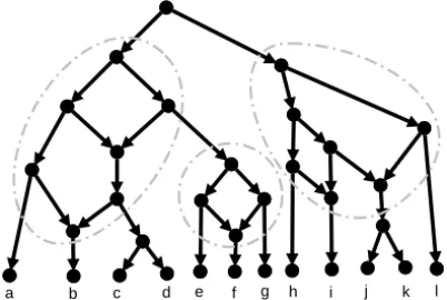
growing interest in extending this model to also incorporate non-treelike evo-lutionary phenomena such as hybridizations, recombinations and horizontal gene transfers. This has subsequently stimulated research into rooted phyloge-netic networks which generalize rooted phylogephyloge-netic trees by also permitting nodes with indegree two or higher, known as reticulation nodes, or simply reticulations. For detailed background information on phylogenetic networks we refer the reader to [15, 22, 24, 14, 29, 16]. Figure 1 shows an example of a rooted phylogenetic network.
a b c d e f g h i j k l
Fig. 1 Example of a phylogenetic network with five reticulations. The encircled subgraphs form its biconnected components, also known as its “tangles”. This binary network has level equal to 2 since each biconnected component contains at most two reticulations.
We are interested in the following biologically-motivated optimization prob-lem. We are given a set C of clusters on X , where a cluster is simply a strict subset of X . We wish to construct a phylogenetic network that “represents” all the clusters in C such that the amount of reticulation in the network is “mini-mized”. There are several different definitions of “represents” and “minimized” present in the literature. In this article we will consider only the softwired def-inition of “represents” [14, 31, 15, 16]. Most of our formal defdef-initions will be deferred to the preliminaries. Nevertheless, it is helpful to already formally state that a rooted phylogenetic tree T on X represents a cluster C ⊂ X if T contains an edge (u, v) such that C is exactly equal to the subset of X reachable from v by directed paths. A phylogenetic network N on X , on the other hand, represents a cluster C ⊂ X in the softwired sense if there exists some rooted phylogenetic tree T on X such that T represents C and T is topologically em-bedded inside N . Regarding “minimized”, we consider two closely related, but subtly different, variants of minimality. The first variant, reticulation number minimization, aims at minimizing the total number of reticulation nodes in the network1. The second, less well-known variant, level minimization [19, 18,
1 This is the definition when all reticulation vertices have indegree-2, for more general networks reticulation number is defined slightly differently. See the Preliminaries for more information.
27, 30, 26], asks us to minimize the maximum number of reticulation nodes contained in any “tangled” region of the network, which correspond to the non-trivial biconnected components of the underlying undirected graph (see Figure 1). The reticulation number is a global optimality criterion, while the level is a local optimality criterion. In general minimizing for one variant does not induce minimum solutions for the other variant (see e.g. [14, Figure 3]), although the algorithmic techniques used to tackle these problems are often related [20]. Both these problems are NP-hard and APX-hard [3, 29]. This raises the natural question: given a set of clusters C and a fixed integer r, is it NP-hard to determine whether or not there exists a network with reticulation number (respectively, level) equal to r representing C?
Prior to this article there were only partial answers known to these ques-tions. In [20] it was proven that the level-oriented question can be answered in polynomial time if the level is fixed. A striking aspect of this proof is that the running time of the algorithm is only polynomial time in a highly theoretical sense: it is too high to be of any practical interest. This exorbitant running time has two causes. Firstly, the exhaustive enumeration of all level-k genera-tors [27], essentially the set of all possible underlying topologies of a network constituted of a biconnected component if the taxa are ignored. Secondly, after determining the correct generator, a second wave of exhaustive enumeration determines where a critical subset of X should be located within the network, after which all remaining elements of X can easily be added without much computational effort.
The question of whether a corresponding positive result would hold for reticulation number minimization was left open, although the emergence of several partial results and practically efficient algorithms [14, 20] suggested that this might well be the case. Furthermore, it was not obvious how the algorithm from [20] could be adapted to yield a fixed parameter tractable algorithm for level minimization – where the parameter is the level of the network k – since k appears as an exponent of |X | in the running time of the algorithm. (We refer to [7, 23, 6, 11] for an introduction to fixed parameter tractability). Curiously, the main problem is not the enumeration of the gen-erators, because the number of generators is independent of |X | [8], but the allocation of the critical initial subset of taxa to their correct location in the network.
In this article we settle all these questions by proving for the first time that both level minimization and reticulation number minimization are fixed parameter tractable (where, in the case of reticulation number minimization, the parameter is the reticulation number of the whole network). We give one algorithm for level minimization and one algorithm for reticulation minimiza-tion, although the two algorithms have a large common core. The algorithms again rely heavily on generators, which we extend here to also be useful in the context of reticulation number minimization; generators had hitherto only appeared in the level minimization literature. In both algorithms the major non-triviality is showing how the network structure can still be adequately
recovered if the parameter is no longer allowed to appear in the exponent of |X | as it was in [20].
1.2 Beyond softwired clusters: the wider context
We believe that this approach is significant beyond the softwired cluster liter-ature. Other articles discuss the problem of constructing rooted phylogenetic networks not by combining clusters but by combining triplets [28, 30], charac-ters [12, 13, 35, 21] or entire phylogenetic trees into a network. These models are in general mutually distinct although they do have a significant common overlap which reaches its peak in the case of data derived from two phyloge-netic trees. To see this, note that if one takes the union of clusters represented by a set of two or more phylogenetic trees, then the reticulation number (or level) required to represent these clusters is in general less than or equal to the reticulation number (or level) required to topologically embed the trees themselves in the network, and this inequality is often strict. However, in the case of a set comprising exactly two trees the inequality becomes equality [29]. Hence for data obtained from two trees one could solve the reticulation number minimization and level minimization problems for clusters by using algorithms developed for the problem of topologically embedding the trees themselves into a network. These algorithms are highly efficient and fixed parameter tractable in a practical, as opposed to solely theoretical sense [1, 2, 5, 33]. However, these tree algorithms do not help us with more general cluster sets, because for more than two trees the optima of the cluster and tree models start to di-verge. Indeed, the cluster model often saves reticulations with respect to the tree model by weakening the concept of “above” and “below” in the network, which is exactly why the input tree topologies do not generally survive if one atomizes them into their constituent clusters [29]. Moreover, the literature on embedding three or more trees into a network is not yet mature, with articles restricting themselves to preliminary explorations [34, 17, 4]. It therefore seems plausible that the generator approach might be adapted to the tree model (or the other constructive methods mentioned) to yield a unified technique for producing positive complexity results for reticulation number minimization and level minimization, even in the case of many input trees (or data obtained from many input trees).
2 Preliminaries
Consider a set of taxa X , where |X | = n. A rooted phylogenetic network (on X ), henceforth network, is a directed acyclic graph with a single node with inde-gree zero (the root ), no nodes with both indeinde-gree and outdeinde-gree equal to 1, and nodes with outdegree zero (the leaves) bijectively labelled by X . In this article we usually identify the leaves with X . The indegree of a node v is denoted δ−(v) and v is called a reticulation if δ−(v) ≥ 2, otherwise v is a
tree node. An edge (u, v) is called a reticulation edge if its target node v is a reticulation and is called a tree edge otherwise. When counting reticulations in a network, we count reticulations with more than two incoming edges more than once because, biologically, these reticulations represent several reticulate evolutionary events. Therefore, we formally define the reticulation number of a network N = (V, E) as
r(N ) = X v∈V :δ−(v)>0
(δ−(v) − 1) = |E| − |V | + 1 .
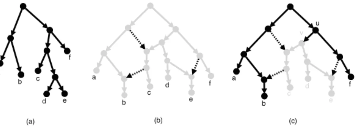
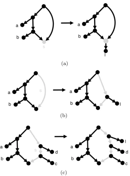
A rooted phylogenetic tree on X , henceforth tree, is simply a network that has reticulation number zero. We say that a network N on X displays a tree T if T can be obtained from N by performing a series of node and edge deletions and eventually by suppressing nodes with both indegree and outdegree equal to 1, see Figure 2 for an example. We assume without loss of generality that each reticulation has outdegree at least one. Consequently, each leaf has indegree one. We say that a network is binary if every reticulation node has indegree 2 and outdegree 1 and every tree node that is not a leaf has outdegree 2.
Proper subsets of X are called clusters, and a cluster C is a singleton if |C| = 1. We say that an edge (u, v) of a tree represents a cluster C ⊂ X if C is the set of leaf descendants of v. A tree T represents a cluster C if it contains an edge that represents C. It is well-known that the set of clusters represented by a tree is a laminar family, often called a hierarchy in the phylogenetics literature, and uniquely defines that tree. We say that a network N represents a cluster C “in the softwired sense” if N displays some tree T on X such that T represents C, see Figures 2 and 3. In this article we only consider the soft-wired notion of cluster representation and henceforth assume this implicitly2. A network represents a set of clusters C if it represents every cluster in C (and possibly more). The set of all softwired clusters represented by a network can be obtained as follows. For a network N , we say that a switching of N is obtained by, for each reticulation node, deleting all but one of its incoming edges. Given a network N and a switching TN of N , we say that an edge (u, v) of N represents a cluster C w.r.t. TN if (u, v) is an edge of TN and C is the set of labelled leaf descendants of v in TN. The set of all softwired clusters represented by N , denoted C(N ), is the set of clusters represented by all edges of N w.r.t. TN, where TN ranges over all possible switchings [15]. Note that every tree displayed by N corresponds to one or more switchings of N . It is also natural to define that an edge (u, v) of N represents a cluster C if there exists some switching TN of N such that (u, v) represents C w.r.t TN. Note that, in general, an edge of N might represent multiple clusters, and a cluster might be represented by multiple edges of N .
Given a set of clusters C on X , throughout the article we assume that, for any taxon x ∈ X , C contains at least one cluster C containing x and that C contains at least one non singleton cluster3 . For a set C of clusters on X we
2 Alternatively, we say that a network N represents a cluster C ⊂ X “in the hardwired sense” if there exists a tree edge (u, v) of N such that C is the set of leaf descendants of v.
a b c d e f a b c d e f a b c d e f (a) (b) (c) u v
Fig. 2 A phylogenetic tree T (a) and a phylogenetic network N (b,c); (b) illustrates in grey that N displays T (deleted edges are dashed); (c) illustrates that N represents (amongst others) the cluster {c, d, e} in the softwired sense (dashed reticulation edges are “switched off”).
define r(C) as min{r(N )|N represents C} and we refer to this as the reticula-tion number of C. The related concept of level requires some more background. A directed acyclic graph is connected (also called “weakly connected”) if there is an undirected path (ignoring edge orientations) between each pair of nodes. A node (edge) of a directed graph is called a cut-node (cut-edge) if its re-moval disconnects the graph. A directed graph is biconnected if it contains no cut-nodes. A biconnected subgraph B of a directed graph G is said to be a biconnected component if there is no biconnected subgraph B0 6= B of G that contains B. A phylogenetic network is said to be a level- ≤ k network if each biconnected component has reticulation number less than or equal to k.4 A network is called simple if the removal of a cut-node or a cut-edge creates two or more connected components of which at most one is non-trivial (i.e. con-tains at least one edge). A (simple) level-≤ k network N is called a (simple) level-k network if the maximum reticulation number among the biconnected components of N is precisely k. For example, the network in Figure 1 is a level-2 network (which is not simple), the network in Figure 3(a) is a simple level-4 network and the network in Figure 3(b) is a simple level-2 network. Note that a tree is a level-0 network. For a set C of clusters on X we define the level of C, denoted l(C), as the smallest k ≥ 0 such that there exists a level-k network that represents C. It is immediate that for every cluster set C it holds that r(C) ≥ l(C), because a level-k network always contains at least one biconnected component containing k reticulations.
We say that two clusters C1, C2 ⊂ X are compatible if either C1∩ C2 = ∅ or C1 ⊆ C2 or C2 ⊆ C1, and incompatible otherwise. Consider a set of clus-ters C. The incompatibility graph IG(C) of C is the undirected graph (V, E) that has node set V = C and edge set E = {{C1, C2} | C1 and C2 are incompatible clusters in C}. We say that a set of taxa X0⊆ X is compatible with C if X0= X or every cluster C ∈ C is compatible with X0, and incompatible otherwise.
4 Note that to determine the reticulation number of a biconnected component, the inde-gree of each node is computed using only edges belonging to this biconnected component.
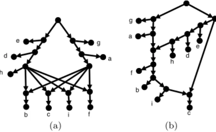
e d h b c i f g a (a) g a h d e f b i c (b)
Fig. 3 Two examples of networks that represent, among others, the set of clusters C = {{a, b, f, g, i}, {a, b, c, f, g, i}, {a, b, f, i}, {b, c, f, i}, {c, d, e, h}, {d, e, h}, {b, c, f, h, i}, {b, c, d, f, h, i}, {b, c, i}, {a, g}, {b, i}, {c, i}, {d, h}}. The network in (a) is a simple level-4 network, and the network in (b) is a binary simple level-2 network.
We say that a set of clusters C on X is separating if it is incompatible with all sets of taxa X0 such that X0⊂ X and |X0| ≥ 2.
When we write f (k) we mean “some function that only depends on k”. For simplicity we overload f (k) to refer to multiple different functions with this property. We write poly(n) to mean “some function f (n) that is polynomial in n”, where |X | = n. As in the case of f (k), we often overload this expression. Indeed, the goal of this article is not to derive exact expressions for the running time, but to show that it is bounded above by f (k)·poly(n). It should be noted that the f (k) that we encounter in this article can be extremely exponential in k. Also, |C| can in general be exponentially large as a function of n, but (as we shall see in due course) we may assume that |C| is bounded above by f (k) · poly(n) when the parameter k (reticulation number or level) is fixed. This is indeed obvious for the reticulation number and will be shown to be also true for the level in Section 3.2. The next lemma ensures that, if our goal is to find a network representing a set of clusters and minimizing the level or the reticulation number, we can restrict our attention to binary networks:
Lemma 1 [20] Let N be a network on X . Then we can transform N into a binary network N0 such that N0 has the same reticulation number and level as N and all clusters represented by N are also represented by N0.
It is well-known that for every set of taxa X , it is possible to construct a binary network with at most |X | − 1 reticulations which represents every possible cluster on X [29]. This implies that r(C) and l(C) are well defined for any set of clusters C. Thanks to this observation and to Lemma 1, there exists a binary network N with reticulation number r(C) (or with level l(C) if we are interested in level minimization) that represents C. We henceforth restrict our analysis to binary networks and, except in places where it might cause confusion to not be explicit, we will not emphasize again that we only deal with this kind of network.
3 Minimizing level is fixed parameter tractable
The aim of this section is to show that level-minimization is fixed parameter tractable. To compute l(C), we will repeatedly query, “Is l(C) = k? If so, construct a network with level equal to k that represents C”, where k starts at 0 and is incremented by 1 until the query is answered positively. Assuming that the queries are correctly answered, this process will terminate after l(C) + 1 iterations. Hence, to prove an overall running time of f (l(C)) · poly(n), it is sufficient to show that for each k we can correctly answer the query in time at most f (k) · poly(n). Note that r(C) = l(C) = 0 if and only if all the clusters in C are pairwise mutually compatible, which can be easily checked in time poly(n), so we henceforth assume that k ≥ 1.
The high-level idea is the following. In [31, 15] it is shown that level-k net-works can be constructed using a divide and conquer strategy. Informally, the idea is to construct a level-≤ k network for each connected component of the incompatibility graph IG(C) and then to combine these into a single network. The clusters in each connected component first have to be processed, which creates (for each component) a separating set of clusters. From Lemma 1 of [20], we know that, if a level-k network representing a separating set of clusters C on X exists, a simple level-k network representing C has to exist. Moreover, the transformation underpinning Lemma 1 allows us to assume that this simple level-k network is binary. Hence, the divide and conquer strategy essentially reduces to constructing binary simple level-≤ k networks for separating sets of clusters (and then combining them into a single network).
In Section 3.1 we show how to construct a simple level-k network in time f (k)·poly(n) from a separating set of clusters. Subsequently we show in Section 3.2 how to combine these networks in time f (k) · poly(n) into a single level-k network.
3.1 Constructing simple networks from separating cluster sets
Before proving the main result of this paper, we need to prove some preliminary results.
Proposition 1 Given a simple level-k network N and a set of clusters C on X , checking whether C is represented by N can be done in time f (k) · poly(n), where n = |X |.
Proof. Note that a simple level-k network contains exactly k reticulations. Thus, there are at most 2k trees displayed by N and each tree represents at most 2(n − 1) clusters. This means that |C(N )| is at most 2k+1(n − 1). Since N cannot represent C if |C| > |C(N )|, checking whether C ⊆ C(N ) takes at most f (k) · poly(n) time.
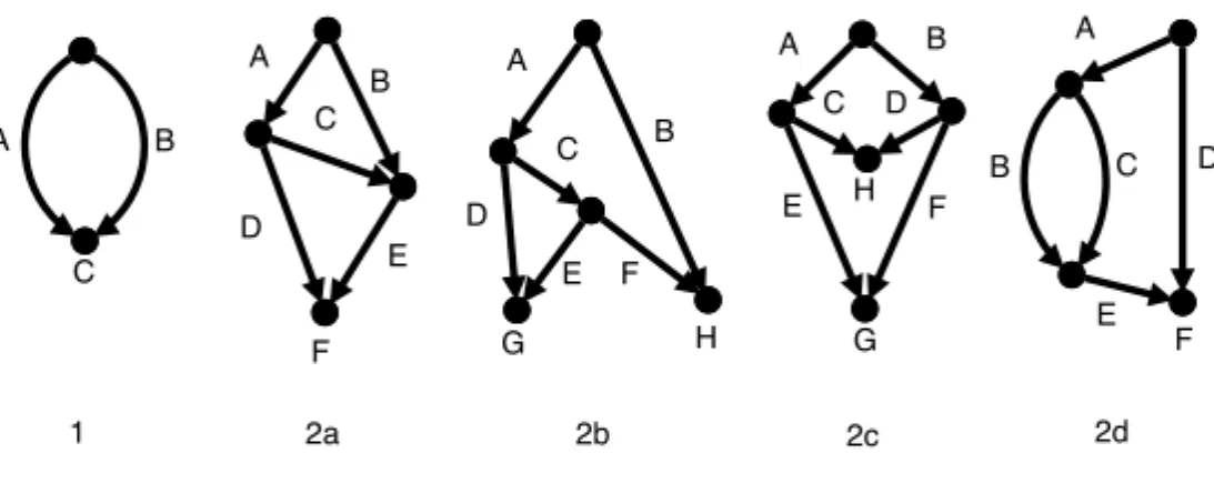
A B C A B C D E F A B C D E F G H A B C D E F G H A B C D E F 1 2a 2b 2c 2d
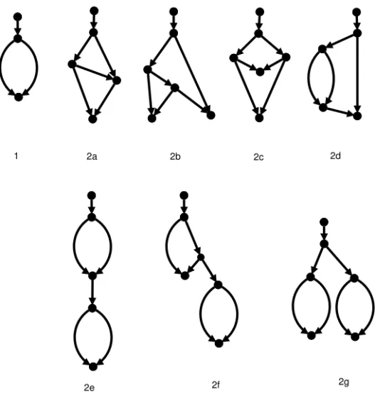
Fig. 4 The single level-1 generator and the four level-2 generators. Here the sides have been labelled with capital letters.
Thus, if |C| > 2k+1(n − 1), since C is assumed to be separating, it is not possible that l(C) = k and we can immediately answer “no” to the query5. We thus henceforth assume that |C| ≤ 2k+1(n − 1) i.e. that C contains at most f (k) · poly(n) clusters.
If all the leaves of a binary simple level-k network N are removed and all nodes with both indegree and outdegree equal to 1 are suppressed, the result-ing structure is called a level-k generator as defined in [27]. See Figure 4 for the level-1 and level-2 generators. The number of level-k generators is bounded by f (k) [8]6.
The sides of a level-k generator are defined as the union of its edges (the edge sides) and its nodes of indegree-2 and outdegree-0 (the node sides). The number of sides in a generator is bounded by f (k), because the sum of its vertices and edges is linear in k [30].
Definition 1 The set Nk (for k ≥ 1) is defined as the set of all networks that can be constructed by choosing some level-k generator G and then applying the following leaf hanging transformation to G such that each taxon of X appears exactly once in the resulting network. (This is essentially identical to the definition given in [30], which is only a superficial refinement of the definition given in [27]).
1. First, for each pair u, v of vertices in G connected by a single edge (u, v), replace (u, v) by a path with l ≥ 0 internal vertices and, for each such internal vertex w, add a new leaf w0, an edge (w, w0), and label w0 with some taxon from X . All the taxa added in this way are “on side s” where s is the side corresponding to the edge (u, v). (It is also permitted that the path has zero internal nodes i.e. that the side remains empty).
5 Recall that, by Lemma 1 of [20], the existence of a level-k network representing a sep-arating set of clusters C on X implies that a simple level-k network representing C has to exist.
6 Note that the number of level-k generators grows rapidly in k, lying between 2k−1 and k!250k[8].
2. Second, for each pair u, v of vertices in G connected by two edges, treat the two edges as in step 1, but ensure that at least one of the two paths does not have zero internal nodes.
3. Third, for each vertex v of G with indegree 2 and outdegree 0 add a new leaf y, an edge (v, y) and label y with a taxon x ∈ X ; we say “taxon x is on side s” where s is the side corresponding to vertex v.
The main reason for step 2 in Definition 1 is to ensure that multi-edges in generators do not survive in the final network, since our definition of phylo-genetic network does not allow multi-edges. The next lemma follows directly from the results in Section 3.1 of [27]:
Lemma 2 The set Nk (for k ≥ 1) is equal to the set of all binary simple level-k networks.
For example, the simple network in Figure 3(b) has been obtained from generator 2a (see Figure 4) by putting 0 taxa on sides A and D, 1 taxon on side F , 2 taxa on side B and 3 taxa on sides C and E.
By Lemma 1 of [20] and Lemmas 1 and 2, we have the following:
Corollary 1 Let C be a separating set of clusters on X such that l(C) ≥ 1. Then there exists a network N in Nl(C) such that N represents C.
Given a taxon set X , we call any network resulting from adding all taxa in X to sides of a generator G (in the sense of Definition 1) a completion of G on X . Here we call a side that receives ≥ 2 taxa a long side, a side that receives 1 taxon a short side and a side that receives 0 taxa an empty side. Figure 3(b) is thus a completion of generator 2a, where sides A and D are empty, side F is short, and sides B, C, E are long. Note that in simple networks node sides (such as F in the example) are always short. Indeed, they cannot be empty – otherwise they will violate the definition of a network – and they cannot be long, since simple networks never have two or more taxa with the same parent [20].
Given a generator G, we call a set of side guesses for G, denoted by SG, a set of guesses about the type of each side of G (i.e. whether it is empty, short, or long). A completion N of G on X respects SGif all sides that are long in SG receive at least 2 taxa in N , sides that are short in SG one taxon and empty sides zero taxa. Then we have the following result:
Observation 1. Searching in the space of all binary simple level-k networks on X is equivalent to searching in the space of all completions of a level-k generator G respecting a set of side guesses SG, iterating overall all sets of side guesses for a generator and all level-k generators.
Let G be a level-k generator and let SG be a set of side guesses for G. We say that the pair (G, SG) is side-minimal w.r.t. a separating cluster set C on X and an integer k, if there exists a completion N of G on X respecting SG that is a level-k network representing C and, amongst all simple level-k networks that represent C, N has a minimum number of long sides, and (to
further break ties) amongst those networks it has a minimum number of short sides.
We define an incomplete network as a generator G, a set of side guesses SG, a set of finished sides (i.e. those sides for which we have already decided that no more taxa will placed on them), a set of future sides (i.e. those short and long sides that have had no taxa allocated yet), at most one long side – the active side – on which at least one taxon has already been placed but where we might still want to add some more taxa, and information describing the position of already-allocated taxa on the finished and active sides. A valid completion of an incomplete network is an assignment of the unallocated taxa to the future sides and (possibly) above the taxa already placed on the active side, that respects SG and such that the resulting network (which we call the result of the valid completion) represents C. Informally, the result of a valid completion is any network on X respecting SG and representing C that is obtained by respecting all placements of taxa made thus far.
For example, consider again the network in Figure 3(b). Let N be the net-work in that figure and let N0 be the network obtained from N by deleting taxa c, d, e and suppressing the resulting vertices with indegree and outdegree both equal to 1. Let G be generator 2a, and let SG be the set of side-guesses where sides A and D are empty, side F is short, and sides B, C, E are long. Then N0 is an incomplete network for (G, S
G) where sides A, B, D, E are fin-ished, F is a future side and C is the active side. We can perform a valid completion of N0 by putting taxa d and e above taxon h on side C and then putting c on side F . In this case, N is the result of the completion, although in general an incomplete network might have many valid completions, or none. Given a cluster set C, we write x →C y if and only if every non-singleton cluster in C containing x, also contains y. Then we have the following result. Proposition 2 Given a separating set of clusters C on X and an ordered set of distinct taxa of X (x1, . . . , xj) such that j ≥ 2 and xi →C xi+1 for 1 ≤ i ≤ (j − 1). Then xj 6→C x1.
Proof. If xi→C xi+1for 1 ≤ i ≤ (j − 1) and xj→C x1, this means that the set X0 = ∪j
i=1xi is compatible with C. Note that we can have that X0 = X only if all clusters in C are singleton clusters, but this is not possible (see footnote 3). So X0⊂ X and thus, since |X0| ≥ 2, we have a contradiction.
The following observations will be useful to prove Lemma 3.
Observation 2. Let N be a phylogenetic network on X representing a set of clusters C on X constructed by choosing some level-k generator G and then applying the leaf hanging transformation described in Definition 1 to G. If two taxa x and y in X are on the same side of the generator underlying N and the parent of x is a descendant of the parent of y, then y →C x.
Given a simple phylogenetic network N , we say that a side s0 is reachable from a side s in N if there is a directed path in the generator underlying N from the head of side s to the tail of side s0.
Observation 3. Let N be a phylogenetic network on X representing a set of clusters C on X constructed by choosing some level-k generator G and then applying the leaf hanging transformation described in Definition 1 to G. More-over, let x and y be two taxa of X on the same side s of the generator under-lying N such that y →C x and let z be a taxon on a side s0 6= s such that s0 is not reachable from s and z →C x. Then we have that z →C y.
Proof. Since z →C x, we know that every non-singleton cluster that contains z also contains x. Now, let C such a cluster. C is represented by some tree T displayed by N , so some edge e in T is such that C is the set of all taxa reachable from directed paths from the head of e. Now, z and x are both in C, so there is a directed path from the head of e to z and a directed path from the head of e to x. Since s0 is not reachable from s, the only way that such a directed path can reach x is via the parent of y, hence the fact that z →C y. If no cluster C containing z and x exists, since z →C x we have that the only cluster containing z is the singleton cluster {z}. Then, obviously, z →C y too.
Observation 4. Let N be a phylogenetic network on X representing a set of clusters C on X constructed by choosing some level-k generator G and then applying the leaf hanging transformation described in Definition 1 to G. Let x and y be two taxa in X on the same side s of the generator underlying N such that there exists an edge e from the parent of y to the parent of x. Then e represents all clusters in C containing x but not y.
Observation 5. Let C be a separating cluster set on X . Then every size-2 subset of X is incompatible with C.
Let N be a simple phylogenetic network, l a taxon and s a side of the generator G underlying N . We denote by N (l, s) the following operations: If s is a short side, then N (l, s) is simply the network obtained by putting l on side s (in the sense of Definition 1). Otherwise, s is a long side, and then N (l, s) is the network obtained by placing l “just above” the highest taxon on side s. If there are not yet any taxa on side s then we simply let l be the first taxon on side s. (See Figure 5 for clarification). Note that we exclude from consideration the case where s is a short side that already has a taxon on it.
The core of our proof of fixed-parameter tractability relies on Algorithm 1 (see pseudocode). Let us assume that we have an incomplete network N with an active side s (which is by definition long) such that all long sides s0 6= s that are reachable from s, are finished. (These preconditions will be motivated in due course.) Informally, Algorithm 1 identifies and returns a set of possible next steps in constructing a valid solution. It decides whether to terminate the side s (and declare it finished), or to add a single new taxon to the top of it. In the case that it decides to add a taxon, it has to decide which specific taxon to add. Furthermore, when this taxon is added, it can force some other taxa to be allocated to unfinished short sides that are “beneath” s, and the algorithm also has to decide how to allocate these taxa. In this way, Algorithm 1 can
a b s a b l (a) a b l a b s (b) a b s c d a b c d l (c)
Fig. 5 Three examples of the N (l, s) operation. (a) N (l, s) when s is an unfinished short node side; (b) N (l, s) when s is an unfinished short edge side (or a long side that does not yet have any taxa); (c) N (l, s) when s is a long side that already has at least one taxon.
also cause some short sides to be allocated a taxon, although the algorithm itself is only applied to long sides7.
Lemma 3 Let C be a separating set of clusters on X and let k be the first in-teger for which a level-k network representing C exists. Let N be an incomplete network such that its underlying generator G and set of side guesses SG are such that (G, SG) is side-minimal w.r.t. C and k, and let s be the active side of N . Then, if a valid completion for N exists, Algorithm 1 computes a set of (incomplete) networks N such that this set contains at least one network for which a valid completion exists.
Proof. Recall that, from Corollary 1, we can restrict our search to networks in Nk. We write X (N ) to denote the set of taxa present in a (incomplete) network N . For a set of clusters C on X and a subset X0 ⊆ X , we define the restriction of C to X0 as {C ∩ X0|C ∈ C}. We start the proof by analyzing the case when U = ∅ (see Algorithm 1 for the definition of X0, U , B(l), etc).
7 Indeed, short sides can only be allocated taxa in two ways. Firstly, indirectly via Algo-rithm 1. Secondly, when there are no longer any unfinished long sides, at the very end of the entire procedure, in Algorithm 3.
Algorithm 1 addOnSide(N, s)
1: X0← X \ X (N );
2: xi← the most recent taxon inserted on side s; 3: L ← {l ∈ X0| l →Cxi};
4: L0← {l ∈ L| there does not exist l0∈ L such that l06= l and l →Cl0}; 5: U ← {s0|s06= s is a side of N that is not yet finished and is reachable from s}; 6: for l ∈ L0do
7: S(l) =S{C ∈ C| xi∈ C and l 6∈ C};
8: B(l) = X0∩ S(l). 9: if U = ∅ then
10: if |L0| 6= 1 then declare s as finished in N and return N ; 11: l ← removeFirst(L0);
12: if B(l) 6= ∅ then declare s as finished in N and return N ; 13: if N (l, s) does not represent C restricted to X (N ) ∪ {l} then
14: declare s as finished in N and return N ;
15: else return N (l, s); 16: else
17: if L0= ∅ then
18: declare s as finished in N and return N ;
19: if |L0| ≥ 2 then
20: N ← N , where s is declared as finished;
21: if |L0| ≤ |U | then
22: N0← the set of networks obtainable from N by allocating all taxa in L0
to sides in U ;
23: N ← N ∪ N0;
24: if |L0| − 1 ≤ |U | then
25: for l ∈ L0do
26: N0← the set of networks obtainable from N (l, s) by allocating all taxa
in L0\ {l} to sides in U ; 27: N ← N ∪ N0; 28: return N ; 29: if |L0| = 1 then 30: l ← removeFirst(L0); 31: if B(l) 6= ∅ then
32: N ← N , where s is declared as finished;
33: for each side s0∈ U do
34: N ← N ∪ {N (l, s0)};
35: if |B(l)| ≤ |U | then
36: N0 ← the set of all networks obtainable from N (l, s) by allocating all
taxa in B(l) to sides in U ;
37: N ← N ∪ N0;
38: else
39: if N (l, s) does not represent C restricted to X (N ) ∪ {l} then
40: N ← N , where s is declared s as finished;
41: for each side s0∈ U do
Case U = ∅. Suppose |L0| 6= 1. If |L0| = 0 then there are two possibilities. If L = ∅ then clearly no taxon l can be placed directly above xion s, because that would mean l →C xi, and thus l ∈ L, contradiction. Hence the only correct move is to declare that the side s is finished and return N . If L 6= ∅ then, since |L0| = 0, we have that, for every l ∈ L there exists some l0∈ L such that l 6= l0 and l →C l0. Clearly the →C relation is not allowed to create cycles in L,
42: N ← N ∪ {N (l, s0)};
43: else
44: D ← an arbitrary set of |U | taxa such that D ∩ X = ∅;
45: N∗(l, s) ← a network obtained from N (l, s) by arbitrarily and bijectively
assigning each taxon in D to a side in U ;
46: C ← {C ∈ C such that x¯ i∈ C, l 6∈ C, and C ⊆ X (N )};
47: if N∗(l, s) does not represent ¯C then
48: N ← N , where s is declared s as finished;
49: for each side s0∈ U do
50: N ← N ∪ {N (l, s0)};
51: else
52: N ← N (l, s);
53: return N ;
because otherwise the set of taxa in the cycle would form a cluster compatible with C (see Proposition 2). Suppose we start at an arbitrary taxon in L and perform a non-repeating walk on the taxa of L by following the →C relation. Given that L is of finite size and this walk cannot visit a taxon of L that it has already visited earlier in the walk (thus creating a cycle), we will find a taxon l ∈ L such that there is no l0∈ L such that l 6= l0 and l →
C l0, meaning that l ∈ L0, contradiction. So the case that L 6= ∅ but L0= ∅, cannot actually happen. Now, consider the case that |L0| ≥ 2. Algorithm 1 will always end the side s and return N in this case. Indeed, no valid completion of N can have some taxon p that has not yet been allocated above xion side s. Suppose this is not true. Clearly, from Observation 2, p →C xi, so p ∈ L. In this case, all taxa in L0 are either equal to p, or underneath p and above xi. Indeed, let l 6= p be a taxon in L0 and suppose, for the sake of contradiction, that l is above p on side s or on another side s0. If l is above p on side s, then from Observation 2 we have that l →C p. If l is on another side s0, the fact that |U | = 0 implies that there is no room under side s so, by Observation 3 we have that l →C p. Thus, in both cases (i.e. if l is above p on side s or on a different side s0) we have that l →
C p, meaning that l 6∈ L0, contradiction. We can hence conclude that each taxon in L0 is either equal to p, or underneath p and above xi in any completion of N where p is on s. But, however one arranges two or more taxa on one side, at least one taxon will imply another taxon in the sense of the →C relation. More formally, in any case there exist two taxa l and l0 in L0 such that l 6= l0 and l →C l0. This implies that l 6∈ L0, contradiction. This concludes the correctness of the case |L0| 6= 1.
We now consider the case when |L0| = 1. Let l be the only taxon in L0. In this case, Algorithm 1 will return N if B(l) 6= ∅. Indeed, no valid completion of N exists where one or more taxa are placed above xi on s. Suppose this is wrong. In that case, observe that in every valid completion l always has to be the taxon directly above xi. Indeed, if there was some valid completion such that l is not directly above xi, then there would exist some taxon l0 6= l such that l0 →C xi (from Observation 2) and l →C l0 (as before, this follows from the fact that U = ∅ and from Observations 2 and 3). This would mean that l 6∈ L0, contradiction. So we assume that l is directly above xi. Now,
since B(l) 6= ∅, there is some cluster in the input that contains xi, does not contain l, and contains some not-yet allocated taxon distinct from l. From Observation 4, the only edge that can represent such a cluster is the edge e between the parents of xi and l. But all the clusters represented by e consist only of already-allocated taxa, because U = ∅. This means that adding l on side s will only lead us to construct non-valid completions. Hence we conclude that, if B(l) 6= ∅, all valid completions of N do not contain any other taxon on s and ending the side s is the right choice.
Now consider the case B(l) = ∅ and let C0 be C restricted to X (N ) ∪ {l}. If N (l, s) does not represent C0 we are definitely correct to declare the side s as finished and return N . Indeed, all valid completions of N do not contain any other taxon on s. Suppose it is not correct. Then there exists a valid completion of N where at least one taxon is above xi on s. Again, for the same reasons as above we assume that l is always the taxon directly above xi. Since N (l, s) does not represent C0, and this incompatibility cannot be eliminated by adding more taxa, we conclude that there are no valid completions of N with taxa above xion side s. Hence, ending the side s is the only correct option. Suppose now that N (l, s) does represent C0; Algorithm 1 adds l above xi on side s, and does not declare s as finished. This conclusion can only be incorrect if all valid completions require that l is not directly above xi. We observe that in any valid completion of N there can be no taxon l06= l directly above xi on s, because otherwise, as before, since U = ∅ we will have that l →C l0→C xi and hence l 6∈ L0, contradiction. So all valid completions terminate the side at xi. Let N0 be an arbitrary valid completion of N and denote by N00the network obtained from N0 by moving l, wherever it is, just above xi. Firstly, we claim that N00 still represents C. Recall that l →C xi, so the only potential problem is with clusters in C that contain xi but do not contain l. Let C be such a cluster not represented by N00. Suppose C 6⊆ X (N ) ∪ {l}. But in this case we would have B(l) 6= ∅ in N , contradiction. So the only possibility is that C ⊆ X (N ) ∪ {l}. Clearly C was in C0 and was thus represented by N (l, s). Moreover, from Observation 4, the edge that represents C in N (l, s) is the edge between the parents of l and xi. Given that U = ∅, no more taxa can be added “underneath” side s and this edge still represents C in N00 because N0 is a valid completion of N . Hence moving l in the way is safe in terms of cluster representation.
Secondly, we claim that moving l in this way does not alter the side types i.e. the empty/short/long sides before moving l remain empty/short/long after moving l. To see this, note that moving l from its original location reduces the number of taxa by 1 on some side, and increases the number of taxa of s by 1. Side s is by assumption already long, so remains so. The side of N0containing l cannot change from being long to being short in N00, because this lowers the total number of long sides, and by assumption the pair (G, SG) underlying N is side-minimal. Similarly it cannot change from being short to being empty, because this leaves the number of long sides the same but reduces the number of short sides, again contradicting the assumption that (G, SG) is side-minimal. Combining these two claims - that moving l is safe for cluster representation
and does not alter the side types nor the underlying generator - let us conclude that there is a valid completion for N in which l is placed directly above xi. Hence it is correct to add l above xion side s, and not to declare s as finished. Case U 6= ∅. The case |L0| = 0 is identical to the corresponding subcase when U = ∅. This means that in this case it is always correct to declare the side s as finished and return N .
Consider now the case |L0| ≥ 2. Observe firstly that, if some taxon l ∈ L0 is placed directly above xi, then all remaining taxa in L0must be allocated to sides in U . To see why this is, note that for every l0∈ L0we have that l0 →
Cxi. So, if l0 6= l is placed above l on s or on a side not in U , then, from Observation 2 and 3 we would have that l0 →C l →C xi, contradicting the fact that l0 is in L0. We only need to show that, if a valid completion for N exists, then the set N contains a network for which there exists a valid completion. Note that N contains (line 20) N , where s is declared as finished, (lines 21-23) all possible networks obtained from N by allocating all taxa in L0 to sides in U and (lines 24-27) all possible networks obtained from N (l, s) by allocating all taxa in L0\ {l} to sides in U , iterating over all l ∈ L0. The only case that these three sets do not describe, is when every valid completion has a taxon p 6∈ L0directly above xi, but at least one taxon l ∈ L0 is not mapped to U . But this implies, similarly to the case |U | = 0, that l →C p →C xi, so l 6∈ L0, contradiction. Hence this case cannot happen, and the three sets actually describe all possible outcomes in this situation. So at least one of them will contain a network with a valid completion in the case N does have a valid completion.
Consider now the case |L0| = 1. We begin with the subcase B(l) 6= ∅. Similar to previous arguments we know that, if we place l (the only element in L0) directly above xi, all taxa in B(l) have to be allocated to U . This holds because, from Observation 4, any cluster that contains xi but not l is represented by the edge between the parents of l and xi. If B(l) 6= ∅, the set N is composed of (line 32) N , where s is declared as finished, (lines 33-34) all possible networks obtained from N by allocating l to a side in U and (lines 35-37) all possible networks obtained from N (l, s) by allocating all taxa in B(l) to sides in U . Observe that the only situation that these three guesses do not describe, is when some taxon p 6= l is placed above xiand l is not mapped to U . But in this case we would have that l →C p →C xi, contradicting the fact that l is in L0. So N does again describe all possible outcomes.
This leaves us with the very last subcase, |L0| = 1 and B(l) = ∅. The subcase when N (l, s) does not represent C restricted to X (N ) ∪ {l} is ac-tually fairly straightforward. It is clear that l cannot be placed in this position in a valid completion. Hence the only two situations that line 40 and lines 41-42 do not describe, is when some element p 6= l is placed directly above xi, and l is not mapped to U . But, as before, this implies that l →C p →C xi, which as we have seen is not possible. So the only remaining subcase is when |L0| = 1, B(l) = ∅ and N (l, s) does represent C restricted to X (N ) ∪ {l}. Now, consider the network N∗(l, s). Informally the dummy taxa in N∗(l, s) act as “placeholders” for taxa that will only later in the algorithm be mapped
to U . We do not know exactly what these taxa will be, but we know that they will definitely be there. Consider a cluster C ∈ ¯C. If N∗(l, s) does not represent C then this must be because of the dummy taxa, because we know that N (l, s) did represent C restricted to X (N ) ∪ {l}. Note that this holds irrespective of the true identity of the dummy taxa. Hence, C will never be represented by any completion of N (l, s). For this reason we conclude that, if N∗(l, s) does not represent ¯C, it is definitely correct to declare the side s finished (line 48) or allocate l to a side in U (lines 49-50).
Finally, suppose N∗(l, s) does represent ¯C. This is the flip-side of the pre-vious argument. Whatever the true identity of the dummy taxa, every valid completion of N (l, s) will represent every cluster in ¯C. Let N0 be an arbitrary valid completion of N and denote by N00 the network obtained from N0 by moving l, wherever it is, just above xi. Now, as we did earlier we argue that in this case it is “safe” to put l directly above xi. Indeed, because B(l) = ∅, the only clusters that might not be represented in N00 are clusters in ¯C. But we have shown that when l is placed directly above xi all the clusters in ¯C are represented regardless of how we complete the rest of the network. Sec-ondly, we argue just as before that moving l in this way cannot alter the side types. So if we place l on side s directly above xi there must still exist a valid completion. This concludes the proof of the lemma.
Algorithm 2 will repeatedly call Algorithm 1 until it finally declares the active side finished. The algorithm works with sets of networks because each execution of Algorithm 1 potentially returns a set of (incomplete) networks, reflecting the various different decisions that Algorithm 1 can make. Note that Algorithm 2 is only executed for long sides. Also, we note that during the execution of Algorithm 2 a call to Algorithm 1 might return a network in which the side s is finished but has fewer than two taxa on it. Such an outcome violates the assumption that side s is long. In such a case we can easily detect this and cease exploring this particular branch of the search tree. (Throughout the algorithms in this paper there are actually many such situations in which we can easily detect that we are exploring a wrong search path, and subsequently prune the search tree. However, to keep the exposition clear we have not discussed these explicitly).
Algorithm 2 completeSide(N, s)
1: N ← N ;
2: while there exists N ∈ N such that s is not finished in N do
3: N ← N \ N ;
4: N ← N ∪ addOnSide(N, s);
Lemma 4 Let C be a separating set of clusters on X and let k be the first in-teger for which a level-k network representing C exists. Let N be an incomplete network such that its underlying generator G and set of side guesses SG are such that (G, SG) is side-minimal w.r.t. C and k, and let s be the active side
of N that contains only a single taxon. Algorithm 2 computes in f (k) · poly(n) time a set of (incomplete) networks N for which s is a finished side, such that N contains at least one network for which there exists a valid completion (if any exists).
Proof. The correctness follows from Lemma 3. We now prove the running time. First, note that the size of the set N returned by Algorithm 1 is bounded by f (|U |). This is evident for the sets N constructed on lines 33-34, 41-42 and 49-50 but it holds also for the sets N0 constructed respectively on lines 21-23, 24-27 and 35-37, since these sets are constructed only if, respectively, |L0| ≤ |U |, |L0| − 1 ≤ |U | or |B(l)| ≤ |U |. Since in all other cases |N | = 1, the size of the set N returned by Algorithm 1 is indeed bounded by f (|U |). Since the number of sides in a generator is bounded by f (k) and U is a subset of the short sides of the generator (which follows from the fact that all long sides reachable from s are assumed to be finished), we have that |U | is bounded by f (k). From that and from Proposition 1, it follows that the running time of Algorithm 1 is f (k) · poly(n).
Second, note that, each time that Algorithm 1 returns a set of networks N such that |N | > 1, |U | decreases or s is declared as finished. Additionally, when U = ∅, then Algorithm 1 returns only one network per call and we have at most O(n) of these calls (because either s is declared finished or a new taxon is added to s). Since the search tree contains f (k) · poly(n) nodes and f (k) · poly(n) time is needed for each node of the search tree, the running time of Algorithm 2 is bounded by f (k) · poly(n).
We will subsequently use the term lowest side to denote an unfinished long side such that there is no other unfinished long side s0 6= s that is reachable from s. The following lemma is basically the fixed parameter tractable version of Lemma 3 from [20]. It proves that Algorithm 3, which is the top-level part of the overall procedure, is FPT. Informally, the algorithm guesses the backbone topology of the network we are constructing (i.e. the level-k generator); guesses which sides should be long, short or empty; repeatedly picks a long side to allocate taxa to; guesses the first taxon on that side; completes the side using Algorithm 2; and collapses the taxa on that side into a single meta-taxon once it is finished. When all long sides are finished, Algorithm 3 guesses how to allocate taxa to any remaining unfinished short sides.
Lemma 5 Let C be a separating set of clusters on X . Then, for every fixed k ≥ 0, Algorithm 3 determines whether a level-k network exists that represents C, and if so, constructs such a network in time f (k) · poly(n).
Proof. Algorithm 3 starts by choosing a level-k generator G and a set of side guesses SG ‘in increasing side order”, i.e. generators and sets of guesses are analyzed in such a way that generators with a smaller number of sides and sets of side guesses with a smaller number of long sides, and (to further break ties) short sides, are analyzed first. This implies that a side-minimal pair (G, SG), if any exists, is analyzed before any other pair (G0, SG0 ) for which a valid completion exists. This is done to be able to apply Lemma 4.
Then (see lines 4-18), the algorithm constructs a set of complete networks, i.e. simple level-k networks where each short side has received a single taxon and each long side at least two, and returns the first of them that represents C, if any exists.
Algorithm 3 ComputeLevel-k(C)
1: for each level-k generator G in increasing side order /* i.e. generators with a smaller number of sides are analyzed first */ do
2: for each set of side guesses SG in increasing side order /* i.e. sets of side
guesses with a smaller number of long sides, and (to further break ties) short sides, are analyzed first */ do
3: N ← (G, SG);
4: while there exists N ∈ N such that N contains a lowest side s do
5: N ← N \ N ;
6: for each l ∈ X (s) /* X (s) denotes the set of all taxa in X that
are candidates to be the first taxon on side s */ do
7: N0← completeSide(N (l , s), s);
8: N00← the networks in N0where s contains more than one taxon;
9: for each N ∈ N00do
10: collapse all taxa on side s into a single meta-taxon S and adjust the cluster
set accordingly;
11: N ← N ∪ N00;
12: if |N | > 0 then
13: while there exists N ∈ N do
14: de-collapse the collapsed sides;
15: N0 ← the set of networks obtainable from N by allocating the taxa in
X \ X (N ) to any short sides that have not yet been allocated a taxon;
16: if there is a network N0∈ N0 representing C then
17: return N0;
18: N ← N \ N ;
19: return ∅;
Note that lines 10 and 14 of the algorithm are only a technical step. Indeed, when we declare a side s as finished, we assume that we will never alter that side again. Hence it does not change the analysis if we collapse all the taxa on side s into a single meta-taxon. That is, if we have decided that the taxa on the side s are – from the bottom to the top – l , x1, . . . , xl we simply replace all these taxa by a single new taxon S and replace l , x1, . . . , xl by S in any clusters in C that they appear in (line 10). This collapsing step ensures that the set of sides reachable from the current lowest side are always empty or short sides. This will be helpful when proving the running time of Algorithm 3, see below. Note that C stays separating after the collapsing, since the taxa on s are such that xl→C . . . x1→C l . When we are finished allocating all the taxa in X and are ready to check whether the resulting final network represents C we can simply de-collapse all the S i.e. “unfold” all the long sides that we have collapsed (line 14). This means that the correctness of Algorithm 3 follows by Observation 1 and Lemma 4.
We now need to prove the correctness of the running time. First, note that the number of pairs (G, SG) to consider is bounded by f (k) since both the
number of generators and the number of sides per generator are bounded by f (k).
We now need to prove that the size of X (s) is at most f (k) for all sides s i.e. that the number of taxa that might be the first taxon l on side s, is not too big. So let l be any taxon which can fulfil this role, and let x be the taxon directly above l on side s. (The taxon x must exist because we assume that s is long). Clearly, x →C l . By line 10, we have that the only sides reachable from side s are short and empty sides. Moreover, we know from Observation 5 that, because C is separating, there is some non-singleton cluster C ∈ C such that l ∈ C but x 6∈ C. By Observation 4, such a cluster C has to be represented by the edge e between the parents of x and l . Now, any cluster represented by e can only contain taxa that are reachable from e by a directed path. The only sides that are reachable from side s are short and empty sides, so the cluster C can only contain at most f (k) taxa (because there are at most f (k) short sides). So we know that l is in some cluster C, and that C is “small” in the sense that its size is bounded above by f (k). So if we take all “small” clusters, and let X (s) be their union, we know that we could simply try taking every element in X (s) and guessing that it is equal to l . To ensure that we do not use too many guesses, we have to show that |X (s) | is bounded by f (k). To see that this holds, consider the question: how many taxa are only in clusters that contain at most c taxa? Observe that on every long side only the c taxa furthest away from the root are potentially in such clusters. Any taxon closer to the root on a long side cannot possibly be in a cluster of size at most c, because if it is in a cluster then so are at least c other taxa too. Hence there are at most f (k) taxa that can be involved in “small” clusters: the taxa on the short sides and the taxa at the bottom of the long sides. So we have that |X (s) | is bounded by f (k) and we can guess l with at most f (k) guesses.
The collapsing and de-collapsing steps (lines 10 and 14) can be done in f (k) · poly(n) time, as well as completing each side s (line 7), by Lemma 4. Moreover, by Proposition 1, also checking whether N represents C takes f (k) · poly(n) time. Additionally, the allocation of remaining taxa to the unfinished short sides (line 15) takes a time bounded by f (k). Indeed, if we have a number of not yet assigned taxa bigger than the number of unfinished short sides we can cease exploring this particular branch of the search tree. This means that, if the size of N is bounded by f (k), then the entire algorithm can be executed in f (k) · poly(n) time. And this is indeed the case, since |X (s) | and (summing over all iterations) the total number of lowest sides are bounded by f (k) and each time that a side is completed, the number of unfinished long sides decreases by 1.
A comment on the running time
We have shown that the running time of Algorithm 3 is at most f (k) · poly(n). We wish to emphasize that, due to the wholly theoretical nature of the al-gorithm, the f (k) term is astronomical. To give some indication of this, the
number of level-k generators for k = 1, 2, 3, 4, 5 is 1,4,65,1993,91454 respec-tively [20], and guessing the correct level-k generator is only the first guess in an extensive guessing strategy (which also requires us to guess, amongst other things, whether a side is long, short or empty; the identity of the first taxon on a long side; and all possible ways of completing the currently active long side). The poly(n) term is much more reasonable. To start with, after factor-ing out f (k) terms |C| is only linearly large in |X | = n (see Proposition 1). Secondly, the only purely polynomial operations in the entire procedure are “housekeeping” tasks, such as determining whether a network represents a set of clusters, constructing the →C relation, identifying sets such as L and L0 (in Algorithm 1), and collapsing sets of taxa. These are all low-degree polynomial operations and we estimate that the poly(n) term is no larger than O(n5). To put this in perspective, the Cass algorithm (which also works with clusters, but which is not guaranteed to be optimal for k > 2 [20]) has a running time at least O(n3k) [31]. Hence, already for k = 2 the poly(n) term in our FPT algorithm is faster than the corresponding term in the running time of Cass.
3.2 From simple networks to general networks
To prove the fixed parameter tractability of constructing general level-k net-works, we need to introduce a few other concepts. The most important is the concept of a decomposable network.
Definition 2 Let C be a set of clusters on a taxon set X with incompatibility graph IG(C) and let N be a phylogenetic network that represents C. N is said to be decomposable w.r.t. C if and only if there exists a cluster-to-edge mapping α : C → E(N ) such that, for any two clusters C1, C2 ∈ C, C1 and C2 lie in the same connected component of IG(C) if and only if the two tree edges α(C1) and α(C2) that represent C1 and C2 are contained in the same biconnected component of N .
Let C be a set of clusters on X with incompatibility graph IG(C). The set of backbone clusters associated with C is defined as
B(C) = {X (C0) | C0 is a connected component of IG(C)},
where X (C0) = ∪C∈C0C denotes the set of all taxa in C0. Since the set B(C)
is compatible [15], we have the following result. (Note that the bound we give here is probably not tight; our goal here is simply to show that it is at most f (k) · poly(n).)
Proposition 3 Given a decomposable level-k network N representing a set of clusters C on X such that the number of biconnected components of N is equal to the number of connected components of IG(C). Then N can contain at most 2k+3· (n − 1)2 clusters.
Proof. The fact that B(C) is compatible ensures that the size of B(C) is at most 2(n − 1). In the following we will prove that the number of connected components of IG(C) is at most 4(n − 1). To prove this, we show that it is impossible to have two non-trivial connected components of IG(C) (i.e. two connected components containing more than once cluster each), say ¯C and ¯C0, such that X ( ¯C) = X ( ¯C0). For the sake of contradiction, let us suppose that two such components ¯C and ¯C0 exist. Let C1∈ ¯C and C
0
1∈ ¯C0 be two clusters such that C1∩ C10 6= ∅. Since C1 and C10 are compatible, we can suppose w.l.o.g that C10 ⊂ C1. Let C20 be another cluster of ¯C0 incompatible with C10 (C20 exists because ¯C0 is not trivial). Then, since C0
1∩ C20 6= ∅ we have that C1∩ C0
2 6= ∅. But C20 cannot be a superset of C1 so we have that C20 ⊂ C1. Reiterating this reasoning we obtain that X ( ¯C0)⊆C1. Since ¯C is not trivial, there exists another cluster C2 in ¯C that is incompatible with C1. So there exists at least one taxon in X ( ¯C) that is not in C1 and we cannot have that X ( ¯C) = X ( ¯C0), contradiction. This means that each non-singleton backbone cluster can correspond to two connected components, one trivial and one not. Then we have at most 4(n − 1) connected components in IG(C), and thus 4(n − 1) biconnected components.
We now prove that each biconnected component B of N can represent at most 2k+1(n − 1) clusters. To see that, let us denote by V0 the set of nodes of N that are not in B but whose parents are in B and, for each v ∈ V0, denote by X (v) the set of all leaves in N that are reachable by directed paths from v. It is easy to see that the set V0 has a particularity: for each node v ∈ V0 we have that, no matter which switching TN is chosen, there exists a path in the switching between v and each taxon u ∈ X (v). Indeed, if this was not true, we will have that v has to be in B, a contradiction. Then the network N can be modified in the following way: For each node v ∈ V0, label it with the set X (v) and delete all the outgoing edges of v. Let N0 be the rooted phylogenetic network rooted at the root of the biconnected component B. Because of the peculiarity of the nodes in V0, N0 represents the same cluster set as B in N . With a line of reasoning similar to that used in Proposition 1, it is easy to see that B can represent at most 2k+1(n − 1) clusters in N0, and thus also in N . This concludes the proof.
The following theorem ensures that we can focus on decomposable level-k networks:
Theorem 1 ([31]) Let C be a set of clusters. If there exists a level-k network representing C, then there also exists such a network that is decomposable w.r.t. C.
We can now prove the main result of the section:
Theorem 2 Let C be a set of clusters on X . Then, for every fixed k ≥ 0, it is possible to determine in time f (k) · poly(n) whether a level-k network exists that represents C, and if so to construct such a network.
Proof. By Theorem 1, we know that we can construct a decomposable level-k network using a divide-and-conquer strategy. A possible approach is described in Section 8.2 of [15]. This approach divides C in g subsets, where g is the number of connected components of the incompatibility graph. Then, each subset Ci is made separating w.r.t. X (Ci) by merging every subset of X (Ci) that is compatible with Ci (see [15] for more details). Then a local network is computed for each Ci and finally all the networks are merged together in a global level-k network representing C. By construction [15], the number of biconnected components of the reconstructed network is equal to the number of connected components of IG(C). Then, by Proposition 3 we can only have a f (k) · poly(n) number of clusters and a poly(n) number of connected com-ponents in IG(C), it is easy to see that the merging of the taxa in each Ci and the merging of all partial networks into the global one can be conducted in f (k) · poly(n) time. Moreover, since each subproblem Ci is separating, from Lemma 5 we have that constructing each local network takes f (k) · poly(n) time. This concludes the proof.
4 Minimizing reticulation number is fixed parameter tractable The aim of this section is to show that reticulation number minimization is fixed parameter tractable. As pointed out for level minimization at the beginning of Section 3, it is sufficient to prove that, given a set of clusters C on taxon set X , we can construct a phylogenetic network representing C with reticulation number r (if any exists) in time at most f (r) · poly(n).
To show the main result of this section we will introduce the concepts of ST-collapsed cluster sets and of r-reticulation generators. We will then prove that all the results and algorithms used in the previous section to prove that constructing simple level-k networks is fixed parameter tractable, hold not only for separating cluster sets and level-k generators but also for ST-collapsed cluster sets and r-reticulation generators. The main difficulty is to show that several key utility results still hold, since the other results do not exploit the bi-connectedness of simple level-k generators. For ease of reading we will refer to the extended versions of these results using their original name followed by the term “(extended)” (e.g. “Proposition 1” becomes “Proposition 1 (extended)”).
Observation 6. Let N be a network on X with reticulation number r. Then N represents at most 2r+1(n − 1) clusters.
Proof. From Lemma 1 we may assume without loss of generality that N is binary. A binary network with reticulation number r contains exactly r retic-ulation nodes. Hence N displays at most 2r trees, and each tree represents at most 2(n − 1) clusters (because a rooted tree on n taxa contains at most 2(n − 1) edges).
We can thus henceforth assume that |C| ≤ 2r+1(n − 1) i.e. that C contains at most f (r) · poly(n) clusters. Then we have that the following holds:
Proposition 1 (extended). Let N be a network on X with reticulation num-ber at most r. Then, given a cluster set C, we can check in time f (r) · poly(n) whether N represents C.
Given a set of taxa S ⊆ X , we use C \ S to denote the result of removing all elements of S from each cluster in C and we use C|S to denote C \ (X \ S) (i.e. the restriction of C to S). We say that a set S ⊆ X is an ST-set with respect to C, if S is compatible with C and any two clusters C1, C2∈ C|S are compatible [20]. (We say that an ST-set S is trivial if S = ∅ or S = X ). An ST-set S is maximal if there is no ST-set S0 with S ⊂ S0. The following results from [20] will be very useful:
Corollary 2 [20]. Let C be a set of clusters on X . Then there are at most n maximal ST-sets with respect to C, they are uniquely defined and they partition X .
Lemma 6 [20] The maximal ST-sets of a set of clusters C on X can be com-puted in polynomial time.
Here “polynomial time” means poly(n, |C|), but given that the size of C is at most f (r) · poly(n) it follows that the maximal ST-sets of C can all be computed in time f (r) · poly(n).
The following corollary says, essentially, that if we want to construct net-works with minimum reticulation number then it is safe to assume that each maximum ST-set corresponds to (the taxa in) a subtree that is attached to the main network via a cut-edge.
Corollary 3 [20] Let N be a network that represents a set of clusters C. There exists a network N0 such that N0 represents C, r(N0) ≤ r(N ), l(N0) ≤ l(N ) and all maximal ST-sets (with respect to C) are below cut-edges.
Let S = {S1, . . . , Sm} be the set of maximal ST-sets of C. We construct a new cluster set C0 from C as follows. For each S
j ∈ S, and for each clus-ter C in C such that S := Sj ∩ C 6= ∅, we replace the set S in C by the new taxon sj. In other words we “collapse” all taxa in each maximal ST-set into a single new taxon that represents that ST-set. We say that C0 is the ST-collapsed version of C. We say that a cluster set is ST-collapsed if all its maximal ST-sets are singletons. Note that a separating cluster set C is neces-sarily ST-collapsed but the opposite implication does not hold. For example C = {{a, b}, {b, c}, {a, b, c, d}, {d, e}} on X = {a, b, c, d, e} is ST-collapsed but not separating because {a, b, c} is compatible with C.
Observation 5 (extended). Let C be a ST-collapsed cluster set on X . Then every size-2 subset of X is incompatible with C.
Proof. Suppose that this is not true and there exists a size-2 subset of X , say A, that is compatible with C. Since any two clusters C1, C2∈ C|A are necessarily compatible, A is a ST-set, contradicting the fact that C is ST-collapsed.