HAL Id: tel-02145707
https://tel.archives-ouvertes.fr/tel-02145707
Submitted on 3 Jun 2019HAL is a multi-disciplinary open access
archive for the deposit and dissemination of sci-entific research documents, whether they are pub-lished or not. The documents may come from teaching and research institutions in France or abroad, or from public or private research centers.
L’archive ouverte pluridisciplinaire HAL, est destinée au dépôt et à la diffusion de documents scientifiques de niveau recherche, publiés ou non, émanant des établissements d’enseignement et de recherche français ou étrangers, des laboratoires publics ou privés.
Contribution expérimentale à l’amélioration des modèles
de transition de régime en écoulement diphasique
horizontal.
Onur Can Ozturk
To cite this version:
Onur Can Ozturk. Contribution expérimentale à l’amélioration des modèles de transition de régime en écoulement diphasique horizontal.. Mécanique des fluides [physics.class-ph]. Université de Grenoble, 2013. Français. �NNT : 2013GRENI113�. �tel-02145707�
THÈSE
Pour obtenir le grade de
DOCTEUR DE L’UNIVERSITÉ DE GRENOBLE
Spécialité : Mécanique des fluides, Procédés, Energétique
Arrêté ministériel : 7 août 2006
Présentée par
Onur Can ÖZTÜRK
Thèse dirigée par Pr. Michel LANCE et
codirigée par Dr. Muriel MARCHAND et Dr. Guillaume Serre préparée au sein du Laboratoire DEN/DANS/DM2S/STMF/LIEFT au CEA Grenoble
Contribution expérimentale à
l'amélioration des modèles de
transition de régime en
écoulement diphasique
horizontal
Thèse soutenue publiquement le 5 décembre 2013, devant le jury composé de :
M Christophe CORRE
Professeur au LEGI, Président
M Frédéric RISSO
Directeur de recherche à l’IMFT, Rapporteur
M Horst-Michael PRASSER
Professeur à l’ETH Zurich-Suisse, Rapporteur
M Michel LANCE
Professeur à l’Ecole Centrale de Lyon, Directeur de thèse
M Romain VOLK
MCF à l’Ecole Normale Supérieure de Lyon, Membre
Mme Muriel MARCHAND
Docteur au CEA Grenoble, Membre et Encadrant de thèse
M Guillaume SERRE
Acknowledgement
First, I would like to thank my supervisors, Muriel MARCHAND and Guillaume SERRE, who were always supportive and helpful during my thesis and my life in France. A special thanks to the magical technician Jean Pierre BERLANDIS who had to be retired due to unfortunate circumstances. Thanks to these three nice people, I have gone further in my scientific carrier. In addition, thanks to their confidence on me, I have worked autonomous and self-independent during my thesis. This helped me to improve my skills and knowledge.
Another special thanks to my thesis director Michel LANCE who always introduced new and brilliant ideas for the problems experienced during my thesis. Furthermore, I am more than glad to work with Eric HERVIEU, Isabelle TKATSCHENKO, Bernard FAYDIDE and Jean Paul GARANDET who were and are the directors of my laboratory at CEA Grenoble. I specially thank to all staff of DEN Grenoble and LIEFT for their lovely friendship and support.
I would like to thank all the members of my jury Christophe CORRE, Frédéric RISSO, Horst-Michael PRASSER and Romain VOLK. Thanks to their remarks and feedbacks, this thesis report has reached its final version.
Before finishing, I would like to thank to my lovely family members who always trust and support me even I live far away from them. A very special and unique thanks to the love of my life (l’amour de ma vie), my “Kuzu Eda”, who is always supporting my carrier and decisions during this thesis. Thank you for your patience and understanding during this difficult period of my life.
Finally, I thank all the people whose names are not mentioned above.
1
TABLE OF CONTENTS
Nomenclature ... 8 1 Introduction ... 13 1.1 Industrial Context ... 14 1.2 State of Art ... 15 1.3 Report Plan ... 23 2 Experimental Setup ... 272.1 Objectives and Challenges ... 27
2.2 Description of the Experimental Setup ... 27
2.2.1 Water and air circuits ... 28
2.2.2 Instrumentation ... 32
2.3 Operation of the Experimental Setup ... 33
3 The Measurement Techniques ... 37
3.1 Optical Fiber Probes ... 37
3.1.1 Material and production process ... 37
3.1.2 Generation of PIFs ... 38
3.1.3 Analysis of PIFs ... 39
3.1.4 Acquisition and analysis software ... 41
3.1.5 Measurement uncertainties ... 42 3.2 Hot-Film Anemometry ... 44 3.2.1 Operation principle ... 44 3.2.2 System ... 46 3.2.3 Data processing ... 49 3.2.4 Acquisition ... 56 3.2.5 Measurement uncertainties ... 58
3.3 High-Speed Video Camera ... 61
3.3.1 Camera ... 61
3.3.2 Measurement system ... 63
3.3.3 Data processing ... 65
3.3.4 Measurement uncertainties ... 68
4 Study of Dispersed Bubbly Flows... 73
4.1 Local Studies on Flow Quantities ... 73
4.1.1 Void fraction ... 75
4.1.2 Bubble size ... 77
4.1.3 Interfacial area ... 79
4.1.4 Axial bubble and liquid velocities ... 81
4.1.5 Turbulent kinetic energy of liquid ... 84
4.2 Axial Evolution of Flow Quantities ... 85
4.2.1 Void fraction ... 85
4.2.2 Bubble Size ... 86
4.2.3 Interfacial area ... 87
4.2.4 Axial bubble and liquid velocities ... 89
4.2.5 Turbulent kinetic energy ... 90
4.3 Conclusion ... 91
5 Study of Intermittent Flows ... 95
5.1 Local Studies on Flow Quantities ... 95
5.1.1 Void fraction ... 96
2
5.1.3 Interfacial area ... 99
5.1.4 Axial bubble and liquid velocities ... 101
5.1.5 Turbulent kinetic energy ... 103
5.2 Axial Evolution of Flow Quantities ... 104
5.2.1 Void fraction ... 104
5.2.2 Bubble size ... 106
5.2.3 Interfacial area ... 107
5.2.4 Axial bubble and liquid velocities ... 108
5.2.5 Turbulent kinetic energy ... 110
5.3 Conclusion ... 111
6 Dimensionless Flow Regime Maps ... 115
6.1 Taitel & Dukler X-T Flow Regime Map ... 115
6.1.1 Introduction ... 115
6.1.2 Calculation of dimensionless coordinates ... 116
6.1.3 Results and discussion ... 117
6.2 A Novel Flow Regime Map ... 118
6.2.1 Introduction ... 118
6.2.2 Calculation of coordinates ... 119
6.2.3 An expected flow map sketch associated with the coordinates ... 120
6.2.4 Application to the METERO experiment, results and discussion ... 122
7 Conclusion ... 127
8 Prospectives ... 131
APPENDIX 1 - Calculation of Gas Superficial Velocity as a Function of Flow Rate ... 135
APPENDIX 2 - The Laws Related to the Use of Hot-Film Anemometry ... 137
A. King’s Law Adapted to Hot-Film Anemometry ... 137
B. Temperature Dependence and Correction ... 138
C. Conversion between Effective Velocities and Velocity of the Liquid Phase ... 139
APPENDIX 3 - Spatial Averages of Key Values ... 142
A. Integration by Horizontal Layers ... 142
B. Integration by Semi-Crowns... 143
APPENDIX 4 - Instrumentation Details ... 145
A. Acquisition and Analysis Software of Optical Fiber Probes ... 145
B. Uncertainty of Spatial Averaging for Optical Fiber Probes ... 146
C. Conversion of Voltages into Velocities ... 147
D. Statistical Test for Measurement Convergence of Hot-film Anemometry ... 148
E. Calibration of Hot-film Anemometry Measurements ... 149
APPENDIX 5 - Dispersed Bubbly Flows ... 151
A. Local Flow Quantities ... 151
B. Axial Evolution of Flow Quantities ... 153
APPENDIX 6 - Intermittent Flows ... 159
A. Local Flow Quantities ... 159
B. Axial Evolution of Flow Quantities ... 162
Résumé Français ... 171
3
TABLE OF FIGURES
Figure 1.1 - Accidental situation due to loss of coolant at pressurizer ...14
Figure 1.2 - Illustration of the importance of bubble-stratified transition to predict correctly the mass and energy lost in a break or discharge valve of the pressurizer ...15
Figure 1.3 - Buoyant bubbly flow for JL=5.31 m/s and JG=0.0255 m/s (Bottin, 2010) ...20
Figure 1.4 - Stratified bubbly flow for JL=4.42 m/s and JG=0.1273 m/s (Bottin, 2010) ...20
Figure 1.5 - Plug flow for JL=2.19 m/s and JG=0.0637 m/s (Bottin, 2010) ...21
Figure 1.6 - Slug flow for JL=0.53 m/s and JG=0.0637 m/s (Bottin, 2010) ...21
Figure 1.7 - Stratified flow for JL=0.39 m/s and JG=0.0955 m/s (Bottin, 2010) ...22
Figure 1.8 - METERO flow regime map at 40D ...22
Figure 2.1 - The METERO experiment ...27
Figure 2.2 - Schematic of the experimental setup: (1) Water storage tank, (2) pomp, by-pass and filter, (3) water flow rate measurement system, (4) air filtration and flow rate measurement system, (5) fluid injection, (6) test section ...29
Figure 2.3 - Grid system in the storage tank for bubble elimination ...30
Figure 2.4 - Fragmentation of the bubbles on the mixing grid (grid 4) for JL=2.12 m/s and JG=0.064 m/s ...31
Figure 2.5 - Schematic of tranquillization/homogenization system ...31
Figure 2.6 - Probability density function of intercept lengths, averaged in the section, at 5 diameters (Bottin, 2010) ...32
Figure 2.7 - Instrumentation module ...33
Figure 2.8 - User interface of pilotage-metero.vi ...33
Figure 3.1 - Operation principle of optical fiber probes ...37
Figure 3.2 - Schematic diagram of a four-tip optical fiber probe ...38
Figure 3.3 - Dimensions of a four-tip optical probe ...38
Figure 3.4 - Interaction of a spherical bubble with optical fiber probe ...38
Figure 3.5 - A/D signal transformation (Bottin, 2010) ...39
Figure 3.6 - (a) Phase indicator functions, (b) Cross-correlation analysis ...40
Figure 3.7 - Flow chart of steps leading to the calculation of <Ai> and associated error sources (Bottin, 2010) ...43
Figure 3.8 - Void fraction profiles with different inclinations (Andreussi et al., 1999) ...44
Figure 3.9 - Operation principle of a constant temperature anemometer (Bottin, 2010)...45
Figure 3.10 - Different configurations of hot-wire/hot-film probes ...47
Figure 3.11 - Air pockets behind the two-component hot-film probes ...47
Figure 3.12 - Visualization of a voltage signal presenting clashes due to air pockets ...48
Figure 3.13 - Measurement chain diagram (Source: Dantec Dynamics®) ...48
Figure 3.14 - An electrode system to protect hot-film anemometer probes ...49
Figure 3.15 - Measurement system chain in Streamware ...50
Figure 3.16 - An example of hardware configuration ...50
Figure 3.17 - Change in X shape hot-wire probe signal due to bubble interaction (Brunn, 1995) ...52
Figure 3.18 - Interaction between cylindrical hot-film probe and a bubble (Brunn, 1995) ...53
Figure 3.19 - Extraction of signal due to liquid from two-phase raw signal (Bottin, 2010) ...53
Figure 3.20 - The user interface of phase discrimination program for X shape probes ...54
Figure 3.21 - Illustration of the chosen discrimination method (Bottin, 2010) ...54
Figure 3.22 - Schematization of the discrimination principle ...55
Figure 3.23 - Standard deviations of the dimensionless fluctuating velocities calculated with the friction velocity for the data of Laufer (Re430000) (Bottin, 2010) ...57
4
Figure 3.24 - Steps to obtain the average turbulent kinetic energy and associated error sources ...59
Figure 3.25 - Standard deviations of axial, radial and orthoradial fluctuating velocities in dispersed bubbly flow (Yang et al., 2004) ...60
Figure 3.26 - Illustration of the integration procedures to estimate the uncertainties in the calculation of <K> ...60
Figure 3.27 - Photron Fastcam SA1.1 camera (Source : Photron) ...61
Figure 3.28 - Photron Fastcam SA1.1 camera with interchangeable lens mounts (Source: Photron) ....62
Figure 3.29 - Example cable/device connections (Source: Photron) ...63
Figure 3.30 - Schematic of the measurement system ...63
Figure 3.31 - Calibration plate ...64
Figure 3.32 - Schematic of the calibration plate position in the test section ...65
Figure 3.33 - Calibration image with calibration plate ...65
Figure 3.34 - Shadow image generation steps ...66
Figure 3.35 - PIVLab graphical user interface ...67
Figure 3.36 - Calculation steps of bubble velocity in m/s and associated error sources ...68
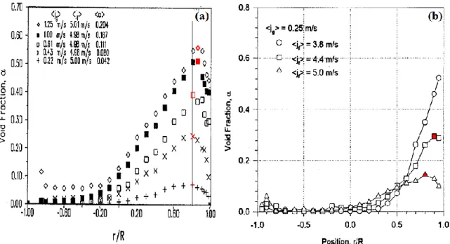
Figure 4.1 - Representation of the test conditions for dispersed bubbly flows on the flow regime map74 Figure 4.2 - Void fraction profiles, (a) constant JL (Kocamustafaogullari et al., 1994) and (b) constant JG (Iskandrani & Kojasoy, 2001) ...76
Figure 4.3 - Void fraction profiles of the METERO experiment for dispersed bubbly flows at 40D ....76
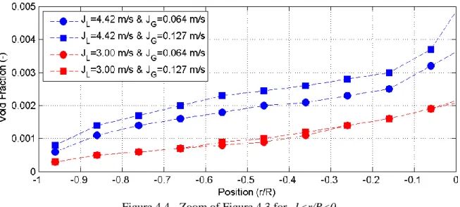
Figure 4.4 - Zoom of Figure 4.3 for -1<r/R<0 ...77
Figure 4.5 - Probability density function of chord lengths measured at 40 D for JL=4.42 m/s and JG=0.064 m/s ...77
Figure 4.6 - Chord length distribution profiles of the METERO experiment for dispersed bubbly flows at 40D ...79
Figure 4.7 -Interfacial area profiles of the METERO experiment for dispersed bubbly flows at 40D ..80
Figure 4.8 - Zoom of Figure 4.7 for -1<r/R<0 ...80
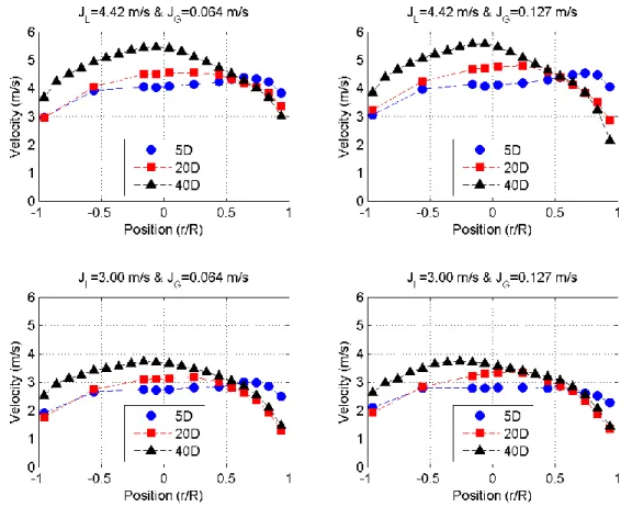
Figure 4.9 - Axial bubble velocity for various JG at the center of the test section and 40D ...82
Figure 4.10 - Axial bubble velocity for JL=4.42 m/s and various JG at the center of the test section and 40D ...82
Figure 4.11 - Axial mean velocity profiles of the METERO experiment for dispersed bubbly flows at 40D ...83
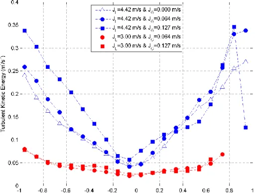
Figure 4.12 - Turbulent kinetic energy profiles of the METERO experiment for dispersed bubbly flows at 40D ...84
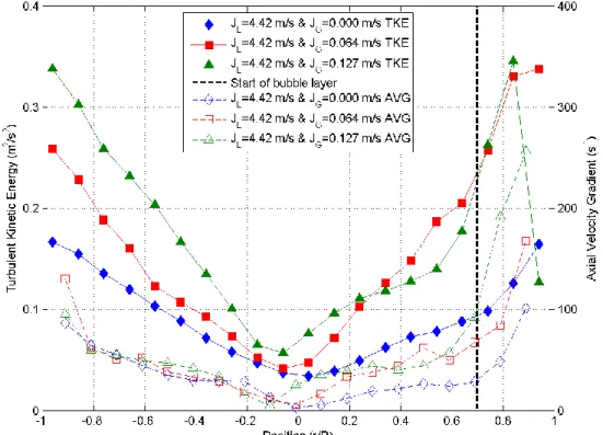
Figure 4.13 - Turbulent kinetic energy and axial velocity gradient profiles at 40D for JL=4.42 m/s and various JG ...85
Figure 4.14 - Axial evolution of void fraction profiles for dispersed bubbly flows ...86
Figure 4.15 - Axial evolution of chord length profiles for dispersed bubbly flows ...87
Figure 4.16 - Axial evolution of interfacial area profiles for dispersed bubbly flows at constant JL ...88
Figure 4.17 - Axial evolution of interfacial area profiles acquired at 0<r/R<1 for dispersed bubbly flows at constant JG ...88
Figure 4.18 - Axial evolution of axial mean bubble velocity profiles for dispersed bubbly flows ...89
Figure 4.19 - Axial evolution of axial mean liquid velocity profiles for dispersed bubbly flows ...90
Figure 4.20 - Axial evolution of turbulent kinetic energy profiles for dispersed bubbly flows ...91
Figure 5.1 - Representation of the test conditions for intermittent flows on the flow regime map ...95
Figure 5.2 - Local void fraction distributions measured at 253D for JL=1.65 m/s & JG=0.55, 1.1 and 2.2 m/s (Lewis et al., 2002) ...96
Figure 5.3 - Void fraction distribution measured at 253D for JL=1.65 m/s and various JG (Riznic & Kojasoy, 1997) ...96
5
Figure 5.4 - Void fraction profiles of the METERO experiment for intermittent flows at 40D ...97
Figure 5.5 - Zoom of Figure 5.4 for -1<r/R<0.5 ...97
Figure 5.6 - Chord length profiles of the METERO experiment for intermittent flows at 40D ...98
Figure 5.7 - Interfacial area concentration distribution measured at 253D for JL=1.65 m/s and JG=1.10 m/s (Riznic & Kojasoy, 1997) ...99
Figure 5.8 - Interfacial area profiles of the METERO experiment for intermittent flows at 40D ...100
Figure 5.9 - Zoom of Figure 5.8 for -1<r/R<1 ...100
Figure 5.10 - A typical liquid velocity profile development in liquid layer below the gas slug (Sharma et al., 1998) ...101
Figure 5.11 - Local axial mean velocity distributions measured at 253D for JL=1.65 m/s & JG=0.55, 1.10 and 2.20 m/s (Lewis et al., 2002) ...102
Figure 5.12 - Axial mean velocity profiles of the METERO experiment for intermittent flows at 40D ...102
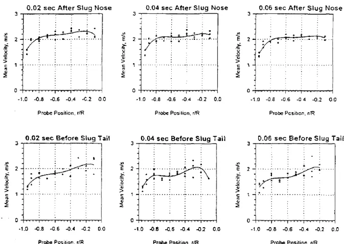
Figure 5.13 - Velocity profiles in liquid slugs (Taitel & Barnea, 1990) ...103
Figure 5.14 - Turbulent kinetic energy profiles of the METERO experiment for intermittent flows at 40D ...104
Figure 5.15 - Axial evolution of void fraction profiles for intermittent flows ...105
Figure 5.16 - Linear-linear representation of void fraction profile evolutions for JL=1.59 m/s ...105
Figure 5.17 - Passage of a slug for JL=1.59 m/s and JG=0.127 m/s at axial locations 20D (a) and 40D (b) ...106
Figure 5.18 - Axial evolution of chord length profiles for intermittent flows ...107
Figure 5.19 - Bubble layer between two slugs observed at 20D for JL=1.59 m/s and JG=0.127 m/s ...107
Figure 5.20 - Axial evolution of interfacial area profiles for intermittent flows ...108
Figure 5.21 - Axial evolution of axial mean bubble velocity profiles for intermittent flows ...109
Figure 5.22 - Axial evolution of axial mean liquid velocity profiles for intermittent flows ...109
Figure 5.23 - Axial evolution of turbulent kinetic energy profiles for intermittent flows ...110
Figure 6.1 - Generalized flow regime map for horizontal two-phase flow (Taitel & Dukler (1976) and Dukler & Taitel (1986)) ...115
Figure 6.2 - Collapsed liquid height diagram ...117
Figure 6.3 - Dimensionless flow regime map of the METERO experiment at 40D ...117
Figure 6.4 - Terminal velocity of air bubbles in liquid (water) at rest as a function of bubble size (Haberman & Morton, 1953) ...119
Figure 6.5 - The evolution of <u'> with various liquid and gas superficial velocities ...120
Figure 6.6 - Sketch of expected flow regime map ...121
Figure 6.7 - A novel dimensionless flow regime map at 40D ...123
Figure 8.1 - Representation of stratified bubbly flow with two different fluids ...131
Figure 8.2 - Observation of pulsations in plug flow with high speed camera ...131
Figure 8.3 - Detection of the boundary between bubble layer and liquid phase in plug flow ...132
Figure A2.1 - Schematic of fluid velocity with projection on the wire axes ...140
Figure A2.2 - Schematic of effective velocities and their projections on the axes of wires/films ...141
Figure A3.1 - Schematic of the areas in the test section ...142
Figure A3.2 - Schematic of the discretization in horizontal layers ...143
Figure A3.3 - Schematic of semi-crown decomposition ...144
Figure A4.1 - Displaying the bubble size with an improved method in ISO ...145
Figure A4.2 - Illustration of the intercept/diameter conversion ...146
Figure A4.3 - Representation of the averaging methods based on the measurements of Andreussi et al. (1999) ...147
6 Figure A4.5 - Study of statistical convergence for the conical probe: plot of the standard deviation of
the voltage fluctuations depending on the number of samples (Bottin, 2010) ...149
Figure A4.6 - Plot of ei 2 =f(Ueffi n ) and determination of the calibration constants for a two-component probe (Bottin, 2010) ...149
Figure A4.7 - Plot of Uaxe measured by Pitot tube as a function of Vdeb (Bottin, 2010) ...150
Figure A5.1 - Void fraction profiles measured at 40 diameters for dispersed bubbly flows ...151
Figure A5.2 - Chord length profiles measured at 40 diameters for dispersed bubbly flows ...151
Figure A5.3 - Interfacial area profiles measured at 40 diameters for dispersed bubbly flows ...152
Figure A5.4 - Axial mean bubble velocity profiles measured at 40 diameters for dispersed bubbly flows ...152
Figure A5.5 - Axial mean liquid velocity profiles measured at 40 diameters ...153
Figure A5.6 - Turbulent kinetic energy profiles measured at 40 diameters for dispersed bubbly flows ...153
Figure A5.7 - Axial evolution of void fraction for dispersed bubbly flows ...154
Figure A5.8 - Axial evolution of chord length for dispersed bubbly flows ...155
Figure A5.9 - Axial evolution of interfacial area for dispersed bubbly flows ...156
Figure A5.10 - Axial evolution of mean bubble velocity for dispersed bubbly flows ...157
Figure A5.11 - Axial evolution of mean liquid velocity ...158
Figure A5.12 - Axial evolution of turbulent kinetic energy for dispersed bubbly flows ...158
Figure A6.1 - Void fraction profiles measured at 40 diameters for intermittent flows ...159
Figure A6.2 - Chord length profiles measured at 40 diameters for intermittent flows...159
Figure A6.3 - Interfacial area profiles measured at 40 diameters for intermittent flows ...160
Figure A6.4 - Axial mean bubble velocity profiles measured at 40 diameters for intermittent flows .160 Figure A6.5 - Axial mean liquid velocity profiles measured at 40 diameters for intermittent flows ...161
Figure A6.6 - Turbulent kinetic energy profiles measured at 40 diameters for intermittent flows ...161
Figure A6.7 - Axial evolution of void fraction for intermittent flows ...162
Figure A6.8 - Axial evolution of chord length for intermittent flows ...163
Figure A6.9 - Axial evolution of interfacial area for intermittent flows ...164
Figure A6.10 - Axial evolution of mean bubble velocity for intermittent flows ...165
Figure A6.11 - Axial evolution of mean liquid velocity for intermittent flows ...166
Figure A6.12 - Axial evolution of turbulent kinetic energy ...167
Figure R.1 - La phase accidentelle dans une centrale nucléaire ...171
Figure R.2 - Les profils des grandeurs caractéristiques d’écoulement en écoulements dispersés : (a) Taux de vide (Kocamustafaogullari et al, 1994), (b) la concentration d’aire interfaciale (Kocamustafaogullari et al, 1994), (c) la vitesse axiale moyenne du liquide (Iskandrani & Kojasoy, 2001) ...172
Figure R.3 - Les profils des grandeurs caractéristiques d’écoulement en écoulements intermittent : (a) Taux de vide (Lewis et al, 2002), (b) la concentration d’aire interfaciale (Riznic & Kojasoy, 1997), (c) la vitesse axiale moyenne du liquide (Lewis et al, 2002) ...173
Figure R.4 - Installation METERO ...173
Figure R.5 - Position de mesure axiaux ...174
Figure R.6 - La sonde croisée connectée au système d'anémométrie ...174
Figure R.7 - La chute de la tension lors du passage des bulles ...174
Figure R.8 - Les détails du processus de discrimination des phases ...175
Figure R.9 - Schéma d'une quadri-sonde optique ...176
Figure R.10 - La géométrie de la quadri-sonde optique ...176
Figure R.11 - Schématique de la technique d'ombroscopie ...177
7 Figure R.13 - Vitesse axiale des bulles pour JL=4.42 m/s et de divers JG au centre de la section d'essai
et à 40D ...177
Figure R.14 - L'interaction d'une bulle sphérique avec une bi-sonde optique ...178
Figure R.15 - La carte de régimes d'écoulements pour l'installation METERO ...178
Figure R.16 - Les profils de la vitesse axiale moyenne (a) et de l’énergie cinétique turbulente (b) de la phase liquide mesurés en écoulement dispersé à 40D ...179
Figure R.17 - Les profils du taux de vide (a), de la concentration d’aire interfaciale (b) et de longueur de cordes (c) mesurés à 40D pour divers JL et JG fixé ...180
Figure R.18 - Les profils du taux de vide (a), de longueur de cordes (b) et de la concentration d’aire interfaciale (c) mesurés à 40D pour divers JG et JL fixé ...181
Figure R.19 - Les évolutions axiales du taux de vide (a), de la concentration d'aire interfaciale (b) et de longueur de cordes (c) en écoulements dispersés ...182
Figure R.20 - Les évolutions axiales des vitesses des bulles (a) et du liquide (b) ...182
Figure R.21 - Les profils des vitesses des bulles et du liquide à 40D ...183
Figure R.22 - La comparaison de l'énergie cinétique turbulente ...183
Figure R.23 - Une bulle allongée observée à l'aide de la vidéo rapide en écoulement intermittent ...184
Figure R.24 - Les profils du taux de vide (a), de la concentration d'aire interfaciale (b) et de longueur de cordes (c) mesurés à 40D en écoulement intermittent ...185
Figure R.25 - Les vitesses des bulles et de la phase liquide mesurées à 40 diamètres pour différents conditions d’essai ...185
Figure R.26 - La comparaison des vitesses axiales du liquide en écoulement disperse (bleu) et en écoulement intermittent (vert) a 40D...186
Figure R.27 - Les profils de la vitesse du liquide en écoulement intermittent (Taitel & Barnea, 1990) ...186
Figure R.28 - Les évolutions axiales du taux de vide (a), de la concentration d'aire interfaciale (b) et de longueur de cordes (c) en écoulements intermittent ...187
Figure R.29 - Changement de la taille des bulles entrée 20D et 40D en écoulement intermittent ...187
Figure R.30 - Les évolutions axiales de la vitesse (a) et l'énergie cinétique turbulente (b) en écoulement intermittent ...188
Figure R.31 - La carte de régime d’écoulement généralisée pour les écoulements diphasiques horizontaux ...188
Figure R.32 - La carte X-T pour l'expérience METERO ...190
Figure R.33 - La carte mécaniste de régime d’écoulement ...192
8
NOMENCLATURE
Latin letters
A~ Dimensionless flow cross-section (-)
G
A~ Dimensionless flow cross-section of gas phase (-)
i
A Interfacial area concentration (m-1)
k
A Area of horizontal layers (m2)
L
A~ Dimensionless flow cross-section of liquid phase (-) T
A Total cross-sectional area (m2)
wire
A Area of wire (m2)
CT Transition criteria (-)
D Internal diameter of the test section (m)
32
d Sauter mean diameter (m)
i
d0
Distance between probe tips (m)
L
D~ Dimensionless hydraulic diameter (-)
pq
d Average diameter at the moments p and q
i
t0
Time lag (time-of-flight) between probe tips (s)
wire
d Diameter of wire (m)
e Voltage across film/wire (V)
wire
E Energy stored on wire (J)
h~ Dimensionless liquid height (-)
lhC Chord length distribution function (-)
Convection
h Heat transfer coefficient / Newton convection coefficient (W/(m2.K))
lhD Bubble diameter distribution function (-)
Liq
h Liquid height (m)
lhL Distribution function (-)
I Current passing through film/wire (A)
G L J
J , Superficial velocity of liquid and gas phases (m/s)
K Turbulent kinetic energy (m2/s2)
l Length (m)
wire
l Length of wire (m)
N Correction coefficient for turbulent kinetic energy (-)
b
N Number of bubbles (-)
Nu Nusselt number (-)
Joule
P Power due to Joule effect (W)
Pr Prandtl number (-)
o w
q Heat transferred from wire to outside (J)
r
Radial position in the test section (m)R Internal radius of the test section (m)
Re Reynolds number (-)
film
Re Reynolds number of film (-)
wire
9
i
S~ Dimensionless perimeter of liquid-gas interface (-)
L
S~ Dimensionless perimeter of liquid phase (-)
p
S The moment of p order (-)
T Dimensionless dispersed bubble flow parameter (-)
a
T Ambient temperature (°C)
Gas
t Total time of gas phase presence (s)
ref
T Reference temperature (°C)
Total
t Total acquisition time (s)
wire
T Temperature of film/wire (°C)
u Fluctuating component of axial liquid velocity (m/s)
'
,
'
,
'
v
w
u
Standard deviation of fluctuating component of axial, radial and orthoradial liquid velocity (m/s)axe
U Maximum average axial liquid velocity (m/s)
B
U Bubble velocity (m/s)
eff
U Effective cooling velocity (m/s)
L
U Average Axial component of liquid velocity (m/s)
L
U~ Dimensionless axial liquid velocity (-)
inst L
U Instantaneous axial liquid velocity (m/s)
GS
LS u
u , Superficial velocity of liquid and gas phases (m/s)
U Friction velocity (m/s)
deb
V Axial average liquid superficial velocity (m/s)
Gas
V Velocity of gas phase (m/s)
L
V Radial component of liquid velocity (m/s)
liq
V Velocity of liquid phase (m/s)
X Lockhart-Martinelli parameter (-)
Greek letters
Void fraction (-)
Inclination angle (°)
Slope factor of hot-film anemometry probes (-) Thermal conduction coefficient of water (W/(m.K))
G
L
, Density of liquid and gas (kg/m3)
Surface tension (mN/m)
Kinematic viscosity (m2/s)Remarks:
Spatial averaging operator: The spatial value of variable f is written as <f> (averaging
methods are described in Appendix 3)
Graphical representation: Unless it is stated, r/R=0 represents the center of the pipe
and r/R=1 & r/R=-1 represent the upper and lower walls respectively.
11
CHAPTER 1
13
1 INTRODUCTION
The aim of this thesis work is to study horizontal flow regimes and their evolution. There are two main reasons of this work: new experimental technics are now mature to profoundly the physical mechanisms involved in the evolution of these flows and numerical tools used in safety studies should be improved continuously.
The two-phase flow simulation tool, CATHARE, used in the nuclear industry for the safety of nuclear power plants, has been improved by the French Alternative Energies and Atomic Energy Commission (CEA). In the frame of the NEPTUNE project (collaboration of EDF, CEA, AREVA-NP and IRSN), the physical models of this code are validated thanks to various experimental works such as those performed on METERO.
This experimental setup is devoted to the study of horizontal two-phase flows and their axial evolution. As explained further, the knowledge of horizontal flow regimes can be critical for the calculation of an accidental situation such as a break on the horizontal leg of the primary circuit. Although such flows have already been studied and modeled, it is important to measure previously inaccessible physical quantities that play an important role in the evolution of flow regimes by the help of new experimental technics and local probes. The evolution of a bubbly flow toward a stratified one depends strongly on two main forces acting on liquid and gas phases: turbulence, which is responsible for the break-up and dispersion of bubbles, and buoyancy, which results in the rise of bubbles toward the top of the pipe where they can coalesce eventually until phase separation is reached. Even though these forces cannot be measured directly, their consequences on the flow can be.
The research efforts on this topic should focus on the following areas:
Comprehension and explanation of the physical mechanisms which drive flow regime
transitions in horizontal pipe. Although the studies in the literature bring fundamental results
for horizontal flows and the study of Bottin (2010) has introduced some detailed results in dispersed bubbly flows in horizontal pipe, it is necessary to gather more data and understand the flow regimes (increase the spatial resolution of measurements for various flow rates, etc.). For this reason, some questions should be answered such as:
o “What is the spatial distribution of the phases?”
o “Does coalescence or break-up of bubbles take place in flows?” o “What are the effects of liquid and gas flow rates?”
o “What is the nature of the interactions between liquid and gas phases?”
o “How could the competition between turbulent and buoyancy forces be described?” o “Is it possible to obtain a simple and natural flow regime transition indicator which
can be used in the simulation tools and industrial codes?”
Description, analysis and modeling of the axial development of horizontal two-phase flow
focusing particularly on the evolution of the interfacial area concentration and the turbulent kinetic energy. Two-phase flows occurring in a hot/cold leg of a nuclear reactor are
developing flows since their lengths are in the order of few diameters. Analyzing and modeling of these flows and their transitions is one challenge in multiphase research and development (R&D). Although, the industrial case points out developing two-phase flows in the pipes, the studies in the literature were focused on developed two-phase flows which are established at great distances from the entrance (lengths in the order of 200-300 diameters).
14 In the light of this information, turbulent and buoyancy forces can be considered as the two main phenomena whose competition determine the horizontal two-phase flow regime. For better understanding of two-phase flow and better modeling, particular attention should be paid to the interfacial area concentration (the area of the bubble surfaces per unit volume) and turbulent kinetic energy in the flows. There are two main reasons why the interfacial area concentration is one of the quantities of interest. Firstly, the interfacial area is involved explicitly in many interfacial exchange models (phase change, friction between phases). Secondly, its order of magnitude is an indicator of flow regimes (low in stratified flows and high in dispersed bubbly flows). Concurrently, turbulence has an important role in two-phase flow regime transitions by mixing the phases and leading to break-up of the bubbles in the flow. As a result, the turbulent kinetic energy is a quantity that can help to characterize the flow regime.
1.1 Industrial Context
Two-phase flows occur in many industrial sectors such as chemistry, petroleum, automotive, nuclear, etc. In the nuclear sector context, most of the studied hypothetical accidents are the consequence of a break on a pipe of the primary circuit leading to a loss of water. Since the water in this circuit is at high pressure (150 bar) and temperature (300 °C), the depressurization of water results in important vaporization. Thus, two-phase flow appears near the break and propagates in the entire circuit and in the reactor core.
Safety criteria concerning the temperature evolution of fuel clad depend on the remaining water mass inside the core and on what appends in all the circuit during the generation of two-phase flow. The ratio of liquid to steam flowing out at the break determines the evolution of the accident. When it is high, the pressure decreases slowly which is disadvantageous since the safety injections are automatically activated at medium pressure. In addition, core mass inventory decreases rapidly. On the other hand, for a low value of this ratio, pressure decreases rapidly and the liquid mass decreases slowly. Consequently, great amount of core energy is evacuated via steam enthalpy and this is a favorable situation in the nuclear safety. The ratio of liquid to steam near the break is determined by the local flow regime. As an example, the quantity of liquid flowing at a pressurizer discharge valve (TMI accident, 1979) (see Figure 1.1) depends on the flow regime at the junction between the hot leg and the pressurizer (see Figure 1.2): in case of stratified flow, the flowing fluid will be essentially steam while it will be essentially water in case of bubbly flow.
Figure 1.1 - Accidental situation due to loss of coolant at pressurizer Pressurizer discharge
15 Figure 1.2 - Illustration of the importance of bubble-stratified transition to predict correctly the mass
and energy lost in a break or discharge valve of the pressurizer
In this context of the improvement of safety numerical tools, the NEPTUNE project was initiated by CEA, EDF, AREVA-NP and IRSN at the end of 2001. The purposes of this project are to build a new software platform for advanced two-phase flow thermal-hydraulics allowing easy multi-scale and multi-disciplinary calculations and develop new physical models and numerical methods for each simulation scale as well as their coupling in order to meet the industrial needs. As a result, the NEPTUNE research program covers all levels of modeling (from the nucleation scale to the reactor scale) and focuses on different areas as software development, modeling and experimental studies.
In order to study, understand and model occurrence of stratification in horizontal two-phase flows, METERO (Maquette d’Etude des Transitions d’Ecoulements air/eau) has been designed as a part of the NEPTUNE project.
The experimental results obtained in the METERO experiment will support the validation and improvement of the existing models in the CATHARE code. The current industrial version of the code, CATHARE 2, is based on the two-fluid model with 2x3 equations: balance of mass, momentum and energy for liquid and gas phases. Thanks to the recent measurement technics that give access to physical quantities playing an important role in the flow evolution such as turbulent kinetic energy or interfacial area; it makes sense to add new equations for the transport of these quantities since direct validation is now possible. Therefore, a new version of the code, CATHARE 3, is under development. This new version includes a multi-field approach (splitting of the liquid phase into film and droplet fields that behave separately), transport equations for interfacial area concentration and turbulent kinetic energy. Moreover, the simplified flow map used in CATHARE 2 (as well as those found in the literature) is based on developed flows while it is never the case in nuclear power circuits. Thus, results of the METERO experiment allow checking if developed flow models have to be corrected or not for developing flows.
1.2 State of Art
Two-phase air/water flows have been investigated in the light of measured typical flow parameters such as void fraction, bubble size, interfacial area, velocity and turbulent quantities. In the literature, there exist many publications about vertical two-phase flows; however, the studies about horizontal flows are very limited compared to the studies on vertical flows.
The quantities concerning horizontal two-phase flow (dispersed bubbly and intermittent flows) have been measured and modeled by a few authors in the literature.
Kocamustafaogullari & Wang (1991) presented local distributions of void fraction, interfacial area concentration, mean bubble diameter, bubble interface velocity, chord-length (intercept length) and bubble frequency in horizontal air-water bubbly flow. The authors measured local quantities in a transparent circular pipe line which has a 50.3 mm internal diameter and is 15.4 m in length. In their
16 measurements, a double-sensor resistivity probe was used with a sampling frequency of 20 kHz and sampling time of 1s. Concerning the test conditions, the water superficial velocity ranged from 3.74 to 5.71 m/s while the air superficial velocity varied from 0.25 to 1.37 m/s. In addition, the range of average void fraction was from 0.043 to 0.225 during the tests. The experimental results showed that void fraction, interfacial area and bubble frequency values increase by decreasing the liquid flow at constant gas flow or increasing gas flow at fixed liquid flow. In addition, local maxima near upper wall have been observed in the distribution profiles of these flow quantities. The bubble interface velocity has a relatively uniform distribution except near upper wall where a sharp decrease of velocity was observed. Furthermore, the authors stated that the average interface velocity and turbulent fluctuations are increasing with an increase in the gas flow. Mean bubble diameter was calculated by using the relationship between void fraction, interfacial area concentration and mean bubble diameter. It was observed that the mean bubble diameter generally increases with an increase in gas flow rate at fixed liquid flow rate; however, this effect is not significant. In conclusion, the effects of inlet and boundary conditions on the distribution of local flow quantities (void fraction, interfacial area, etc.) were investigated in this study. Moreover, the authors recommended that further studies are essential to understand the effects of inlet conditions and wall on the distribution of the flow quantities in horizontal flows.
Similar to the study mentioned above, Kocamustafaogullari et al. (1994) studied local distributions of void fraction, interfacial area concentration and Sauter mean diameter in air-water horizontal bubbly flows. In addition, area averaged values of these flow quantities were also investigated in this study. The measurements have been performed on an experimental setup which consists of a transparent circular pipe with 50.3 mm internal diameter and is 15.4 m in length. In addition, water was circulated in a closed loop and air is circulated in an open loop in which the air was released to the atmosphere at the outlet of the test section. The local flow quantities have been acquired at 253 diameters downstream of the air-water mixing chamber by using double-sensor resistivity probe for various test conditions such as liquid superficial velocity ranging from 3.74 to 6.59 m/s, gas superficial velocity ranging from 0.21 to 1.34 m/s and average void fraction ranging from 0.037 to 0.214. The results showed that the inlet conditions have significant effects on the local and area-averaged values of the flow quantities. Decrease in liquid flow rate for constant gas flow or increase in gas flow rate for fixed liquid flow rate results in an increase in the local and area-averaged values of void fraction and interfacial area concentration. Moreover, the effect of liquid flow on these values is not as significant as that of gas flow. On the other hand, change in liquid flow has more significant effect on Sauter mean diameter values compared to effect of gas flow. Furthermore, area averaged interfacial area concentration values have been compared with those calculated by using different models existing in the literature for vertical flows. This comparison showed that the models for the vertical flows are not applicable for the horizontal flows. Thus, the authors introduced new mathematical models based on mechanistic modeling of the bubble break-up process to predict the area averaged values of interfacial area concentration and Sauter mean diameter for horizontal flows by using. The predicted values by the models were in good agreement with ones measured by a double-sensor resistivity probe.
Lewis et al. (1996) published their study about time averaged local values of void fraction due to small and large bubbles, mean liquid velocity and liquid turbulence fluctuations in horizontal air-water slug flow. The measurements have been performed on a circular transparent pipe (50.3 mm internal diameter, 15.4 m in length) by using hot-film anemometry and conical shaped (TSI 1231-W) hot-film probes which were located 253 diameters downstream of the inlet. The tests have been carried out for various liquid and gas superficial velocities (range from 1.10 to 2.20 m/s for water and range from 0.27 to 2.20 m/s for gas) at an operating temperature about 20-22 °C. The void fraction profiles
17 showed that the void fraction due to large bubbles decreases toward the upper wall while total void fraction increases slightly in this part. This slight increase indicates the contribution of small bubbles to the total void fraction due to the strong migration of small bubbles to the upper part of the pipe. In addition, either decreasing water flow rate for fixed gas flow rate or increasing gas flow rate for a given liquid flow rate results in an increase in the void fraction. Furthermore, it was observed that the liquid velocity distribution is asymmetrical and the degree of asymmetry increases with a decrease in liquid flow rate or an increase in gas flow rate. In addition, the velocity profile results show that there exists a strong shear layer starting at the top of the bottom liquid layer. In addition, velocity profiles similar to the ones observed at a fully developed turbulent pipe flows have been acquired at the bottom liquid layer and the top portion of liquid slug. The effect of inlet conditions on turbulence, namely flow rates, has been clearly seen in the results. An increase in liquid and/or gas flow rates results in an increase of both the absolute value of turbulence and the turbulence intensity. In addition, the effects of flow rates are greater within the liquid slug. The authors concluded that their results are a starting point to understand the horizontal intermittent two-phase flow and additional data is essential to understand these flows in details. Moreover, time averaged results limits to study structures of liquid slugs and the liquid layer below the gas slugs separately. Thus, instantaneous velocity measurements are necessary.
Riznic & Kojasoy (1997) have investigated local interfacial area concentration, void fraction, interfacial velocity and slug bubble frequency in horizontal air-water slug flows. The tests were carried out on a transparent circular pipe which has 50.3 mm internal diameter and is 15.4 m in length. In addition, slug flows were generated with various liquid and gas superficial velocities (ranging from 0.55 to 2.20 m/s for water and from 0.27 to 2.20 m/s for air) and void fraction between 0.1 to 0.7. The measurements were performed at an axial location of 253 diameters downstream of inlet by using four-sensor resistivity probe (for instantaneous phase velocity and interfacial concentration area due to large air slug bubbles) and two-sensor resistivity probe (for interfacial area concentration due to small bubbles). The interested quantities, except the slug bubble frequency, were measured not only at radial profiles (two-dimensional representation) but also across the pipe cross section (three-dimensional representation). Void fraction results show that void fraction increase while decreasing the liquid flow rate or increasing the gas flow rate. The authors stated that the total interfacial area concentration measured in slug flows is determined by the air slug and small bubbles. Void fraction and interfacial area concentration profiles showed that these flow quantities are distributed asymmetrically indicating non-symmetrical transport in a horizontal intermittent two-phase flow. Furthermore, slug frequency results indicate the effects of inlet conditions such that increasing liquid flow rate raises the slug frequency. On the other hand, slug frequency has a different trend with an increase in gas flow rate: it first increases and then decreases. The authors concluded that more detailed study is essential to understand the influence of inlet conditions on the slug frequency.
Bertola (2002) has studied the slug velocity and gas-liquid interface velocities for horizontal air-water two phase flows in a 12-meter-long circular transparent pipe with 80 mm internal diameter. Air-water two-phase flows were generated for liquid superficial velocities ranging from 0.6 to 2 m/s and gas superficial velocities ranging from 0.3 to 8 m/s at atmospheric pressure and temperature. The acquisitions were performed at axial locations of 96, 101 and 104 diameters from the inlet of pipe. In this study, gas-liquid interface velocities were calculating by cross-correlating phase density function time series obtained by a pair of single-fiber optical probes. The duration of the acquisitions is 400 seconds with a sampling frequency of 2 kHz. Slug velocities acquired in the tests have been compared to the slug velocities calculated by a model introduced by Dukler & Fabre (1994). This comparison showed that the model can predict the slug velocity for the mixture flows which have a Froude number
18 smaller than 3.5. For the flows with greater Froude number, the model overestimates the slug velocity. Thus, it is essential to introduce a different slug velocity correlation for these flows.
Iskandrani & Kojasoy (2001) presented their experimental results in terms of time averaged local values of void fraction, bubble-passing frequency, axial mean liquid velocity and the liquid turbulence fluctuations in horizontal air-water bubbly flows. These flow quantities were measured, in a transparent circular pipe (50.3 mm internal diameter and 15.4 m in length) by using a conical shape (TSI 1231-W) hot-film probes located at 253 diameters downstream with constant temperature anemometry system. The test were performed with various liquid and gas superficial velocities (from 3.8 to 5.0 m/s for water and from 0.25 to 0.8 m/s for air) at atmospheric pressure and temperature about 20-22 °C. Void fraction and bubble-passing frequency results showed that the profiles of both flow quantities have local maxima near the upper wall. In addition, the profiles become more flat when the liquid flow rate is increased. An increase of gas flow rate at fixed liquid flow rate also affects the flow quantities such that both void fraction and bubble passing frequency are increased. Axial mean liquid velocity is distributed uniformly except near the upper pipe wall where a sharp decrease in velocity is observed. Increasing gas flow rate results in an increase in mean velocity and turbulent fluctuations. Furthermore, the turbulent intensity at very low void fractions is slightly lower than the one in single phase flows. In addition, the turbulent intensity is increased with respect to an increase in the void fraction. Thus, the authors concluded that the local turbulence intensity is mainly a function of the local void fraction.
Yang et al. (2004) presented their study about turbulent structure in horizontal air-water bubbly flow. The turbulence structure was measured by using two X type (1246-60W) hot-film probes operated with an over heat ratio of 1.08. In addition, the measurements were taken in 1s with a sampling frequency 20 kHz. The probes were installed at 172 diameters downstream and on a horizontal transparent tube (10 m in length) with a 35 mm internal diameter. Horizontal bubbly flows were generated liquid and gas superficial velocities ranged from 3.5 to 4.5 m/s and from 0.00 to 0.44 m/s respectively. The operating pressure is 214-319 kPa and the working temperature is about 28 °C. The experimental results showed that mean axial liquid velocity, turbulent fluctuations and turbulent intensity have asymmetric distributions at measuring angles 0° and 45°. On the other hand, they are symmetric when the measuring angle is 90°. In the lower part of the tube, the mean axial liquid velocity profiles have a similar trend of what is observed in single phase flows. In the upper part where the bubbles are accumulated, the velocity decreases sharply. By increasing gas flow rate, mean velocity increases in the lower part. On the other hand, a decrease in mean velocity in the upper part was observed for the same condition. In the lower part, the turbulence structure is similar to that observed in fully developed single phase flows. The turbulence increases in the upper portion and reaches a maximum point. After this maximum, it decreases in the region near upper tube wall. The authors concluded that there is a strong momentum exchange in the circumferential direction that may be induced by the bubble immigration. In our point of view, the experimental results of Yang et al. (2004) are significantly contributive to the error calculation of spatial averaging methods for turbulent kinetic energy since the turbulence structure was measured in three different angles.
As a general trend in literature, flow regime maps are generated by the help of the visual observations. However, these maps could not represent the flow regime transitions universally due to the dependence of experimental facility conditions and properties. In addition, the lack of precision in describing these visual observations brings problems to the classification of flow regimes and their transitions. At this point, Taitel & Dukler (1976) introduced a mechanistic model which predicts the relationship between operation conditions (gas and liquid flow rates, properties of fluids, pipe diameter and angle of inclination) and flow regime transitions in horizontal and near horizontal flows. This
19 model is based on physical concepts and it is very successful to predict flow regimes and transitions. By using this model, the authors created a generalized dimensionless flow regime map for horizontal flows. This flow regime map was in a good agreement with the experimental data collected from the literature. The model and the flow regime map introduced by the authors motivate us to generate a dimensionless flow regime map for the METERO experiment and to develop analytical criteria for flow regime transitions.
Ekambara et al. (2008) presented a CFD simulation study on the internal phase distribution of co-current, air-water bubbly flow in a horizontal pipeline which has a 50.3 mm internal diameter. Liquid and gas superficial velocities varied from 3.8 to 5.1 m/s and from 0.2 to 1.0 m/s respectively. In addition, average void fraction was ranging from 0.04 to 0.16. The results of the predicted void fraction and the mean liquid velocity were compared to the experimental data taken from the literature. There exists a good agreement between the predicted and experimental results. In the study of Ekambara et al. (2008), it is more delightful to note that horizontal gas-liquid two phase flows were classified with respect to the dominant mechanism in the flows. The authors organized the flows in three groups: gas dominant, liquid dominant and gas-liquid coordinated. In gas dominant flows, the flow is controlled by gas phase and the liquid phase exists in droplets (for instance, mist flow). If the liquid flow rate reaches a certain level where the flow is driven by liquid phase, this flow is called liquid dominant flow. Dispersed bubbly flow is a representative example of liquid dominant flows. In the case of gas-liquid coordinated flows, neither gas phase nor liquid phase can control the flow. Buoyant bubbly, plug, slug and wave flows are in this group. This flow regime classes have already been used in the METERO experiment to define the generated flow regimes.
Bottin (2010) presented a PhD thesis which was focused on local distribution and axial evolution of flow quantities in horizontal single phase and two-phase flows (void fraction, bubble size, interfacial area, velocities of liquid and gas phases and turbulence) and modeling of turbulence and interfacial area in horizontal dispersed bubbly flows. The author performed tests in the METERO experiment (details will be given in Chapter 2) at three different axial locations: 5, 20 and 40 diameters downstream of the inlet. Furthermore, as a part of the thesis, the author defined flow regimes by the help of high speed camera visualizations and presented a flow regime map for the METERO experiment, as seen in Figure 1.8. These flow regimes were defined in 5 major groups such as Buoyant Bubbly Flow (BBF), Stratified Bubbly Flow (SBF), Plug Flow (PF), Slug Flow (SF) and Stratified Flow. The descriptions of these flow regimes are given in the following paragraphs.
Buoyant Bubbly Flow (BFF) is a flow regime where the bubbles are dispersed in liquid phase. The bubbles are not in contact with other bubbles, as seen in Figure 1.3. The bubbles are not distributed uniformly in the test section compared to fully dispersed flows since buoyancy force results in the migration of the bubbles to the upper part. The effects of non-uniform bubble distribution can be observed in the flow quantity profiles. Bottin (2010) stated that fully dispersed bubbly flows cannot be achieved in the METERO experiment since the liquid flow rates cannot reach certain values to establish full dispersion.
In Stratified Bubbly Flow (SBF), as seen in Figure 1.4, the bubbles start to accumulate at the upper part of the test section and form a mattress of bubbles. The motion of the bubble mattress is different from the liquid phase which determines the motion of the bubbles at the lower part. It can be conclude that there exist two different flows in the test section which are gas dominant at the upper part and liquid dominant at the lower part. Thus, this flow is a clear example of gas-liquid coordinated flow defined by Ekambara et al. (2008).
20 Figure 1.3 - Buoyant bubbly flow for JL=5.31 m/s and JG=0.0255 m/s (Bottin, 2010)
Figure 1.4 - Stratified bubbly flow for JL=4.42 m/s and JG=0.1273 m/s (Bottin, 2010)
Plug Flow (PF) is described such that air plugs are generated and the number of air plugs increases while decreasing liquid flow rate. As seen in Figure 1.5, there exist small bubbles in the lower part of the test section and bigger bubbles around the air plugs.
In Slug Flow (SF), slugs are generated by decreasing the liquid flow rate at a constant gas flow rate. In addition, the coalescence of the small bubbles and air plugs occur in the turbulence since turbulence, which is the main source of bubble break-up, is decreased. As a result, Taylor bubbles are observed in the upper part and small bubble take place in liquid slugs as seen in Figure 1.6.
Top View
Side View
Top View
21 In Stratified Flow, there exist two separated phases flowing parallel to each other. Although there is a velocity difference across the phase interface, it is not sufficient to establish air pockets in the flow, but the waves occur on the interface as seen in Figure 1.7.
Figure 1.5 - Plug flow for JL=2.19 m/s and JG=0.0637 m/s (Bottin, 2010)
Figure 1.6 - Slug flow for JL=0.53 m/s and JG=0.0637 m/s (Bottin, 2010)
Top View
Side View
Top View
22 Figure 1.7 - Stratified flow for JL=0.39 m/s and JG=0.0955 m/s (Bottin, 2010)
Figure 1.8 - METERO flow regime map at 40D
As mentioned before, the flow quantities were measured at three axial locations by Bottin (2010). For this purpose, X shaped hot-film probes with a constant temperature anemometry (CTA) system has been used in single phase flows. In two-phase flows, two-point optical fiber probes and conical hot-film probes with CTA have been used for the measurements. The details of these probes are given in Chapter 3.
The results of Bottin (2010) showed that the distribution of gas phase results from the competition between buoyancy force which tends to migrate bubbles to the top of the test section and turbulent force which promotes the homogenization of the phases. Thus, spatial distribution of the bubbles depends on the bubble size and flow variations. The effects of spatial distribution were observed in the radial profiles of flow quantities such as Sauter mean diameter, interfacial area concentration and void fraction. In addition, the author stated that the evolution of average interfacial area shows a linear
Top View
23 dependence as a function of gas superficial velocity. In addition, the presence of bubbles was also observed in velocity and turbulence profiles. For instance, the liquid velocity decreases sharply at the top of the pipe where the bubbles are accumulated. This velocity decreases results from the additional turbulence introduced by bubbles. Moreover, presence of bubbles brings out an asymmetrical distribution of velocity and turbulence profiles. The axial evolution of the flow quantities gives access to observe sedimentation or coalescence of bubbles. The author also presented mathematical models of average turbulent kinetic energy and interfacial area transport. The comparison of experimental results and turbulent kinetic energy model showed that the model shows a good estimation of average kinetic energy at 40 diameters; however, the estimation of axial evolution is poor. The results of the interfacial area transport model are a good agreement with the experimental results obtained for low gas flow rates. For higher flow rates, the model does not represent the physics of the flow due to the lack of data. Thus, further investigation is essential to develop the models.
As seen from the studies mentioned above, most of them, except the one of Bottin (2010), were performed to measure the flow quantities of developed flows at locations relatively far from the inlet of the test section (from 172 to 253 diameters from the inlet which are longer than the lengths in the PWRs, around 10 diameters) and the axial evolution of the flow quantities are not in the focus of these studies. The experimental study on developing dispersed bubbly and intermittent flows is necessary to model correctly the transport of interfacial area and mean turbulent kinetic energy. Thus, this study is devoted to the experimental investigation on the flow quantities of developing flows and their modeling.
1.3 Report Plan
This thesis report consists of 7 chapters and is organized as:
Chapter 1 introduces the start point of this thesis by presenting the industrial and scientific context and gives some example studies on horizontal two-phase flows from literature.
In Chapter 2, the experimental setup (METERO) is presented. Chapter 3 gives detailed information about the measurement techniques (optical fiber probes, hot-film anemometry and high-speed camera), instrumentation, acquisition and post-processing procedures (programs, routines, analysis, averaging methods and uncertainties).
In chapters 4 and 5, local and axial studies of the flow quantities (void fraction, Sauter mean diameter, interfacial area concentration, phase velocities, etc.) in dispersed bubbly and intermittent flows are presented. Chapter 6 is dedicated to dimensionless flow regime maps generated for the METERO experiment.
Chapter 7 concludes the thesis and presents the outlook that highlights the originality of the present work and contributions of this thesis.
There exist 6 appendices in this thesis. The first four appendices give detailed information about methods and techniques used in the present work. In addition, appendices 5 and 6 present all experimental results acquired in the METERO experiment during the present work.
25
CHAPTER 2
27
2 EXPERIMENTAL SETUP
2.1 Objectives and Challenges
METERO (Maquette d’Etude des Transitions d’Ecoulement air/eau) (Figure 2.1), designed in 2004 and operated first in 2006) is the first experiment of the co-developed CEA-EDF NEPTUNE project.
Figure 2.1 - The METERO experiment
As mentioned previously, the METERO experiment is dedicated to understand the responsible mechanisms of the transition between bubbly and stratified two-phase flows in a horizontal pipe. This experiment is also used to create experimental databases for thermal-hydraulics simulation code CATHARE (Code Avancé en ThermoHydraulique pour les Accidents dans les Réacteurs à Eau) and to validate 1D (size averaged) models for interfacial area concentration transport and turbulent kinetic energy in CATHARE code. This experiment may also be used to create future models for NEPTUNE CFD codes.
The METERO experiment allows measuring various two-phase air/water flow quantities, such as void fraction, interfacial area, bubble sizes, velocity of the gas phase, liquid height, turbulence level, mean and fluctuating velocity of the liquid phase, etc., in order to analyze two-phase flows in details. This chapter is devoted to describe the METERO experiment.
2.2 Description of the Experimental Setup
The schematic of the experimental setup is presented in Figure 2.2.
The air/water flow is generated in a transparent 5.4-meter-long horizontal circular pipe which is made of Plexiglas with an internal diameter of 100 mm and a wall thickness of 10 mm. In the METERO experiment, air/water two-phase flows can be generated with various air and water flow rates such as:
from 1 to 150 m3/h for water flow
28 and from 1 to 60 m3/h (or 1000 Nl1/min) for air flow (used up to 350 Nl/min due to pressure
drops).
These flow rates generate various single phase axial velocities of 0.5 to 5.31 m/s for water and 0.5 to 0.8 m/s for air. The method to obtain phasic velocities from the gas flow rates is summarized in Appendix 1.
2.2.1 Water and air circuits
The water circuit consists in: a non-pressurized water storage tank with 1500-liter-capacity supplied with city water (tap water). There exists heat exchange circuit and water level sensor inside the tank. In the beginning, the water was initially distilled through a demineralization system to prevent the contamination of water by minerals and particles that might damage the anemometer probes. The use of the demineralization system has been abandoned with the appearance of triboelectric phenomena strongly arisen with demineralization.
The temperature variations of water can significantly affect the measurements. These variations are limited to 0.1 °C and 0.5 °C for hot-film anemometry and optical fiber probe measurements respectively. Thus, the storage tank is equipped with a heat exchanger circulating industrial water to control temperature variations of the water.
A filter with 5 µm mesh size is installed on a by-pass to filter water to prevent the contamination of water by particles which may damage the probes.
a water circulation system (pump provided by Finder with 2.8 bar discharge pressure, 150 m3/h maximum flow rate and 18.5 kW electrical power) connected to the test section via two flow measurement lines:
o a line with a nominal diameter of 25 mm for 0-to-15 m3
/h range associated with a Coriolis mass-flow meter,
o a line with a nominal diameter of 100 mm for 15-to-150 m3
/h range associated with a volumetric electromagnetic flow meter.
The water is circulated in a closed circuit such that the water flows through the test section and returns to storage tank which acts as a cyclone separator at the tangential inlet. A grid system, seen in Figure 2.3, is installed in the storage tank to eliminate the bubbles in the water circuit.
1
A normoliter (Nl) represents a liter under normal conditions (temperature of 273.15 K and pressure of 101325 Pa).
29 Figure 2.2 - Schematic of the experimental setup: (1) Water storage tank, (2) pomp, by-pass and filter, (3) water flow rate measurement system, (4) air filtration and flow rate measurement system, (5) fluid
injection, (6) test section
2 1 4 5 6 Flow d ir ec tion 3