HAL Id: hal-00126253
https://hal.archives-ouvertes.fr/hal-00126253
Submitted on 24 Jan 2007
HAL is a multi-disciplinary open access
archive for the deposit and dissemination of
sci-entific research documents, whether they are
pub-lished or not. The documents may come from
teaching and research institutions in France or
abroad, or from public or private research centers.
L’archive ouverte pluridisciplinaire HAL, est
destinée au dépôt et à la diffusion de documents
scientifiques de niveau recherche, publiés ou non,
émanant des établissements d’enseignement et de
recherche français ou étrangers, des laboratoires
publics ou privés.
Experimental investigation of the fluctuation dissipation
relation in a spin glass
D. Hérisson, M. Ocio
To cite this version:
D. Hérisson, M. Ocio. Experimental investigation of the fluctuation dissipation relation in a spin
glass. SPIE Conference: Fluctuations and Noise (Noise as a Tool for Studying Materials), 2003,
United States. pp.5112, 25-37. �hal-00126253�
Experimental investigation of the fluctuation dissipation
relation in a spin glass.
Didier H´
erisson and Miguel Ocio
DSM, Service de Physique de l’ ´
Etat Condens´
e, CEA-Saclay, 91191 Gif sur Yvette Cedex,
France
ABSTRACT
We present the first experimental determination of the time auto-correlation of magnetization in the non-stationary regime of a spin glass, and its quantitative comparison with the corresponding response, the magnetic relaxation function. These measurements were performed in a new experimental setup working as an absolute thermometer. Clearly, we observe a non-linear fluctuation-dissipation relation between correlation and relaxation, i.e. an effective temperature higher than the bath temperature in the aging regime. According to theoretical developments on mean field models, and lately on short range ones, in the limit of very large waiting times, the relation between relaxation and correlation in the aging regime becomes temperature independent for a given system. A scaling procedure allows us to extrapolate to the limit of long waiting times by separating station-ary and non-stationstation-ary regimes and to check the validity of the temperature independence of the fluctuation dissipation relation in the non-stationary regime.
Keywords: Spin glass, non-stationarity, fluctuation dissipation relation.
1. INTRODUCTION
The derivation of the fluctuation dissipation theorem (FDT)1, 2which links the response function of a system to
its time autocorrelation function, represented a great progress in statistical physics since it made it possible to work out dynamics from the knowledge of statistical properties at equilibrium. Nevertheless, this progress was limited by severe restrictions. FDT applies only to ergodic systems at equilibrium. It is a direct consequence of the ergodic property that, for a given observable, time averages are equivalent to thermodynamic ensemble averages, or, physically, that the system is invariant by time translation. Yet, such systems represent a very limited part of natural objects, and there is now a growing interest on non-ergodic systems. A possible way on the challenging problem of the existence of fluctuation dissipation (FD) relations valid in off-equilibrium situations, is to extend equilibrium concepts to non-stationary systems not too far from equilibrium. Glasses are such systems; they remain strongly non-stationary even when their rate of energy decrease has reached undetectable values. In the absence of any external driving force, they slowly evolve towards equilibrium, but never reach it, even on geological times. In these systems, though two-times dependent quantities (like the response to a field perturbation) are always far from equilibrium, one-time dependent quantities (like the average energy) are near equilibrium values .
About 15 years ago, the first experiments on spontaneous “thermodynamic” magnetic fluctuations were performed on a spin glass system.3 At that time, the purpose of the experiment was to measure the so called
“1/f ” noise which could be expected in these systems with a large distribution of relaxation times. Data analysis was performed by classical FFT methods, and within the frequency range of the first experiments, it was found that the power spectrum was stable and related by FDT to the out-of-phase susceptibility.4, 5 At the same
period, the strong non-stationarity of spin glasses was experimentally detected6, 7 and related later to equivalent
properties of glassy polymers already investigated long time before.8 Very soon too, the non-stationarity of
the very low frequency magnetic noise power spectrum was detected,4 showing that the behavior of these
systems is quite different when looking on different timescales. The non-stationarity of spin glasses, the so-called “aging” was the subject of intensive experimental studies.9 Meanwhile, the theoretical community was mainly
preoccupied by the solution of the problem of the Gibbs equilibrium state. Unfortunately for experimentalists,
the only solvable model of a spin glass was the Sherrington-Kirkpatrick (SK) mean field model —which has a rather loose relation with a real spin glass—, but the output was finally the concept of hierarchical ultrametric phase space organization derived by Parisi and coworkers.10 Despite its esoteric nature, this concept was a very
powerful qualitative tool, making understandable most of the far from intuitive manifestations of non-stationarity in spin glasses, what is known now as “rejuvenation” and “memory” effects.11
2. GENERALIZED FLUCTUATION DISSIPATION RELATION
In its basic form, FDT reads
R(t − t′
) = β∂C(t − t′
)/∂t′
, (1)
where R(t, t′
) is the impulse response of an observable to its conjugate field (the impulse is applied at time t′
and measurement is done at time t), C(t′
, t) is the time autocorrelation of the observable and β = 1/kBT . Actually,
FDT is intimately linked to the thermodynamic definition of the temperature. In non-stationary systems, FDT is not expected to hold. A quite general relation can be written as
R(t′
, t) = βX(t′
, t)∂C(t′
, t)/∂t′
(2) (Note that now t and t′
are referred to the “birth” of the system, i.e. the instant where, by the variation of some control parameter —temperature, concentration— it enters in its glassy state). FDT corresponds to X = 1. Determination of X, the fluctuation dissipation ratio (FDR), or of an “effective temperature” Tef f = T /X, was the aim of many recent theoretical studies, following the seminal works of L. F. Cugliandolo
and J. Kurchan.12, 13 In mean field models, a generalization of FDT was predicted on the basis of the ”weak
ergodicity breaking” scenario.14 It was conjectured that, in the asymptotic limit of large times, when stationary
and non-stationary timescales are well separated, the FDR would depend on time only through the correlation function: X(t′
, t) = X(C(t′
, t)) for t′
(and t > t′
) → ∞. The dependence of X on C would reflect the level of thermalization within different timescales.15 The integrated form of the FD relation would become
χ(t′
, t) = β Z C(t,t)
C(t′,t)
X(C)dC (3)
(susceptibility function), and
σ(t′
, t) = β
Z C(t′,t)
0
X(C)dC (4)
(relaxation function). The equilibrium limit of χ(t′
, t) would read χeq= β Z C(t,t) 0 X(C)dC = β(1 − Z 1 0 C(X)dX) (5)
(in the simplest Ising case with C(t, t) = 1), formally equivalent to the Gibbs equilibrium susceptibility in the Parisi replica symmetry solution for the SK model,16 with C ⇔ q (overlap between pure states) and X ⇔ x (repartition of overlaps). Within PaT hypothesis,17 it was shown that in the non-stationary regime, i.e. for
C < qEA, the χ(C) curve is temperature independent, and thus unique for a given system. Theoretical works,
analytical18(with the constraint of stochastic stability) and numerical19 (with the problem of size effects) were
done in order to confirm the above properties in short range models. FDT links linearly the relaxation function σ(t′
, t) — as well as the susceptibility function χ(t′
, t) — to the autocorrelation function: for instance, σ(t′
, t) = βC(t′
, t). Non-equilibrium properties can be characterized and classified by the deviations from this relation.
3. EXPERIMENTAL BACKGROUND
3.1. Principle of measurement: an absolute thermometer
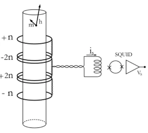
Measurement of magnetic fluctuations is conceptually a very simple experiment. The sample, of cylindrical shape, is inserted into a pick-up (PU) coil connected by a twisted pair of wires to the input coil of a SQUID (Fig. 1); the
Figure 1. Basic SQUID circuit for magnetic fluctuations measurement.
whole circuit is made of superconducting (SC) wire. The system is contained in a4He cryogenic setup allowing
temperature regulation above 4.2K. Moments fluctuations in the sample induce a fluctuating flux in the PU. From flux conservation in the SC circuit, this fluctuating flux generates a fluctuating current proportional to the flux in the circuit, and thus the SQUID delivers an output voltage proportional to the fluctuating flux, which can be recorded.
Now, the purpose of the experiment is to compare quantitatively the time autocorrelation of fluctuations and the relaxation of magnetization. The relaxation function (TRM relaxation) is measured by cooling the sample at time zero from above Tgto the working temperature in a small field, turning off the field at time t′and recording
the magnetization signal at further times t (in this experiment, it is implicitly assumed that the field cooled susceptibility χF C is equivalent to the dynamical limit of χ(t′, t) for (t − t′)/t′→ ∞; despite some approximative
experimental evidences, this equivalence may of course be questionable). In general, this measurement is done in a classical magnetometer with an homogeneous field, and a quantitative comparison with correlation results is quite impossible since the coupling factors of the sample to the measuring systems are driven by two quite different relevant field geometries. Therefore, we have developed a new setup allowing measurement of both fluctuation and response in exactly the same relevant field configuration. Fundamentally, the system is an FDR “black box”, or in other words, it works as an absolute thermometer.
Consider a magnetic sample inserted into a PU coil . By the so called reciprocity theorem, a moment mi
at position ri induces in the coil a flux δΦ = mihi where hi is the field produced at ri by one unit of current
flowing in the coil. Therefore, the flux in the coil due to the sample is given by Φ =X
i
X
µ
mµihµi, (6)
where µ indexes the spin components: µ = {x, y, z} for Heisenberg spins, µ = {z} for Ising ones, etc. We suppose that the medium is homogeneous, the fluctuations components are statistically independent and their spatial correlations are much smaller than the scale of the PU: mµ
i(t ′
)mν
j(t)® = hm(t ′
)m(t)i δijδµν. Then, the flux
autocorrelation is given by hΦ(t′ )Φ(t)i =X µ X i hµi2hm(t′ )m(t)i = QC(t′ , t). (7)
The flux autocorrelation in the PU is thus the one site moment autocorrelation per degree of freedom C(t′
, t), multiplied by the coupling factor Q determined by the geometries of the PU field and of the sample.
On the other hand, the impulse response function of one moment in the sample is given by Rµνij (t′ , t) = ∂m ν j ∂hµi = R(t ′ , t)δijδµν, (8)
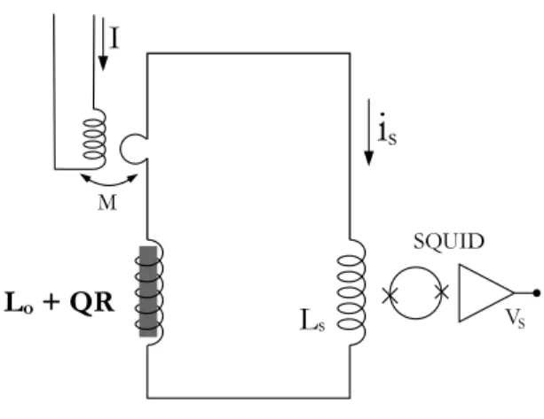
Figure 2. Circuit allowing fluctuation and response measurements (absolute thermometer).
where R(t′
, t) is the averaged one site response function of the sample. If a current i is flowing in the coil, the flux on the coil due to the polarization of the sample reads
Φ(t) =X i X µ hµi2 Z t R(t′ , t)i(t′ )dt′ . (9)
Thus, the response function of the flux due to the sample in the PU circuit is RΦ(t
′
, t) = QR(t′
, t). (10)
The same coupling factor Q =P
i P µh µ i 2
determines the values of correlation and response of the flux due to the sample.
Note that the term h is the value of the internal field in the sample, due to a unit of current flowing in the coil. Therefore, Q corresponds to the same demagnetizing field conditions in both measurements. Actually, Q is time dependent, since the internal field is hint= h0µ(t′, t) where µ(t′, t) is the time dependent sample permeability,
but the important point is that Q(t′
, t) is exactly the same in both experiments.
The above derivation is done in the context of a magnetic system, showing that the measured quantities represent those used in theoretical works. Incidentally, equivalent derivation could be done for any system with magnetic response, for instance the eddy currents in a conductor, with the same result: the coupling factors are the same in the fluctuations and the response.
The basic measurement circuit is depicted in Fig. 2. A small coil coupled to an excitation winding with mutual inductance M is inserted in the PU circuit. The total flux impulse response of the circuit to the current i(t′ ) flowing in it is RL(t′, t) = X Lδ(t − t′ ) + Q(t′ , t)R(t′ , t), (11)
whereP L is the total self inductance of the circuit. Flux conservation in the (SC) PU circuit leads to
Φexc(t) + Z t −∞ RL(t ′ , t)i(t′ )dt′ = 0, (12)
where Φexc(t) = M I(t) is obtained by injecting a current I(t) in the excitation winding. The conjugate variable
of the circuit current i is the flux Φexc injected by the excitation coil.
The properties of the system are easy to derive in the case of an ergodic sample. By time translational invariance, Eq. 12 can be transformed into the frequency regime as ˜Φexc(ω) + ˜RL(ω)˜i(ω) = 0 where ˜x represents
the Fourier transform of x, leading to the current response function to flux excitation: ˜ Ri(ω) = − 1 ˜ RL(ω) = −P L + ˜Q(ω) NR˜∗ (ω) ˜ RL(ω) ˜R∗L(ω) . (13)
Since ˜Q(ω) is a real quantity,
ℑ ˜Ri(ω) = ˜ Q(ω)N ℑ ˜R(ω) ˜ RL(ω) ˜R∗L(ω) . (14)
The ergodic sample obeys FDT,
˜
C(ω) ≡ S(ω) = 2kBT
πω ℑ ˜R(ω), (15)
where S(ω) is the magnetic fluctuations power spectrum. Thus, by using Eq. 14, one finds the circuit current noise power spectrum:
Si(ω) = ˜ Q(ω)NS(ω)˜ ˜ RL(ω) ˜R∗L(ω) = 2kBT πω ℑ ˜Ri(ω). (16) Thus, fluctuations and response of the circuit current obey also the FDT relation. Translation into the time domain follows classically:
σi(t − t ′ ) = 1 kBT Ci(t − t ′ ). (17)
The SQUID gain is G = VS/i. Thus, if a current I(t) = I0(1 − θ(t)) is injected in the excitation coil, the
relaxation of the SQUID output voltage is related to its fluctuations autocorrelation function by VS(t) = M I0 G 1 kBT hVS(0)VS(t)i . (18)
The system is an absolute thermometer since, by measuring both the response voltage to an excitation current step and the autocorrelation of the voltage free fluctuations, it allows a determination of the temperature whose precision (once a sample with large signal is chosen) depends only on the precision of the determination of the experimental parameters I0, G and M .
In the case of a non-stationary sample, things are of course more complex. Nevertheless, it is possible to analyze the case of a system with only one timescale (or correlation scale) in the large t′
limit. In that case, X(C) = X1 < 1 for C < qEA, and the time can be re-parametrized9 such that R(t′, t) ≡ R(λ(t) − λ(t′)) and
C(t′ , t) ≡ C(λ(t) − λ(t′ )) yielding χ(λ − λ′ ) = βX1 Z qEA C(λ−λ′) dC + βqEA= β(1 + X1)qEA− βX1C(λ − λ ′ ). (19)
Therefore, time translational invariance is recovered “in λ”. The behavior of the thermometer can be analyzed in the same way than in the ergodic case, showing that the measured response will vary linearly as a function of the measured correlation with slope M I0
G X1β. According to mean field predictions,
13 this could be true within
any timescale in a multi-timescale system.
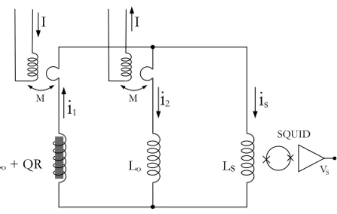
The main drawback of the elementary measuring circuit depicted above is that the response to an excitation step involves the instantaneous response of the total self inductance of the circuit (first term in the right hand side —R.H.S— of Eq. 11). In our case, both the susceptibility of the sample and the coupling factor Q are weak. The quantity to be measured,— the second term in the R.H.S of Eq. 11—, represents a few percent of the first one. Thus, a bridge configuration depicted in Fig. 3 has been adopted. Now, the main branch involving the sample is balanced by an equivalent one without sample. This second branch is excited oppositely, in such a way that when the sample is extracted from the PU, there is no response of the SQUID to an excitation step. When the sample is placed into the PU, the response of the SQUID is determined only by the response of the sample. Nevertheless, now, the loop coupling factor of the sample to the SQUID involves different self inductance terms in both measurements, and one gets
VS(t) = M I0 G L0 L0+ 2LS 1 kBT hVS(0)VS(t)i , (20)
Figure 3. Balanced configuration circuit.
where L0 and LS are the self inductances of the PU and of the SQUID input respectively, and the effect of
the sample has been neglected in the value of L0. This adds sources of error on the calibration since the self
inductance values are difficult to determine precisely.
Thus the thermometer was calibrated by using a perfect ergodic system, a cylinder of pure copper with very high conductivity (ρ300K/ρ4.2K > 1000). At 4.215K (4He boiling temperature at normal pressure) the SQUID
signal fluctuations autocorrelation was determined by standard FFT algorithms, and the relaxation after an excitation step was recorded. As can be seen in Fig. 5, the dynamics in the copper does not exceed times of order 1 s, and the signal/noise ratio is very large. The measurement is very easy. The result is depicted on Fig. 4 where relaxation data are plotted versus correlation ones. Except for the few points at the largest C (shortest times, where the effect of the filters in the current excitation circuit is apparent), the relation between both measured quantities is linear with slope A/T , where A = M I0
kBG
L0
L0+2LS is the sample independent calibration factor. This factor can thus be determined from the measurement, since the temperature is known. From the knowledge of the numerical value of A, the experimental FDT slope is known exactly at any temperature and for any sample.
0.0 10.0µ 20.0µ 30.0µ 0.0 0.5 1.0 1.5 2.0 2.5 Cu 4.2K Slope A/T VS ( V ) <VS(t) VS(0)> (V2)
3.2. The thiospinel sample CdCr
1.7
In
0.3S
4The FD relation was investigated in the insulating thiospinel spin glass CdCr1.7In0.3S4. The pure Cr compound
is a ferromagnet where the Cr3+ ions have ferromagnetic interactions between nearest neighbors, and
antifer-romagnetic ones between next nearest neighbors. Substitution of Cr by In introduces disorder and frustration since it favorises the antiferromagnetic interactions. The compound enters a spin glass phase below a transition temperature Tg = 16.7K.20 Just above Tg, the susceptibility is Curie-Weiss like, with a Curie constant
corre-sponding to ferromagnetic clusters of about 50 spins, and a small antiferromagnetic interaction between clusters (θ = −22K). This clustering complicates the analysis of the experimental results as will be shown below, but it is the reason of the large susceptibility and fluctuations amplitude, allowing good noise measurements which would be impossible in a canonical metallic spin glass in the present state of the experimental possibilities. Extensive investigations of the aging properties of the magnetic response were performed in this compound: aging of TRM relaxation21 and of the out-of-phase susceptibility22 , effect of the temperature variations.23 With it, the first
(and probably the only) systematic measurement of the aging of the magnetic noise power spectrum in a spin glass was performed by collecting an ensemble average of noise power at 10−2Hz. This allowed a qualitative
comparison with the results of out-of-phase susceptibility aging at the same frequency, showing that, in the quasi-stationary regime (ωt ≫ 1), FDT was approximately valid.22
3.3. Experimental methods and results
The enormous difficulty of the experiment lies in the extreme weakness of the amplitude of the magnetic fluctu-ations in the sample: in our case, it corresponds to the response of the sample to a field about 10−7G. As it is
quite impossible to suppress the ambient field at such a level, the solution is twofold. First to reduce it at a level of order 1mG and stabilize it as best as possible: this is obtained by isolation and shielding procedures which will not be developed further here. Second, to use a gradiometric PU coil: a third order gradiometer made of +3, -6, +6, -3 turns in an Helmoltz geometrical configuration (see Fig. 1), as used in our experiment, suppresses the effect of the field up to second order and all even orders. The result can be seen on Fig. 5 where the r. m. s. noise spectra of the system in several cases are displayed. The free SQUID level is the absolute background of sensitivity. Once added the empty measuring coils equipment, the low frequency noise is slightly higher, with a slope sightly sharper than 1/f . Also represented is the spectrum recorded with the sample at 0.8Tg. One can see
that the magnetic fluctuations of the sample in this range of temperatures give a signal more than 20 dB above the proper noise of the system, at least for time analysis up to several thousands of seconds. It can be seen also that this is not the case for low temperatures (see 4.2 K in the figure). The problem is that the correlation is sensitive to all time scales. As the slope of the sample power spectrum is less than 1/f , the signal/noise ratio is going to be unfavorable at very long times above ten thousand seconds.
Another non negligible difficulty is that in a non-stationary system, the time autocorrelation of magnetic fluctuations must be determined as an ensemble average over a large number of equivalent records of the fluctu-ations signal, each one initiated by a quench from above Tg(“birth” of the system). This makes the experiments
very long, and complicates them strongly since a perfect reproducibility of the temperature history in the cooling procedure must be obtained.
In the present work, the time autocorrelation hVS(t′)VS(t)i and the relaxation VS(t′, t) were measured after
quench from an annealing temperature T ≃ 1.2Tg to working temperatures T = 0.6Tg, 0.8Tg and 0.9Tg. In the
relaxation experiments, the excitation current was such that the excitation field in the sample was less than 1mG. The cooling procedure was the following: first slow cooling from the annealing temperature to 3K above working temperature, and then fast quench to the working temperature. This procedure was chosen in order to reduce the perturbation of the cryogenic bath —which would lead to SQUID instabilities—, while keeping a definition of the time zero (“birth” time) within less than 10s error.
The autocorrelation was determined from an ensemble average of up to 350 records of the fluctuation signal after quench, with length up to 12000s. The SQUID output voltage antocorrelation C(t′
, t) was computed as a function of t−t′
for values of t′
from 100s to 10000s. To improve the averaging convergence, the ensemble averages were computed using short time averages of the signal at t′
and t in each record. The best compromise allowing a good average convergence, still being compatible with non-stationarity was δt′
≤ t′
/20 and δt ≤ (t − t′
10-5 10-4 10-3 10-2 10-1 100 101 102 103 1E-5 1E-4 1E-3 0.01 0.1 Cu 4.2K Sample 4.2K Sample 0.8Tg System empty SQUID
N
o
is
e am
p
lit
ude
,
Φ
0/H
z
1 /2Frequency (Hz)
Figure 5. Noise power spectra of the measuring system in different configurations.
there is an arbitrary offset on the SQUID signal (due to the SQUID itself, as well as to the effect of the residual field on the sample), the connected correlation was computed:
CV(t′, t) = h(VS(t′) − hVS(t)i) (VS(t) − hVS(t)i)i (21)
Nevertheless, the above procedure cannot suppress a random offset in the results, due to fluctuating modes of period much longer than 2000s. These modes involve not only the fluctuating signal of the sample but also uncontrolled long timescale drifts of the measurement setup. As it is impossible to disentangle both contributions, the correlation data have been normalized by taking as the origin the value ofV2
S(t ′
)®. Due to the elementary measurement time constant, this term corresponds to an average over t − t′
about 10−2s i.e. a range of (t − t′
)/t′
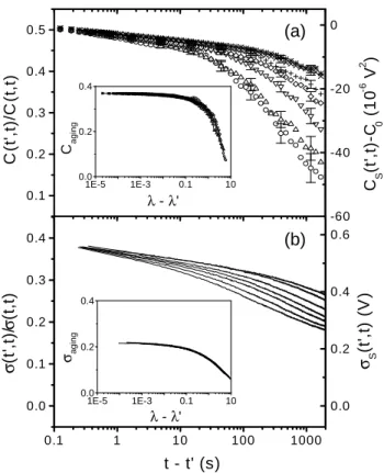
corresponding to the stationary regime where all C curves must merge. This amounts to shifting all the data by a common unknown offset C0. The result at T = 0.8Tgis shown on Fig. 6.a (right sided scale), as a function
of t − t′
and for all chosen values of t′
. Residual oscillations —and large error bars— in the curves at lowest t′
reveal the limit of efficiency of the averaging procedure.
In comparison with the above, the measurement of relaxation is very easy. The relaxation curves at 0.8Tg
are plotted on Fig. 6.b. In both results, the curves merge at small t − t′
, meaning that they do not depend on t′
(stationary regime). At t − t′
≫ t′
, they strongly depend on t′
, the slower decay corresponding to the longer t′
: the curves follow roughly a (t − t′
)/t′
scaling in the aging regime. Yet at this stage, a point can be stressed: the experimental waiting times t′
are not long enough for timescales separation since it is apparent on the curves that the non-stationary regime begins while the stationary relaxation has not ended.
4. DISCUSSION: THE FLUCTUATION DISSIPATION GRAPH
Experimental results can be represented on a σ(C) plot (plot of σ(C) for each t′
, using t as parameter) following the ideas of Cugliandolo and Kurchan. The inset in Fig. 7 displays the results at 0.8K plotted in experimental units for C, and in reduced units for σ (since the experimental value of χF C is known). A clear linear range
appears at large correlation (small t−t′
). In the figure, the FDT slope, computed from the value of the calibration factor A is represented by the full straight line. The data display the FDT slope with less than 3% error in the sector of large correlation corresponding to a reduced correlation C/C(t, t) ≥ 0.47. Now, the correlation offset must be suppressed. As correlation zero is unreachable in experimental times, suppression of the offset could be obtained from the knowledge of C(t, t) (square of the moment of the elementary fluctuator). Unfortunately, due to
1E-5 1E-3 0.1 10 0.0 0.2 0.4 Cagi ng λ - λ' 0.1 0.2 0.3 0.4 0.5 C (t ',t) /C (t ,t) -60 -40 -20 0 C S (t ', t)-C 0 ( 10 -6 V 2 ) 1E-5 1E-3 0.1 10 0.0 0.2 0.4 σagi n g λ - λ' 0.1 1 10 100 1000 0.0 0.1 0.2 0.3 0.4 t - t' (s) σ (t ',t) / σ (t ,t ) 0.0 0.2 0.4 0.6 σ S (t ',t ) (V )
(a)
(b)
Figure 6. a) Correlation and b) Relaxation measured at 0.8Tg. The curves correspond to t
′ from 100s to 10000s from
top to bottom. In the insets, scaling plots of the non-stationary contributions.
clustering, C(t, t) depends on temperature and cannot be determined from the high temperature susceptibility. To obtain an evaluation of C(t, t), an ansatz inspired by the properties of the canonical compounds like 1% Cu:Mn24 was used. In these compounds with negligible clustering, the field cooled (FC) susceptibility is Curie
like above Tgand temperature independent below Tg, yielding C(t, t) = TgχF C(T ). The ansatz consists in using
a generalization of this relation with the condition that a monotonous dependence of C(t, t; T ) must result. This is obtained by using for Tg a slightly different value Tg∗= 17.2K. Then, writing C(t, t; T ) = 17.2χF C(T ),
C(t, t; T ) can be obtained and suppression of the offset can be performed using the σ(C) plot by the following procedure. One plots the normalized susceptibility function ˜χ(t′
, t) = 1− ˜σ(t′
, t) where ˜σ(t′
, t) = VS(t′, t)/VS(t, t)
(note that VS(t, t) is the FC (initial) value of the relaxation SQUID signal), versus normalized autocorrelation
˜ C(t′
, t) − ˜C0= (CS(t′, t) − C0)/CS(t, t; T ) where CS(t′, t) = hVS(t′)VS(t)i. In this graph, the FDT line has slope
−T∗
/T and crosses the ˜C axis at ˜C = 1. The result is shown on Fig. 7 for all investigated temperatures. It is of course based on a rough ansatz on C(t, t; T ) which needs further justifications, but the resulting uncertainty concerns only the position of the zero on the ˜C axis, and not the shape and slope of the curves. With decreasing
˜
C (increasing t − t′
≥ t′
), the data points depart from the FDT line. Despite the scatter of the data, a t′
dependence in the non-FDT regime is clear: the data at small t′
depart the FDT line at larger values of ˜C. This is the consequence of the non-separation of the timescales in the range of the experimentally accessible values of t′
. Even if the long t′
limit for ˜χ( ˜C) does exist, it is not reached in the results of Fig. 7.b and a t′
dependence of the ˜χ( ˜C) curves is expected.
Further insight would result from the separation of stationary and non-stationary contributions in the data. In the “weak ergodicity breaking” scenario, the relaxation and correlation can be written as the sum of two parts, a stationary one and a non-stationary one.9 For instance:
˜ C(t′ , t) = (1 − qEA)Fstat(t − t ′ ) + qEAFaging(t ′ , t). (22)
0.0
0.2
0.4
0.6
0.8
1.0
1.0
0.8
0.6
0.4
0.2
0.0
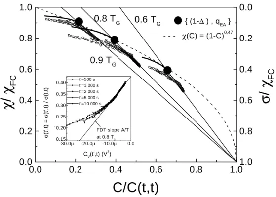
- - - χ(C) = (1-C)0.47 { (1-∆ ) , qEA }0.9 T
G0.8 T
G0.6 T
Gσ
/
χ
F
C
C/C(t,t)
0.0
0.2
0.4
0.6
0.8
1.0
χ
/
χ
F
C
-30.0µ -20.0µ -10.0µ 0.0 0.15 0.20 0.25 0.30 0.35 0.40 FDT slope A/T at 0.8 Tg ~ σ (t ',t ) = σ (t ',t ) / σ (t,t) CV(t',t) (V 2 ) t'=500 s t'=1 000 s t'=2 000 s t'=5 000 s t'=10 000 sFigure 7. χ˜vs. ˜C plots at 0.6, 0.8 and 0.9Tg. In the inset, σ vs. C plot of the data at 0.8Tg, with C in experimental
units.
of large t′
where both timescales are separated but is questionable otherwise. Indeed, it would lead, in case of very long tail in the stationary correlation, to a stationary regime after the end of the non-stationary one. More probably, in the mixed timescales regime, both contributions are more intricate than a simple addition. A first step to take it into account is to adopt a multiplicative formulation. For instance:
˜ C(t′ , t) = ((1 − qEA)Fstat(t − t ′ ) + qEA)Faging(t ′ , t) (23)
Note that for very large t′
such that Fstat(t′) → 0, one recovers Eq. 22. During the last decade, a form of scaling
was used successfully to analyze aging relaxation.9 Inspired by the old work of Struik8on glassy polymers, this
scaling corresponds in fact to one timescale time re-parametrization.9 Applied to Eq. 23 for ˜σ, it leads to :
˜ σ(t′
, t) = ((1 − ∆)(1 + (t − t′
)/t0)−α+ ∆)ϕ(λ(t) − λ(t′)) (24)
where t0 is an elementary time of order 10−10s, ϕ is a scaling function of an effective time λ(t) = t1−µ/(1 − µ)
depending on the subaging coefficient µ < 1, and α can be determined with good precision from the stationary power spectrum of fluctuations S(ω) ∝ ωα−1. The inset on Fig. 6.b displays the scaling of the aging part of the
relaxation curves at 0.8Tg. As shown in the inset of Fig. 6.a, the scaling works rather well on the autocorrelation
data with the same exponents, but now, qEAreplaces ∆. If granted, the scaling would allow an artificial separation
of the timescales, by separating stationary (short timescale) and non-stationary (all timescales) contributions. The smoothed curves ˜χaging( ˜Caging) are plotted on Fig. 7 at each temperature, as well as the points {(∆), qEA}
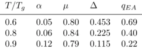
also given in Table 1.
Our results seem to rule out any interpretations in terms of simple domain growth models, like the “disguised ferromagnet” of Fisher and Huse.26 It seems clear that the dynamics does not seem to approach a limit in which
the relaxation would stop at the end of the FDT regime, leading to an infinite effective temperature in the aging regime. Nevertheless, it must be noted that, due to the limited values of our waiting times t′
, our results are not contradictory with the predictions of a recent very sophisticated modified version of the droplet model.27
Table 1. Values of the fit parameters at the three investigated temperatures.
T /Tg α µ ∆ qEA
0.6 0.05 0.80 0.453 0.69 0.8 0.06 0.84 0.225 0.40 0.9 0.12 0.79 0.115 0.22
On the contrary, as shown above, a time scaling reminiscent to one-step replica symmetry breaking (RSB) — or one timescale— models9 seems to describe rather correctly the relaxation and correlation data, at least
in all our experimental times. Our system has a strong heisenberg character,28 and it has been shown that
in such case, the spin glass transition should correspond to chiral ordering with one-step RSB.28, 29 Numerical
simulations on an heisenberg system with weak anisotropy have been performed recently,30 whose results are characteristic of one RSB, with Tef f higher than but independent of the bath temperature: in other words, a
“universal” —constant Tef f— ˜χ( ˜C) curve is obtained. In a one-RSB system, it can be shown that ∆ and qEA
are related simply by qEA = 1/(1 + γT /Tef f) where γ = (1 − ∆)/∆. If we use the values given in Table 1, we
obtain for Tef f the values 1.25Tgat T = 0.6Tg, 1.6Tg at T = 0.8Tg and 1.8Tg at T = 0.9Tg, i. e. a non-universal
behavior. On the other hand, our non-stationary ˜χ( ˜C) curves does not fit the above values. They start with higher slope and bend downward. An experimental bias cannot be excluded a priori, but it can be remarked that this is not coherent with the data: the bend down effect is the largest at the highest temperature, i.e. when the amplitude of fluctuations is the largest (best signal/noise ratio) and the perturbation of the measuring system by the quench is the smallest. If we take an average slope of the re-scaled aging parts in the ˜χ( ˜C) diagram, we obtain 2.4, 3.2 and 4Tg. Thus, our result, though derived on the basis of a one RSB scaling, does not seem to
be fully coherent with one-RSB hypothesis.
The possibility of multiple (or continuous) RSB cannot be excluded. On the basis of the PaT hypothesis, in the mean field SK model, the χ(C) curve is temperature independent. It can be described by χ = (1 − C)0.5, at
large correlations,25 and at small correlations it is assumed to follow a behavior like 1 − χ ∝ C2, insuring that
X(C) ≡ x(q) has zero slope at the origin, or in other words that there is no peak of the distribution P (q) at q = 0. It has been shown recently by numerical simulations that in short range models and for large correlations, a generalized relation like χ = A(1 − C)Bwith B < 1 is more adequate.19 Rather remarkably, in Fig. 7, the points
{(1 − ∆), qEA}, as well as the beginning of the ˜χ( ˜C) curves (short times) are well described by ˜χ( ˜C) = (1 − ˜C)0.47
(dashed curve in the figure), a relation very close to the mean field one. This apparent conformity with a mean field prediction is rather astonishing for a real material, but it must be noted that here, it applies in the range of small correlations, leading to non-zero slope at ˜C = 0. Moreover it is contradictory with the fact that the exponent of the stationary relaxation α ≤ 0.1 is very small, while the mean field prediction is α = 0.5. At large times, (small correlation) the ˜χ( ˜C) data curves separate from the dashed curve, tending to a smaller slope, and they point to values smaller than 1 on the ˜χ axis. In the continuous RSB case, one can expect that the ˜χ( ˜C) curves tend to zero derivative at the origin, which is the tendency in the results. It remains that the scaled plots are not aligned correctly as to describe a continuous ˜χ( ˜C) curve. One could argue that in a context of continuous RSB, the one-RSB scaling cannot allow a correct separation of stationary and non-stationary contributions and does not reach the real limit for full time-scale separation.
5. CONCLUSION
The ensemble of results reported here represents the first experimental determination of the time autocorrelation of the magnetic fluctuations in the strong aging regime of a spin glass. The task of the experiment was to compare quantitatively the time autocorrelation of fluctuations and the relaxation. This was made possible by reconsidering in detail the experimental principles: the physical problem being fundamentally connected with the thermodynamic definition of the temperature, the experimental setup might be understood as an absolute thermometer.
Our results differ substantially from what could be predicted on the basis of domain growth models. They are summarized on the ˜χ( ˜C) graph displayed in Fig. 7. Comparison is made with predictions based on
one-RSB and continuous one-RSB. Due to the strong heisenberg character of CdCr1.7In0.3S4, chiral ordering with
one-RSB could seem the more realistic for this compound. In fact, the precision of our data does not allow us to discriminate between both models. Due to the non-canonical nature of the insulating compound investigated, the interpretation of the results needed the use of an hypothesis which is far for being justified at the theoretical level: the ansatz used to determine C(t, t; T ) is rather rough; an experimental determination, by neutron diffraction techniques for instance, is needed for a more rigorous interpretation of the data.
ACKNOWLEDGMENTS
We thank J. Hammann, E. Vincent, L. F. Cugliandolo, J. Kurchan, M. V. Feigel’man, L. B. Ioffe and particularly G. Parisi for enlightening discussions.
REFERENCES
1. H. B. Callen and T. A. Welton, “Irreversibility and generalized noise,” . Phys. Rev. 83, pp. 34-40, (1951). 2. R. Kubo, “Statistical-mechanical theory of irreversible processes,” J. Phys. Soc. Jpn. 12 pp. 570-586, (1957). 3. M. Ocio, H. Bouchiat and P. Monod, “Observation of 1/f magnetic fluctuations in a spin glass,” J. Phys.
Lettres 46, pp. L647-L652, (1985).
4. M. Ocio, H. Bouchiat and P. Monod, “Observation of 1/f magnetic fluctuations in spin glasses,” J. Mag. Mag. Mat. 54-57, pp. 11-16, (1986).
5. P. R´efr´egier, M. Ocio and H. Bouchiat, “Equilibrium magnetic fluctuations in spin glasses: temperature dependence and deviations from 1/f behavior,” Europhys. Lett. 3, pp. 503-510, (1987).
6. L. Lundgren, P. Svedlindh, P. Nordblad and O. Beckman, “Dynamics of the relaxation-time spectrum in a CuMn spin-glass,” Phys. Rev. Lett. 51, pp. 911-914, (1983).
7. M. Ocio, M. Alba and J. Hammann, “Time scaling of the aging processin spin-glasses: a study in CeNiFeF6,”
J. Phys. Lettres 46, pp. L1101-L1107, (1985).
8. L. C. E. Struik, Physical Ageing in Amorphous Polymers and Materials, Elsevier Scientific Publ., Houston Tex. (1978).
9. For a review, see E. Vincent, J. Hammann, M. Ocio, J. P. Bouchaud and L. F. Cugliandolo, “Slow dynamics and aging in spin glasses” in Complex Behavior of Glassy Systems, Springer Verlag Lecture notes in Physics Vol. 492, M. Rubi Edt., pp. 184-219, (1997).
10. For a review, see M. M´ezard, G. Parisi and M. A. Virasoro, Spin Glass Theory and Beyond, World Scientific Lecture Notes in Physics Vol. 9 (1987).
11. V. Dupuis, E. Vincent, J. P. Bouchaud, J. Hammann, A. Ito and H. Aruga Katori, “Aging, rejuvenation, and memory effect in Ising and Heisenberg spin glasses,” Phys. Rev. B 64, pp. 174204 1-7, (2001).
12. L. F. Cugliandolo and J. Kurchan, “Analytical solution of the off-equilibrium dynamics in a long-range spin-glass model,” Phys. Rev. Lett. 71, pp. 173-176, (1993).
13. L. F. Cugliandolo and J. Kurchan, “On the out-of-equilibrium relaxation of the Sherrington-Kirkpatrick model,” J. Phys A 27, pp. 5749-5772, (1994).
14. J. P. Bouchaud, “Weak ergodicity breaking and aging in disordered systems,” J. Phys. (France) I 2, pp. 1705-1713, (1992).
15. L. F. Cugliandolo, J. Kurchan and L. Peliti, “Energy flow, partial equilibration and effective temperature in systems with slow dynamics,” Phys. Rev. A 55, pp. 3898-3914, (1997).
16. G. Parisi, “Magnetic properties of spin glasses in a new mean field theory,” J. Phys. A 13, pp. 1887-1895, (1980).
17. G. Parisi and G. Toulouse, “A simple hypothesis for the spin glass phase of the infinite ranged S-K model,” J. Phys. Lettres 41, pp. L361-L364, (1980).
18. S. Franz, M. M´ezard, G. Parisi and L. Peliti, “Measuring equilibrium properties in aging systems,” Phys. Rev. Lett. 81, pp.1758-1761, (1998).
19. E. Marinari, G. Parisi, F. Ricci-Tersenghi and J. J. Ruiz-Lorenzo, “Off-equilibrium dynamics at very low temperatures in three-dimensional spin glasses,” J. Phys. A 33, pp. 2373-2382, (2000).
20. E. Vincent and J. Hammann, “Critical behavior of the Cd2×0.85In2×0.15Cr2 S4 insulating spin glass,” J.
Phys. C 20. pp. 2659-2672, (1987).
21. M. Alba, J. Hammann, M. Ocio, P. R´efr´egier and H. Bouchiat, “Spin glass dynamics from magnetic noise, relaxation and susceptibility measurements,” J. Appl. Phys. 61, pp.3683-3687, (1987).
22. P. R´efr´egier, M. Ocio, J. Hammann and E. Vincent, “Non-stationary dynamics from susceptibility and noise measurements,” J. Appl. Phys. 63, pp. 4343-4345, (1988).
23. P. R´efr´egier, E. Vincent, J. Hammann and M. Ocio, “Ageing phenomena in a spin-glass: effect of temperature changes below Tg,” J. Physique 48, pp. 1533-1539, (1987).
24. S. Nagata, P. H. Keesom and H. R. Harrison, “Low-dc-field susceptibility of CuMn spin-glass,” Phys. Rev. B 19, pp. 1633-1638, (1979).
25. E. Marinari, G. Parisi, F. Ricci-Tersenghi and J. Ruiz-Lorenzo, “Violation of the fluctuation-dissipation theorem in finite-dimensional spin glasses,” J. Phys. A 31, pp. 2611-2620, (1998).
26. D. S. Fisher and D. A. Huse, “Nonequilibrium dynamics of spin glasses ” Phys. rev. B 38, pp. 373-385, (1988).
27. H. Yoshino, K. Hukushima and H. Takayama, “Extended droplet theory for aging on short-range spin glasses and a numerical examination,” Phys. Rev. 66, pp. 064431 1-26, (2002).
28. D. Petit, L. Fruchter and I. A. Campbel, “Ordering in heisenberg spin glasses,” Phys. Rev. Lett. 88, pp. 207206/1-4, (2002).
29. K. Hukushima and H. Kawamura, “Chiral-glass transition and replica symmetry breaking of a three dimen-sional heisenberg spin glass,” Phys. Rev. E 61, pp. R1008-11, (2000).