RECURSION-BASED MULTIPLE CHANGEPOINT DETECTION IN
MUL TIV ARIA TE LINEAR REGRESSION AND APPLICATION TO RIVER STREAMFLOWS
Recursion-based Multiple Changepoint Detection in Multivariate Linear
Regression and Application to River Streamflows
O. Seidou*, T.B.M.J. Ouarda,
INRS-ETE, Hydro-Québec NSERC Chair in Statistical Hydrology/Canada Research Chair on the Estimation ofHydrological Variables, 490 rue de la Couronne, Quebec (QC), Canada GIK 9A9
Rapport de recherche R-843
Submitted to Water ReS"ources Research March 2006
*Corresponding author: Tel: (418) 654-2542 Fax: (418) 654-2600
Abstract
A large number of models in hydrology and c1imate SCIences rely on multivariate linear regression to explain the link between key variables. The relationship in the physical world may experiment sudden changes due to c1imatic, environmental or anthropogenic perturbations. To deal with this issue, a Bayesian method of multiple changepoint detection in multivariate linear regression is proposed in this paper. It is an adaptation of the recursion-based multiple changepoint method of Fearnhead [2005] to the c1assical multivariate linear mode!. A new c1ass of priors for the parameters of the multivariate linear model is introduced and useful formulas are derived that permit straightforward computation of the posterior distribution of the changepoints. The proposed method is numerically efficient and does not involve time consuming Monte-Carlo Markov Chain simulation as opposed to other Bayesian changepoint methods. It allows fast and straightforward simulation of the probability of each possible number of changepoints as weIl as the posterior probability distribution of each changepoint conditional on the number of changes. The approach is validated on simulated data sets and then compared to the methodology of Asselin and Ouarda [2005] on two practical problems: a) the changepoint detection in the multivariate linear relationship between mean basin scale precipitation at different periods of the year and the summer-autumn flood peaks of the Broadback River located in Northem Quebec, Canada; and b) the detection of trend variations in the streamflows of the Ogoki River located in the province of Ontario, Canada.
Keywords: Bayesian analysis, changepoint, hydrology, streamflows, multivariate linear regresslOn.
1. Introduction
An increasing number of papers point out shifts or trends in hydrologie time series [e.g. Burn and Elnur, 2002; Woo and Thorne, 2003; Salinger, 2005]. A change ofmentality is taking place in the whole scientific community and it is probable that hydrologie time series models which do not hold account of a possible change in the statistical distribution of the data will no longer be regarded as credible. Detection of eventual changes in collected data sets is thus obviously an important step before performing any descriptive or predictive analysis.
Changepoint analysis is addressed both in Classical and Bayesian statistics. Methods in c1assical statistics usually consist ofperforming several kinds of tests to confirm or reject the hypothesis of change. Most ofthem address slope or intercept change in linear regression models [Solow, 1987; Easterling and Peterson, 1995; Vincent, 1998; Lund and Reeves, 2002; Wang, 2003].
In Bayesian statistics, one is interested in obtaining a statistical distribution for the dates of change and eventually a distribution for the other model parameters. Bayesian changepoint analysis models are the subject of a large number of papers [e.g. Booth and smith, 1982; Bruneau et Rassam, 1983; Gelland et al. 1990; Barry and Hartigan, 1992, 1993; Stephens, 1994; Perreault et al., 2000a,b,c; Rasmussen, 2001]. More recently, Asselin and Ouarda [2005] developed an approach to changepoint detection in multivariate linear relationships and Fearnhead [2005] proposed a recursion-based inference procedure based on the theory of product-partition models [Barry and Hartigan, 1992,1993] for multiple changepoint problems. In the latter paper, a set of recursive relations are used to infer the posterior probabilities of different numbers of changepoints. A particularity of this approach is that it focuses only on the number and positions of changes.
The aim of this paper is to adapt the methodology of Fearnhead [2005] to multiple changepoint detection in multivariate linear relations. In particular, a special class of priors for the parameters of the multivariate linear model is introduced and useful formulas are derived that permit straightforward computation of the posterior distribution of the changepoints. The proposed methodology is validated on simulated data sets to prove its ability to infer the number and location of changepoints. It is then applied to two case studies. In the first case study, the summer-autumn flood peaks of the Broadback River located in the province of Quebec, Canada, are investigated for the eventual changes due to forest fires. The second case study deals with the detection of eventual trend variations in the streamflow data of the Ogoki River located in the province of Ontario, Canada.
As the first case study has aIready been investigated with a changepoint detection approach using Gibbs sampling [Asselin and Ouarda, 2005; Seidou and Ouarda, 2005], the results obtained with the two methodologies will be compared and discussed in this paper. The approach of Asselin and Ouarda [2005] will also be applied to the second case study in order to highlight the importance ofhaving a methodology designed to handle several changepoints.
The outline of the paper is as follow: Section 2 is a quick survey of changepoint detection methodologies with an emphasis on Bayesian methodologies with application to hydrological problems. Section 3 is devoted to the methodology of Asselin and Ouarda [2005] which will be compared to the proposed approach. Recursion based changepoint inference models are introduced in Section 4, and the model of Fearnhead [2005] is adapted to multivariate linear regression. The simulation of changepoints given the conditional posterior probabilities of the dates of change is presented in Section 5. The simulation-based validation methodology is presented in section 6. Section 7 presents the results of the simulation studies and the applications
on real data are carried out in section 8. A conclusion and sorne recommendations are finally presented in Section 9.
2. Changepoint models
Changepoint detection has received a great de al of attention in statistical literature because modification of model structure and/or parameters is commonly encountered in applied statistics (e.g in finance, pharmacology, econometrics, hydrology, etc.). The change detection can be off-line (or retrospective) or onoff-line (or sequential) when it is important that the change be detected as soon as it occurs. Examples of online changepoint detection methods can be found in [Lai, 1995; Beibel, 1997; Daumer and Falk, 1998; Gut and Steinebach, 2002; Daumer and Falk, 1997; Moreno et al, 2005].
Most applications in hydrology are used for retrospective changepoint detection, except a few ones [e.g. Moreno et al, 2005]. Retrospective changepoint detection methods often use classical statistical methods to detect changes in slopes or intercepts of linear regression models [Solow, 1987; Easterling and Peterson, 1995; Vincent, 1998; Rasmussen, 2001; Lund and Reeves, 2002; Wang, 2003]. Other curve fitting methods are used in sorne rare cases [e.g. Sagarin and Micheli, 2001; Bowman et al., 2004].
A growing number of methodologies use Bayesian statistics. Gelfand et al [1990] discussed Bayesian analysis of a variety of normal data models, including regression and ANDV A-type structures, where they allowed for unequal variances. Barry and Hartigan [1992, 1993] used product-partition models to develop a Bayesian analysis for a multiple changepoint problem that can be exactly solved using a finite number of operations. The multiple changepoint component was introduced by a normal random variable that can be added anytime to the mean of the series, but only with a certain probability. Stephens [1994] implemented Bayesian analysis of a multiple
changepoint problem where the number of changepoints is assumed known, but the times of occurrence of the changepoints remain unknown. Other authors emphasized on the single changepoint problem. We cite for example Carlin et al. [1992] who applied a three-stage hierarchical Bayesian analysis to a simple linear changepoint model for normal data: ~ON[al+blxl,JI2], t=l, ... ,r, ~DN[a2+b2xt'J~], t=r+l, ... ,n. Perreault et al. [2000a; 2000b] gave Bayesian analyses of several changepoint models of univariate normal data. AIl of these authors implemented their analyses using Gibbs sampling. Rasmussen [2001] considered a single changepoint in a simple linear regression model with noninformative priors and derived the exact analytical posterior distribution of the regression parameters. His model assumes that the changepoint occurred with certainty, and does not allow a clear diagnosis of the existence of the change. Perreault et al. [2000c] developed an exact analytical Bayesian analysis of a changepoint in the mean ofa series ofmultivariate normal random variables.
More recently, Asselin and Ouarda [2005] developed a practical and general approach to the single changepoint inference problem relying on Bayesian multivariate regression analysis. Their model can handle multivariate data and/or missing values and can be used with both informative and noninformative priors on the regression parameters. It was shown to be more performing than other approaches recently published in the hydrological literature [Seidou and Ouarda, 2005]. However, the approach presented in Asselin and Ouarda [2005] considers only one possible changepoint and involves relatively long MCMC simulations. The method presented in this paper is expected to handle theses two issues.
3. The changepoint model of Asselin and Ouarda [2005]
is related to the (r x dO) matrix X t by y
=
X 9(Tc )+
l ' t t t "t where l5:t5:z-c ' Z-c < t 5: n,under the constraints
[la]
[lb]
[le] In these equations as well as in the remainder of the paper, bold letters indicate vectors and matrices while the superscript T indicates the transpose. In equation [lb], Z-c is the last point of
the segment before the changepoint, and Z-c = n means that there is no change in the data series.
The dimensions of the vectors 9~Tc),
P;,
p~Po'
PI'
P
2 are respectively (d" xl), (d" xl) ,(d"xl), (d;xl), (d;xl) and (d;xl).Equation[lc]impliesthat d"=d;+d;.Itisalsoassumed that error terms
{Ut}
are independent and identically distributed following N[O,Ly ]'The model assumes a changepoint in the (d" xl) vector 9~Tc) from the (d; xl) subvector
PI
tothe (d;xl) subvector
P
2' The (d;xl) subvector
Po
is assumed to remain part of 9~Tc)throughout the observation series.
In Asselin et Ouarda [2005], sorne algebraic transformations allowed to apply sorne known results on Bayesian piecewise linear regression to Model [1] and to infer its parameters. The MCMC algorithm was also designed to account for missing data in the observations record and/or in the explanatory variables. Finally, they considered a general prior specification for regression parameters as well as for the variance structure, and used Gibbs sampling to obtain empirical
posterior distributions for each parameter. For extensive details on prior specification and
MeMe
inference for model [1] we refer the reader to the original paper.4. Recursion based changepoint inference
Although recursions have been used to make inference on the number of changepoints [Yao,
1984; Barry and Hartignan, 1992, 1993], this kind of approach has been less widely used than
MeMe
based inference. Yao [1984] was the first to show that Bayesian inference for a single shift in a normally distributed sample can be performed in a finite number of recursive operations. As the number of operations grows quickly when the length of the data series increases, he also proposed an approximate inference for which the number of operations is reduced to the order of sample size. Barry and Hartignan [1992, 1993] showed that the changepoint problem can be elegantly handled using product-partition models and generalized the results of Yao [1984] to multiple changepoints and more general prior assumptions. Product partition models assume that observations in a random partition of the data are independent, and allow the data to weight the partitions that hold. The methodologies presented in these papers under this approach allow for an efficient computation of the posterior probability of different number of changepoints using recursive relations. Fearnhead [2005] used this kind of recursive relations to develop a general inference procedure for the number and positions of the changepoints.4.1 General Inference procedure for the number and positions of the changepoints Fearnhead [2005] considered a class of multiple changepoint models for which the number of changes is unknown. Let {YpY2, ... ,Yn} be the sample, n the sample size, m the number of changepoints, rD = 0, rp ... , rm+l
=
n the changepoints and Yi:j the observations from time i to timej. We also denote g(.) the probability distribution of the time interval between consecutive changepoints and go (.) the probability distribution of the first changepoint. The
/h
segment is then Y('rj_1 +)):<j with parameter <l> j .
Assuming that the observations are independents conditional on the changepoints and parameter values, Fearnhead [2005] derived the posterior probability of the changepoints:
{
prCl") 1 Y):n)
=
pel, T))Q(T) + 1)go(T))/ Q(1)pr(Tj 1 Tj_p Y):n)
=
P(Tj_) + 1, T1)Q(Tj + 1)g(Tj - Tj_l ) / Q(Tj_) + 1)[2]
where P(t, s), s ;::: t is the probability that t and s be in the same segment: P(t,s)
=
Pr(Yt:s;t,s in the same segment)s
=
fITf(YÎ 1 <l»1l"(<l»d<l>[3]
Î=t
and Q(t) is the likelihood of the segment Yt:n given a changepoint at t -1. Q(t) t
=
1, .. , n andP(t,s), s;::: tare linked by these recursive equations: n-I Q(1)
=
LP(1,s)Q(s + 1)go(s) + P(1,n)(1-Go(n -1)) s=1 n-) Q(t)=
LP(t,s)Q(s + 1)go(s + 1-t) + pet, n)(1- G(n -t)) s=1 t twhere G(t) = Lg(i) and Go(t) = Lgo(i).
Î=I Î=)
4.2. Adaptation of the changepoint inference procedure to multivariate linear regression
[4]
Consider the np+1 series of data Yj,j=1, ... n and xij,i=1, ... ,d*;j=1, ... n wherexijis thelh value of the
lh
series of explanatory variables. The multivariate linear relationship can be represented byd' Yj
=
IBkxij +&i k=1 or y= X9+& i=
1, ... ,nThe parameter vector <1> is thus given by <1>
=
[BI B2 ••• Bd' a] and we have:1 f(Yi 1 <1»
=
J2;
exp -0.5a
27r d' Yi- IBjXij j=1 aFollowing Rasmussen [2001], we have:
From [3] and [8] we have:
2
s
P(t,s)
=
Pr(Yt:s;t,s in the same segment)=
fTIf(Yi 1 <1»7r(<1»d<1> i=tAssume that the prior depends only on a and has this particular form:
-a ( c)
a exp - - 2
7r(<1»=7r(a)=p(ala,C)= a-3 a-I 2a ,a>l,c>O
iT
c-T r(a-1) 2 [5] [6] [7] [8] [9] [10] a-3 a-I 1In equation [10], the denominator 2-2 c-Tr(a- ) is only a normalizing constant that ensures
2 +00
that
f
7r(a)da=
1. Note that when a is very large, p(a) tends towards a multiple ofa-a• oJeffrey's non infonnative prior for linear regression is p(O, 0-) oc. 0- 2 [Minka, 2001], and it is sometimes assumed in Bayesian linear regression that p(o-) oc. 0--1 [e.g. Rasmussen, 2001). Unfortunately, these kinds ofpriors are improper contrarily to the one proposed in equation [10). Basic properties of p( 0-1 a, c) are derived in Appendix 1.
Finally, the expression of P(s,t) is obtained after substituting equation [10] in equation [9] and integrating out 0- and 9 in equation [9]:
_(t-s+a)
r(t -
s
+
a)
) d'(ff(E~IEs:1
+c))
2 2 P(t,s) = (2ff 2 a-I 1( )--1
T1
1/2 a-Cff 2 XS:1X S:1 r(-2-) [11]Exhaustive details on how the expression of P(s,t) is obtained are given in Appendix 2.
5. Simulation of changepoints given the conditional posterior probabilities of the changepoints
The relations presented III Section 4 glve only the posterior probability mass of the first changepoint, and the conditional probability mass of subsequent changepoints. To make inference on the positions of changepoints, we simulate a set E
=
{Sk,k=
1: M} of M possible scatter schemes of the changepoints on the segment using the posterior probability mass of the first changepoint, and the conditional probability mass of subsequent changepoints. Indeed, M should be large enough to obtain a reliable distribution for the positions of the changepoints. The k1he1ement of E is a set of mk changepoints Sk
=
gk,12
k , ... ,1~k}.
An efficient simulation algorithm for E is given by Fearnhead [2005]:2. For t
=
0, ... , n - 2, repeat the following steps:a) Compute the number ni of samples for which the last changepoint was at time
t;
b) If ni > 0, compute Pr(z-
l
' j - l=
t'YI:n );c) Sample ni times from Pre,
l
' j - l=
t'YI:n ) and use the values to update the ni samples of changepoints which have a changepoint at timet;
This algorithm is very efficient since Pre,
l
' j - l=
t,yl :n ) has to be computed only one time regardless of the number of samples required from it. Inference on the number and positions of the changepoints is readily carried out using the M samples. For instance, the probability of having i changepoints is approximated by:Pr(m
=
i) ~ card({k 1 card(Sk)=
i})/ M [12]The posterior probability of having the kth changepoint at position t given m changepoints can be approximated by:
card({kl(card(Sk)=m)&(~k
=t)})Pre ,.
=
t 1 m) ~---'--'---.,---:---''--'-1 card ({ k 1 card (S)
=
m} )[13]
where card (S) stands for the number of elements of the set S. The estimators of the number and positions of changepoints are the modes oftheir posterior distributions, i.e:
m
= Max{card({k 1 cardk(S) =t})/ M}1
[14]
f.
=
Max {card ( {k 1 (card(Sk)=
m
)&(~k
=
t)} )}1 1 card({klcard(S)=m})
[15]
Other estimators can be defined using the posterior distributions but in Bayesian analysis the mode ofthe posterior distribution is generally the best estimator.
6. Validation methodology
The validation of the proposed method requires large data sets in which aU the characteristics of the changepoints are known. These data sets were obtained by simulation using a procedure that mimics the ranges of shifts and trends that are usuaUy observed in streamflow data. The ability of the method to correctly detect the number and position of changes was assessed using four perfonnance measures that are described further in the text.
6.1. Simulated data sets
Artificial shifts and trends with random magnitudes and positions were inserted in three sets of simulated nonnal series. The first set contains series which only display shifts in the mean. The series in the second set contain abrupt changes of trend, while the changepoints in the third set can be either shifts or changes in trend.
The series in the first data set were simulated in the foUowing manner:
1) Set the number of series to generate (N), the minimum number of points between changepoints (lmin) and the maximum magnitude of the shift 8max ;
2) Set u to 1;
3) Simulate a set
{YL
=
{Ypi=
l, ...,n} of n random numbers from the nonnal distribution
with mean 0 and standard deviation 1;4) Simulate the number of changes by unifonnly drawing a number min {O,l, ... ,mmax} ;
5) For each i in {l, ... ,
m} ,
if n -lmin - Ti-1 > 0, unifonnly draw a changepoint position Ti in{Ti -1 +lmin, ... ,n}. Repeat this step until Tm is sampled;
8) If u < N , increment u and retum to step 3, otherwise end the simulation procedure. The second data set is generated in the same manner except that trend changes rather than shifts are introduced in the series. In that case, if we denote tlj the trend in the (i+ 1
yh
first segment, aIl the above listed steps ho Id, except the seventh step that should be replaced by this one:7.a) For each i in {O, ...
,m} ,
set Yv=
Yv +tlj(x
k -X,;+l)' v=
Ti + 1, ...,n .
In the third data set, the changes can either be a shift in the mean or a change of trend. The type of change is randomly selected using a binomial distribution with parameter 0.5.
6.2. Performance measures
Let's denote
mu
the number of changepoints in the U1h generated sample{YL
and{tt,i
=
1:mu}
their positions. Let
mu
be the estimate ofmu ,
and{i/,
i=
1 :mu}
the estimates of the positions of themu
detected changepoints. Two simple measures of the ability of the proposed approach to detect the number of changepoints are the Percentage of Correct Detections of the Number of changepoints (PCDN) and the Root Mean Square Error (RMSE) of the estimations of the number of changepoints defined as foIlow:1 M
PCDN = -"1{ __ } M L...J u=l mu-mu
[16]
[17]
Another measure of the capability of the method to correctly estimate the number of changepoints is the Ranked Probability Score (RPS): if Fu denotes the empirical cumulative probability
distribution of mu obtained with the application of the changepoint detection method, the RPS can be defined as follow:
1
M n{1
if
i ~ muRPS
=-II(F
u(i)-li <:mu)2 where 1i ;:,m = . . M u=1 i=1 u 0if
1 < mu[18]
The RPS is usually used to rate ensemble forecasts [e.g Buiza and Palmer, 1998; Hamil, 2001].
The RPS values are within [0, n -1] and a value of zero is obtained for perfect forecasts.
Unfortunately, the RPS is designed to rate the prediction for a single variable and cannot be easily applied to the estimators of the positions of changepoints, as the number of detected changepoints may be different from the real number of changepoints. A new performance measure was thus developed as follows: let
{YL
be a series generated as described in Section 6.1 with muchangepoints
{t;
,j=
1:mu} .
The application of the changepoint detection approach to{y}
u
willelements.
m
k may be different from the real number of changes mu in{y}
u' Given k and u,mn( IÏIk ,mu) 2
i
"*
j => bi"*
bj and~
(t;; -
tb~)
is minimal. The performance of the changepoint detectionmethod when applied to the generated series
{YL
can be measured with the Multiple Change Detection Performance Index (MCDPl) defined asMCDPlk
=
[19]The introduction of ai and b
i is motivated by the need to associate as much as possible each e1ement of the set of reai changepoints to an e1ement of the set of detected changepoints. Note that
{api
= 1, ... , min(mk,mJ}
and{bpi
= 1, ... , min(mk ,mJ}
are different for each pair(u,k).
This association is performed using a minimum square distance criterion. The penalty term for the faise detection of a change'if
is'if (
n -'if);
the penalty for the non detection of the changet;
ist; (
n -t; ).
These penalty terms have the interesting property of not over-penalising faise detections at the beginning and at the end of the series. They are consistent with the practice of discarding detected changes that are close to the end or the beginning of the series [Beaulieu etal., 2005].
The overall performance is the mean of the criterion over the set of generated series
MCDPI =
J.-.
iMCDPlk N k=l7.
Settings and results of the simulation studies[20]
The prior for (J' and the parameters for the data generation aigorithms were first chosen to have a
noninformative prior. Three data sets were generated according to the procedure described in Section 6.1 and changepoints are identified with the proposed procedure. A two-column vector of
explanatory variables was considered, the first one containing only ones and the second containing the date of the observation.
7.1. Prior specification for cy
As pointed out in Section 4.2, the prior variance of CY (equation 1.5 of Appendix 1) is infinite
when a < 3. Any value lower than 3 is thus a relatively noninfonnative prior. We chose a
=
2 to be consistent with the classical p(cy) oc cy-2usually used in Bayesian linear regression. As in equation [11] chas the dimension of a variance, it was set to the variance obtained by least square estimates of the linear regression equations, i.e.:
=
T=
yTy _ X (XT X )-1 yTy )C E1:n E1:n l:n l:n l:n l:n l:n l:n l:n . [21]
7.2. Parameters
of
the simulationsThe number of series in each of the three simulated data sets was set to 1000. The length of the series was fixed to 75. The number of changepoints varies from zero to three with at least ten epochs between changepoints, and the shifts were assumed to have a magnitude ranging between zero and five times the standard deviation of the data series. The magnitudes of the trends are assumed inferior to three standard deviations per ten epochs. These values are consistent with the authors experience with changes observed in streamflows data series.
7.3. Performance
of
the proposed method on simulated ,data setsThe changepoint detection method was applied to each simulated data set with a two-column vector of explanatory variables. The first column of this vector contains only ones while the second column contains the dates of the observations. Including the dates of observations in the vector of explanatory variables allows the detection of changes in trend in the data series. The perfonnance of the changepoint detection method on the first two simulated data sets was
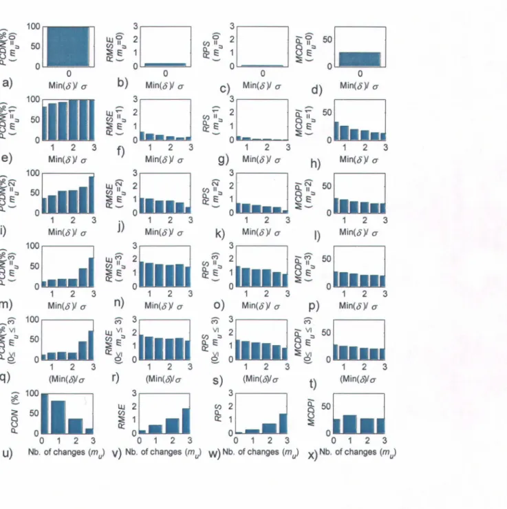
compiled as a function of the number of real changepoints and the minimum magnitude of the change in a given series. Similar results were compiled for the third simulated data set, but only using the number of changepoints since the series contained two kinds of changes with different definitions of the magnitude. These results are summarized in Tables 1 and 2 (resp. Tables 3 and 4) and plotted in Figure 1 (resp. Figure 2) for the first (resp. second) simulated data set. The same results are presented in Table 5 and Figure 3 for the third simulated data set. Analysis of these results aUows drawing the foUowing conclusions:
a) The rate of false detection is very low since the PCDN is close to 100% when mu
=
0 (Figures la, lu, 2a, 2u and 3a). The PCDN is remains very high when there is only one real change mu=
1 (Figures 1 e, 2e) and, as expected, it increases when the minimum magnitude of the change increases. The same conclusions can be drawn from aU the other performance measures considering that a good forecast means smaU RMSE, RPS and MCDPlvalues.b) The performance indices (except the MC DPI) decrease with the number of changepoints (c.f. Figures 1 and 2);
c) It seems easier for the method to detect shifts than changes in trend (Figure 1 vs Figure 2), although the relative performance depends on the range of change of magnitude in each set. This conclusion holds only if we consider that the range of magnitudes that were generated is representative of the real world.
Results suggest that in this particular case (series of 75 years) the method can be trusted if the shifts in the data set have the order of magnitude of the standard deviation, and if the number of changes is known to be inferior to three. Indeed, the performance should not be the same for other data sets with different lengths and different statistical characteristics. However, since the data
sets were generated to cover the range of magnitudes generally encountered in streamflow records, the method proposed in this paper will be useful for detecting changes in river discharges. It can also be used in several other problems involving multivariate linear regression, such as data homogenization or signal processing.
8. Application to cases studies
The methodology is applied herein to two case studies to illustrate its behaviour on real data and to compare it to the approach of Asse/in and Ouarda [2005]. The first case study deals with change detection in the linear regression describing the relationship between Summer-Autumn flood peaks and precipitations on the Broadback River basin. Seidou and Ouarda [2005] studied this data set using the Bayesian single changepoint detection method of Asselin and Ouarda [2005] and found that the relation has significantly changed after 1972 (Tc
=
1972). As in their paper, the changepoint Tc corresponds to the last point on the segment before the change and differs from the definition that was used in this paper (first point of the segment after the change), the expected value of T with the approach proposed in this paper should be 1973.The second case study is an example drawn from the Canadian Reference Hydrometrie Basin Network (RBHN) data base [Brimley et al., 1999]. The case was selected because it displayed a relatively large number of changes.
8.1. Changepoint detection in the finear regression describing the relationship befween Summer-Autumn flood peaks and precipitations on the Broadback River basin
8.1.1. The data
The Broadback River has a catchment of 17100 km2 and experiences forest fire bursts from time to time (Figure 4). According to the Canadian Large Fire Database [Stocks et al., 2002; Natural
Resources Canada, 2005], major forest fires occurred during the summer of 1971, buming 506
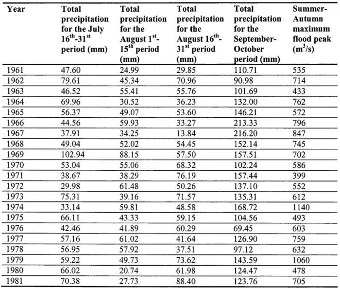
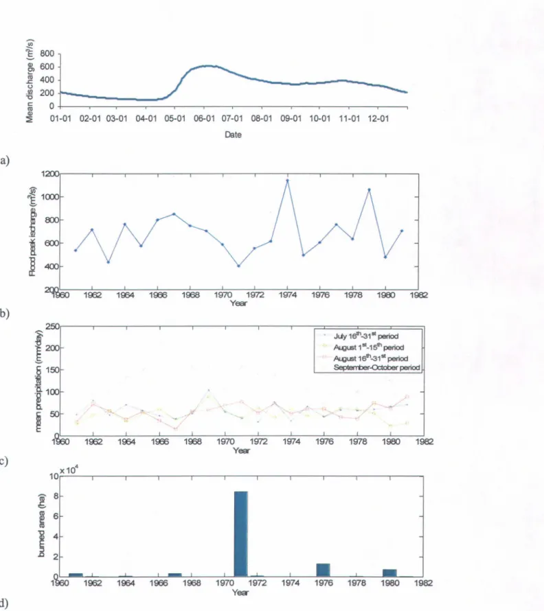
km2 in the upper parts of the catchment (1/34 of the total basin area). It can be hypothesized that the deforestation due to these fires can change the basin response function to meteorological inputs. In order to perform the analysis, the 1961-1981 daily flood discharges at station 80801 were obtained from Quebec Ministry of the Environment. The Broadback River is subject to two types of floods: spring floods, which are dominated by snowmelt, and summer-autumn floods which are caused by direct liquid precipitations. Figure 5a presents the mean daily discharge at this station for the 1961-1981 period. It appears that the summer-autumn maximum flood peak is generally observed at the end of October (Figure 5a). Daily precipitations for the July-October period from 1961 to 1981 were obtained by interpolation from the neighbouring weather stations on a regularly spaced grid of 100* 100 points and averaged to have a time series representing precipitation at the catchment scale. This time series was then used to ob tain the mean precipitation on the Broadback river catchment for every halfmonth period from July to October. Exploratory analysis of the linear relationship between observed flood discharge and the obtained precipitation series led to the choice of four explanatory variables for the flood peak values: 1) the mean precipitations of the 16th -31 st of July period, 2) the sum of precipitations of the 1 st_15th of August period, 3) the sum of precipitations of the 16th -31 st of August period and 4) total precipitations for the September-October period. The values of the 1961-1981 summer-autumn flood peaks are presented in Figure 5b and those of the chosen explanatory variables in Figure 5c. Figure 5d presents the bumed areas on the catchment for each year of the period of study. The series of explanatory variables as weIl as the maximum flood peaks are summarized in Table 6.
8.1.2. Results
The application of the changepoint detection method leads to a probability of 0.2 for the absence of changepoints and 0.8 for the existence of a unique changepoint (Figure 6a). A small weight «0.01) is attributed to the existence oftwo changes. The posterior probability distribution of the changepoint , is illustrated in Figure 6b. The posterior probability distribution of
'c
obtained with the same data set by Seidou and Ouarda [2005] with the Bayesian method of Asselin and Ouarda [2005] is also presented in Figure 6c. The two methods agree that the changepoint occurred probably between 1973 and 1974, with however different weights for these two dates. The weight differences may be due to the differences in the prior specifications of the two methods, and to the uncertainty introduced by the use of limited samples when computing the posterior distribution with the two approaches.8.2. Shifts and trend change detection in the flood peaks of the Ogoki river 8.2.1. The data
The Ogoki River is a 480 km long river located in the province of Ontario, Canada. It flows northeast from lakes west of Lake Nipigon to join the Albany River which ends into the James Bay. Station 04GB004 (Ogoki River above Whiteclay Lake) is part of the Canadian Reference Hydrometric Basin Network (RHBN) which comprises stations that have been carefully selected for climate change detection and assessment studies [Brimley et al., 1999]. The RHBN network comprises stations that are pristine. Station 04GB004 was selected because it displays a relatively large number of changepoints. The location of this station is given in Figure 7.
8.2.2. Results
The results of the changepoint analysis of the Ogoki River streamflows with the method proposed in this paper are presented in Figure 8. The results obtained with the approach of Asselin and Ouarda [2005] are provided in Figure 9. The posterior probability distribution of the number of changepoints obtained with the proposed method is plotted in figure 8a. Up to 4 changepoints are plausible (Pr(m
=
4) > 0), but the most probable number of changepoints is two. Figures 8b and 8c provide the posterior probability distributions of the first and second changepoints, conditional to m=
2 . The position of each of these changepoints is chosen to be the mode of the posterior distribution: 1961 for the first changepoint and 1971 for the second changepoint. Given these positions, the posterior means of the three segments in the data series are readily computed (Figure 8d). According to the analysis, the flows of the Ogoki River displayed a negative downward trend from 1951 to 1961, and increased regularly from 1960 to 1970. From 1960 to the present date, the streamflow record displayed a small downward trend.Figure 9a illustrates the posterior probability distribution of the changepoint obtained with the methodology of Asselin and Ouarda [2005]. This method gives less than 0.01 probability of no change (with this method, the probability of no change is equal to the probability that the changepoint is at the end of the data series). The mode of the posterior distribution of the date of change corresponds to 1967. This date corresponds grossly to the mean of the two changepoints detected with the methodology presented in this paper. This indicates that the results of the two methods are consistent. Although the method of Asselin and Ouarda [2005] is designed to detect only one change, a multimodal posterior distribution is often the sign of the existence of more than one changepoint. In this example, the fact that the posterior distribution is bimodal suggests
that there may be another changepoint in 1955. However, this seems to have been caused rather by the high discharge observed in 1954 than by a real change of trend in the data series.
Since the causes of trend change in the streamflow record are not known, it is impossible to decide whether the results of one or the other of the two methods correspond to the reality. The main advantage of the proposed approach is that it has less constraints and gives a larger chance for the data to influence the posterior distributions. The proposed approach is thus preferable in cases where there is only one response variable, where no data is missing and where more than one change is plausible. The results presented in this work are also easier to interpret than those of the approach proposed by Asselin and Ouarda [2005]
9. Conclusions and recommendations
A Bayesian method of multiple changepoint detection in multivariate linear regresslOn IS
developed and validated with both simulated data and real data sets. The paper also proposes a new c1ass of priors for the parameters of the multivariate linear model, as weIl as useful formulas that permit straightforward computation of the posterior distribution of the positions of changepoints. Results suggest that, in the particular case of series with 75 observations, the proposed method can be trusted if the shifts in the data set have the order of magnitude of the standard deviation, and if the number of changes is known to be inferior to three. It is also shown that in cases where there is only one response variable, where no data is missing and where more than one change is plausible, it is better to use the proposed methodology instead of Asselin and Ouarda [2005].
The extension of the work presented in this paper to much more general models is straightforward since the most important equations were obtained without assumptions on model structure. An
chain Models. Much more complex changepoint problems can be handled in the framework of hidden Markov chain models, especially those which display seriaI dependence structure in the observations [e.g Thyer and Kuczera, 2003a,b].
10. Acknowledgements
The financial support provided by the Natural Sciences and Engineering Research Council of Canada (NSERC), and the Nordic Study Center (CEN) is gratefully acknowledged. The authors are also grateful to the Quebec Ministry of the Environment for having provided the data sets used in the case studies.
List of symbols
1)/
Regression parameters before the changepoint in the methodology of Asselin and Ouarda [2005]
Regression parameters after the changepoint in the methodology of Asselin and Ouarda [2005]
Component of the vector of regression parameter that do es not change in the methodology of Asselin and Ouarda [2005]
Component of the vector of regression parameter that change to
P2
after Tc t in the methodology of Asselin and Ouarda [2005]Component of the vector ofregression parameter that change replaces
P
2 afterTc in the methodology of Asselin and Ouarda [2005]Vector of random errors in the linear regression equation (one response variable)
Part of the vector of random errors between s and t
Vector of random errors in the linear regression equation (several response variables)
Parameters of the linear regression equation
Variance-covariance matrix of the distribution of 1)/
Last point of the segment before the change (methodology of Asselin and Ouarda [2005])
kth changepoint in the proposed methodology Vector of regression parameters
Vector of regression parameters at date t given Tc (methodology of Asselin and Ouarda [2005])
c
d·
d·
o d' 1 E G(t) g(t) M MCDPI n N P(t,s), s '? t PCDN Q(t) r RMSE RPS uParameter of the prior distribution of <l> Number of explanatory variables
Number of explanatory variables for which the regression coefficients do not change
Number of explanatory variables for which the regression
coefficients display a change (methodology of Asselin and Ouarda [2005])
Set of generated scatter schemes
Cumulative probability distribution of the time interval between consecutive changepoints
Probability distribution of the time interval between consecutive changepoints
Cumulative probability distribution of the first changepoint Probability distribution of the first changepoint
Number of generated scatter schemes
Sk
=
gk ,l2k , ... ,l;k}
in the inference procedureNumber of scatter schemes to generate with the posterior distributions of the positions of changepoints
Multiple Change Detection Performance Index number of changes in the uth generated series
Estimate of the number of changes in the uth generated series Number of changes in the kth generated scatter scheme during the simulation of the changepoints
Length of the data series Number of sets to generate
Probability that t and s be in the same segment.
Percentage of Correct Detections of the Number of changepoints Likelihood of the segment Yt:n given a changepoint at t-1
Number ofresponse variables (methodology of Asselin and Ouarda [2005])
Root Mean Square Error Ranked Probability Score
kth scatter scheme generated with the posterior distributions ofthe positions of changepoints
Time
Estimate of the ith change in the kth generated scatter scheme
ith change in the kth generated Scatter scheme
Number of the generated series
{y}
u in the validation procedureVector of explanatory variables
lh
row of the vector of explanatory variables Rows t to s of the vector of explanatory variablesReferences
Rows t to s of the vector of response variables uth generated series in the validation procedure
Asselin, J.J, Ouarda, T.B.M.J. (2005). Bayesian Multivariate Linear Regression with Application to Changepoint Models in Hydrometeorological Variables. Part 1. Model Development. Submitted to Water Resources Research.
Barry, D., and Hartigan, J. A (1992). Product Partition Models for Change Point Models. The Annals ofStatistics 20:260-279.
Barry, D., and Hartigan, J. A (1993). A Bayesian Analysis for Change Point Problems. Journal of the American Statistical Association 88: 3 09-319.
Beaulieu,
c.,
Ouarda, T.B.M.J. and Seidou, O. (2005). Comparative study of homogenization techniques for precipitation data series (in French). Progress report No 3 (Project on the homogenization of precipitation data). Ouranos Consortium, Montreal.Beibel, M. (1997). Sequential change-point detection in continuous time when the post-change drift is unknown. Bernoulli Journal of Mathematical Statistics and Probability 3(4): 457-478
Booth, N.B. and Smith, AF.M. (1982). A Bayesian approach to retrospective identification of change-points. Journal of Econometrics 19 :7-22.
Brimley, B., Cantin, J.F., Harvey, D., Kowalchuk, M., Marsh, P., Ouarda, T.B.M.J., Phinney, B., Pilon, P., Renouf, M., Tassone, B., Wedel, R. and T. Yuzyk (1999). Establishment of the reference hydrometric basin network (RHBN). Research report, Environment Canada, 41p.
Bruneau, P. and Rassam, J.-C. (1983). Application d'un modèle bayésien de détection de changements de moyennes dans une se'rie. Journal des Sciences Hydrologiques 28: 341-354.
Buizza, R. and Palmer, T. N. (1998). Impact of Ensemble Size on Ensemble Prediction. Monthly Weather Review 126(9): 2503-2518.
Burn, D.H. and Hag Elnur, M.A (2002). Detection of hydrologic trends and variability. Journal ofhydrology 255: 107-122.
Daumer, M. and Falk, M. (1997). On-line detection (for state space models) using multi-process Kalman filters. Linear Aigebra and its applications 284: 125:135.
Easterling D.R. and Peterson T.C. (1992) Techniques for detecting and adjusting for artificial discontinuities in c1imatological time series: a review. Proc. of the Fifth International Meeting on Statistical Climatology, 22-26 June 1996, Toronto, Ontario, Canada.
Fearnhead. P. (2005). Exact and Efficient Bayesian inference for Multiple Changepoint Problems.
Preprints, online [http://www.maths.lancs.ac.uk/~feamheaIPScpt.ps].
Gelfand, A. E., Hills, S. E., Racine-Poon, A., and Smith, A. F. M. (1990). Illustration of Bayesian Inference in Normal Data Models Using Gibbs Sampling. Journal of the American Statistical Association ,85: 972-985.
Gut, A. and Steinebach, J. (2002). Truncated Sequential Change-point Detection Based on Renewal Counting Processes.Scandinavian Journal of Statistics 29(4):693-719.
Hamil, T.M. (2001). Interpretation of Rank Histograms for Verifying Ensemble Forecasts. Monthly Weather Review 129(3): 550-560.
Lai, T.L. (1995) Sequential change point detection in quality control and dynamical systems.
Journal of the Royal Statistical Society, (Serie B) 57:613-658
Lund, R. and Reeves, J. (2002) Detection ofundocumented changepoints: A revision of the two-phase regression model. Journal of Climate 15, 2547-2554.
Minka, P. (2001). Bayesian linear regression. Unpublished paper. Online [https:// research.microsoft.coml~minka/papers/minka-linear.ps.gz]
Moreno, E., Casella, G., and Garcia-Ferrer, A. (2005). An objective Bayesian analysis of the change point problem. Stochastic Environmental Research and Risk Assessment (SERRA) 19(3):191 - 204
Natural Resources Canada. (2005). Canadian Large Fires Database. Online document [http://fire.cfs.nrcan.gc.ca/Downloads/LFDB/LFD_5999_ e.ZIP]. downloaded on August 2005.
Perreault, L., Bernier, J., Bobée, B., and Parent, E. (2000a). Bayesian change-point analysis in hydrometeorological time series 1. Part 1. The normal model revisited. J of Hydrology
235: 221-241.
Perreault, L., Bernier, J., Bobée, B., and Parent, E. (2000b). Bayesian change-point analysis in hydrometeorological time series 2. Part 2. Comparison of change-point models and forecasting. Journal of Hydrology 235: 242-263.
Perreault, L., Haché, M., Slivitzky, M., and Bobée, B. (1999). Detection of changes in precipitation and runoff over eastern Canada and D.S. using a Bayesian approach.
Stochastic Environmental Research and Risk Assessment 13:201-216.
Perreault, L., Parent, É., Bernier, J., and Bobée, B. (2000c). Retrospective multivariate Bayesian change-point analysis: A simultaneous single change in the mean of several hydrological sequences. Stochastic Environmental Research and RiskAssessment,14: 243-261.
Salinger, M. (2005). Climate Variability and Change: Past, Present and Future - An Overview. Climatic Change 70: 9-29
Seidou, O., Ouarda, T.B.M.J. (2005). Bayesian Multivariate Linear Regression with Application to Changepoint Models in Hydrometeorological Variables. Part II. Cases studies. Submitted to Water Resources Research.
Stephens, D. A. (1994). Bayesian Retrospective Multiple-changepoint Identification. Applied Statistics 43: 159-178.
Solow, A.R. (1987). Testing for c1imate change: an application of the two-phase regression mode!. Journal of Applied Meteorology 26, 1401-1405.
Stocks, B.J.; Mason, J.A.; Todd, J.B.; Bosch, E.M.; Wotton, B.M.; Arniro, B.D.; Flannigan, M.D.;Hirsch, K.G.; Logan, K.A.; Martell, D.L.and Skinner, W.R. (2002). Large forest fires in Canada, 1959-1997. Journal of Geophysical Research (107,8149,doi:1O.1029/2001 JD000484).
Thyer, M and Kuczera, G. (2003a). A hidden Markov model for modelling long-term persistence in multi-site rainfall time series 1. Model calibration using a Bayesian approach. Journal ofHydrology 275:12-26
Thyer, M and Kuczera, G. (2003b). A hidden Markov model for modelling long-term persistence in multi-site rainfall time series. 2. Real data analysis. Journal of Hydrology 275:27-48. Vincent, L.A. (1998). A technique for the identification of inhomogeneities in Canadian
temperature series. Journal of climate Climate Il, 1094-1105.
Wang, x.L. (2003). Comments on 'Detection ofUndocumented Changepoints: A revision of the Two-Phase regression mode!'. Journal of Climate 16, 3383-3385.
West, M. (1984). Outlier models and prior distributions in Bayesian linear regression. Journal of the Royal Statistical Society (Ser. B), 46: 431-439
Woo, M. and Thome, R. (2003). Comment on 'Detection ofhydrologic trends and variability' by Bum, D.H. and Hag Elnur, M.A., 2002. Journal of Hydrology 255, 107-122. Journal of hydrology 277:150-160.
Yao, y. (1984). Estimation of a noisy discrete-time step function: Bayes and empirical Bayes approaches. The Annals ofStatistics 12: 1434:1447
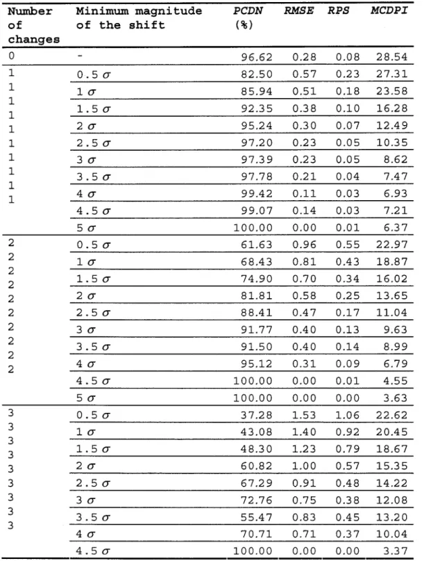
Table 1 : Performance of the changepoint detection procedure as function of the number of real changepoints and the minimum magnitude of the shift for the first simulated set.
Nwnber Minimum magnitude PCDN RMSE RPS MCDPI
of of the shift (%) changes 0 96.62 0.28 0.08 28.54 1 0.50- 82.50 0.57 0.23 27.31 1 10- 85.94 0.51 0.18 23.58 1 1 1.50- 92.35 0.38 0.10 16.28 1 20- 95.24 0.30 0.07 12.49 1 2.50- 97.20 0.23 0.05 10.35 1 30- 97.39 0.23 0.05 8.62 1 3.50- 97.78 0.21 0.04 7.47 1 1 40- 99.42 0.11 0.03 6.93 4.50- 99.07 0.14 0.03 7.21 50- 100.00 0.00 0.01 6.37 2 0.50- 61.63 0.96 0.55 22.97 2 10-68.43 0.81 0.43 18.87 2 2 1. 5 0- 74.90 0.70 0.34 16.02 2 20- 81.81 0.58 0.25 13.65 2 2.50- 88.41 0.47 0.17 11.04 2 30- 91.77 0.40 0.13 9.63 2 3.50- 91.50 0.40 0.14 8.99 2 2 40- 95.12 0.31 0.09 6.79 4.50- 100.00 0.00 0.01 4.55 50- 100.00 0.00 0.00 3.63 3 0.50- 37.28 1.53 1.06 22.62 3 10- 43.08 1.40 0.92 20.45 3 3 1.50- 48.30 1.23 0.79 18.67 3 20- 60.82 1.00 0.57 15.35 3 2.50- 67.29 0.91 0.48 14.22 3 30- 72.76 0.75 0.38 12.08 3 3.50- 55.47 0.83 0.45 13.20 3 40- 70.71 0.71 0.37 10.04 4.50- 100.00 0.00 0.00 3.37
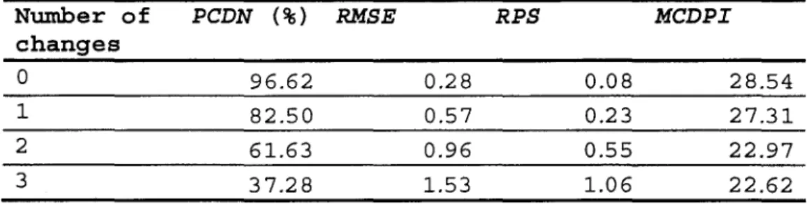
Table 2 : Performance of the changepoint detection procedure as function of the number of real changepoints for the first simulated set.
Number of PCDN (%) RMSE RPS MCDPI
changes
0 96.62 0.28 0.08 28.54
1 82.50 0.57 0.23 27.31
2 6l.63 0.96 0.55 22.97
Table 3: Performance of the changepoint detection procedure as function of the number of real changepoints and the minimum magnitude of the shift for the second simulated set. Number Minimum magnitude of PCDN RMSE RPS MCDPI
of the trend (per ten (%) changes epochs) 0 97.33 0.23 0.06 27.03 1 0.5 a 80.71 0.59 0.26 33.56 1 l a 88.95 0.46 0.15 25.86 1 1 1.5 a 93.42 0.36 0.09 20.38 1 20' 96.80 0.25 0.06 16.97 1 2.5 a 98.13 0.19 0.05 13.42 30' 97.65 0.22 0.04 12.31 2 0.5 a 36.59 1.10 0.74 28.03 2 l a 42.64 1.04 0.65 25.22 2 2 1.50' 54.29 0.93 0.54 21.80 2 20' 56.11 0.89 0.49 19.78 2 2.5 a 63.96 0.77 0.40 17.56 30' 91.29 0.41 0.19 17.27 3 0.5 a 12.57 1.82 1.47 27.27 3 l a 16.55 1.71 1.35 25.80 3 3 1.5 a 18.79 1.61 1.26 23.64 3 20' 17.96 1.56 1.21 21.60 3 2.5 a 44.72 1.61 1.04 20.78 30' 70.71 1.41 0.88 20.41
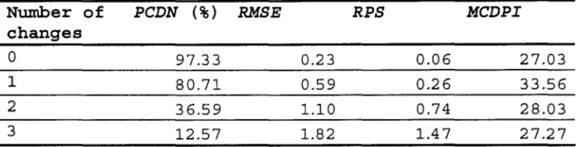
Table 4 : Performance of the changepoint detection procedure as function of the number of real changepoints for the second simulated set.
Nwnber of PCDN (%) RMSE RPS MCDPI
changes
0 97.33 0.23 0.06 27.03
1 80.71 0.59 0.26 33.56
2 36.59 1.10 0.74 28.03
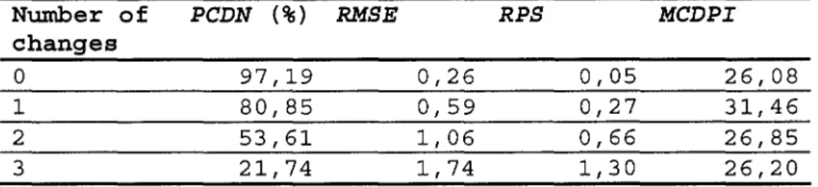
Table 5 : Performance of the changepoint detection procedure as function of the number of real changepoints for the third simulated set.
Number of PCDN (%) RMSE RPS MCDPI
changes
0 97,19 0,26 0,05 26,08
1 80,85 0,59 0,27 31,46
2 53,61 1,06 0,66 26,85
Table 6: Basin scale precipitation and summer-autumn flood peak time series for the Broadback river basin.
Year Total Total Total Total
Summer-precipitation precipitation precipitation precipitation Autumn
for the July for the for the for the maximum
16th_31st August 1st_ August 16th_ September- flood peak period (mm) 1Sth period 31st period October (m3/s)
(mm) (mm) (!eriod ~mm) 1961 47.60 24.99 29.85 110.71 535 1962 79.61 45.34 70.96 90.98 714 1963 46.52 55.41 55.76 101.69 433 1964 69.96 30.52 36.23 132.00 762 1965 56.37 49.07 53.60 146.21 572 1966 44.56 59.93 33.27 213.33 796 1967 37.91 34.25 13.84 216.20 847 1968 49.04 52.02 54.45 152.14 745 1969 102.94 88.15 57.50 157.51 702 1970 53.04 55.06 68.32 102.24 586 1971 38.67 38.29 76.19 157.44 399 1972 29.98 61.48 50.26 137.10 552 1973 75.31 39.16 71.57 135.31 612 1974 33.14 59.81 48.58 168.72 1140 1975 66.11 43.33 59.15 104.56 493 1976 42.46 41.89 60.29 69.45 603 1977 57.16 61.02 41.64 126.90 759 1978 56.95 57.92 37.51 97.12 632 1979 59.22 49.73 73.62 143.59 1060 1980 66.02 20.74 61.98 124.47 478 1981 70.38 27.73 88.40 123.76 705
FIGURES CAPTION
Figure 1: Perfonnance of the changepoint detection procedure as function of the number of real changepoints and the minimum magnitude of the shift for the first simulated set. ... 36 Figure 2: Perfonnance of the changepoint detection procedure as function of number of real
changepoints and the minimum magnitude of the shift for the second simulated set. ... 37 Figure 3: Perfonnance of the changepoint detection procedure as function of the number of
real changepoints for the third simulated set. ... 38 Figure 4: Location map of station 080801 (broadback River) ... 39 Figure 5: Data for changepoint detection in summer-auturnn flood peaks for the Broadback
river: a) mean hydrograph; b) summer-auturnn flood peak time series; c) precipitation time series; d) bumed catchment area time series ... 40 Figure 6 : Changepoint detection in summer-auturnn flood peaks of the Broadback river: a)
posterior probability of the number of changepoints; b) posterior probability of the first point of the segment after the changepoint obtained with the proposed methodology; c) posterior probability of the last point of the segment before the change obtained with the methodology of Asselin and Ouarda [2005]; ... 41 Figure 7: Location of station 04GB004 (Ogoki River above Whitec1ay Lake) ... .42 Figure 8: detection of trend changes at station 04GB004 (Ogoki River above Whitec1ay
Lake) with the proposed methodology ... 43 Figure 9: detection of trend changes at station 04GB004 (Ogoki River above Whitec1ay
:;S!.~ o 0 ~II Q '" ü E a..~ a) e)
o
Min(o)/ a 2 4 Min(c5)/ a 100r----(J?C\i ~II Q '"50
ü E a.. ~ 0 i) m) 2 4 Min(c5)/ a 2 4 Min(c5)/ a ~ c;) 100 r - - - ---.n '# VI ~'" 50
QE~~
0 q) 2 4 (Min(b)/a~100
~
8
50
a.. 0o
1 2 3 U) Nb. of changes (mu)UJ'l?
(/)'"
~~ : 31
D
o
b) Min(c5)/ a~~'~
D
2 4 f) Min(c5)/ a UJ~ ~'"
i'i~ j) n) r) : 31
D
2 4 Min(c5)/ a~
~
2 4 Min(c5)/ a~
~
2 4 (Min(b)/a~~
o
CJ
1 2 3 V) Nb. of changes (mu) Ô (/)11 a.. '" a::~ c) ... (/)11 a.. '" a::~ g) N (/)11 a.. '" a::~ k) c;) (/)11 a.. '" a::~ 0) s)~D
o
Min(c5)/ a~D
2 4 Min(c5)/ a~
D
2 4 Min(c5)/ a Min(c5)/ a~
D
2 4 (Min(b)/a&~
D
Q'l?
50
[;;]
8
E'" ~~ 0o
d) Min(c5)/ aQ17 50
D
Q '" üE ~~ 0 2 4 h) Min(c5)/ aQ~50
D
Q '" üE ~~ 0 2 4 1) Min(c5)/ a p) Min(c5)/ aQ~I
50
D
Q ",,'" ü'" ~8 0 ~ 2 4 t) (Min(b)/a~50
~~
o
o
1 2 3 w) Nb. of changes (mu)o
1 2 3 X) Nb. of changes (mu)Figure 1: Performance of the changepoint detection procedure as function of the number of real changepoints and the minimum magnitude of the shift for the first simulated set.
100 '#.s ::!II a '" 50 ü E o..~
o
a) Min(,,)/o
a 100_ 50o
1 2 3 e) Min(,,)/ a'~
~
1 2 3 g) Min(,,)/ a h)~
~
~~'" ~
D
~~'" 50
~
1 0:':" 1 üEo
O:E~ 0 Min(,,)/ a Min(,,)/ a 1 2 3 1 2 3 1 2 3 i) j)'~
O
~~.~
~
&i:~
~
~}'):
a
m) 1 2 3 1 2 3 1 2 3 1 2 3Min(,,)/ a n) Min(,,)/ a 0) Min(,,)/ a p) Min(,,)/ a
'::
~
~;.:
CJ
~~,
r
-
i
~~
5011
O
~
o:~
0-0:~1 O
~
:E~I
01 l t W1 2 3 1 2 3 ~ 1 2 3 1 2 3
r) (Min(b)/ a s ) (Min(b)/ a t) (Min(b)/ a
~~
Q
&~
Q
~:
~
q) (Min(b)/a~
1001 L ]e.-S
50 0.. 0o
1 2 3 0 1 2 3 0 1 2 3 0 1 2 3u) Nb. of changes (mu) V) Nb. of changes (mu) w) Nb. of changes (mu) X) Nb. of changes (mu)
Figure 2: Performance of the changepoint detection procedure as function of number of real changepoints and the minimum magnitude of the shift for the second simulated set.
100 3 3 60 :$!. 2 2 !i!...- UJ CI) 0:: <: 50 CI) &:
8
408
~ ::lE Q.. 20o
o
2 3 00 2 3 1 2 3 00 1 2 3Nb. of changes (mu) Nb. of changes (m ) Nb. of changes (m )
a) b) u c) u d) Nb. of changes (mu)
Figure 3: Performance of the changepoint detection procedure as function of the number of real changepoints for the third simulated set.
STATION 080&01
/
4 · Location map Figure . 84. 2 don 916171 421 km bllrne don 20/6171 98 km2 burne:.=..,;_~ k River). . 080801 (broadbac of statIOna) b) c) d) .!!! ~ 400 _ _ _ - - - - _
i:~~b
~
i
20~
- - - -,-"'" : ,===
~ 01-01 02-01 03-01 04-01 05-01 06-01 07-01 08-01 09-01 10-01 11-01 12-01 Date 1~~--~----~--~----~--~----~--~----~--~----~--~ ~ 1962 1934 1~ 1968 1970 1972 1974 1976 1978 1900 1982 Year 1~ 1962 1934 1~ 1968 1970 1972 1974 1976 1978 1980 1982 Year 1962 1964 1~ 1968 1970 1972 1974 1982Yea-Figure 5: Data for changepoint detection in summer-autumn flood peaks for the Broadback river: a) me an hydrograph; b) summer-autumn flood peak time series; c) precipitation time series; d) burned catch ment area time series.
a) b) c) 2 0.7 , - - - r - - - , - - - r - - - - , - -- , -- - - - , - - . - - - , - - - . - - - , 1962 1964 1966 1968 1970 1972 1974 1976 1978 1980 '1 0.7, - -- , - - - r -- -, - - - r - - - - , - - - , - - - - , - - - - . - - - , - - - , 1962 1964 1966 1968 1970 1972 1974 1976 1978 1980
Yea-Figure 6 : Changepoint detection in summer-autumn flood peaks of the Broadback river: a) posterior probability of the number of changepoints; b) posterior probability of the first point of the segment after the changepoint obtained with the proposed methodology; c) posterior probability of the last point of the segment before the change obtained with the
00
40
30
~ _ _ ~ _ _ _ _ L -_ _ - L _ _ _ _ L -_ _ ~ _ _ ~ _ _ _ _ ~ _ _ ~ _ _ _-140 -130 -120 -110 -100 -00
-80
-70
-60
LorgitLde
1 , - - - - , - - - ,- - - -- -- - - -, -- - - -- - - - , - - - , , - - _ ,
"?
't::' 0.5 c.. a) 2 3 4 m~ :~~l
:
.~_
:
~II~:-_-_
:~
I
~, ~' :~'
l
b) ë\I' Il ..§. 1955 1960 1965 1970 1975 T 1 1980 1985 1990 1995 0.2.---,---~--~---,---.----.---,---~--~-, 0.1 \0.0'" c) O~--~--~~--~ --1955 1960 1965 1970 1975 1980 1985 1990 1995 T 2 6r-"----,----,---.----,---~==~====~===r~ ---*-Observed f10ws 5 - Simulated mean f10ws ~Mg
4 ' d) ~ 3 o q:: 2 \ 1L---~----L---~~--~----~----~----~----L---~~ 1955 1960 1965 1970 1975 1980 1985 1990 1995 YearsFigure 8: detection of trend changes at station 04GB004 (Ogoki River above Whiteclay Lake) with the proposed methodology.
0.4~~----~--~----~--~----~--~----~--~~ 0.3
-::-
u
'L::' 0.2 0... 0.1a)
5 ... If) C"')- 4 E-
If) ~ 3 o Li: 2 1955 1960 1965 1970 1975 1980 1985 1990 1995 Years . Observed flows- simulated mean flows
1 L-~L---~--~----~--~----~--~----~---L~
1955 1960 1965 1970 1975 1980 1985 1990 1995
b)
YearsFigure 9: detection of trend changes at station 04GB004 (Ogoki River above Whiteclay
Appendix 1: properties of p(er 1 a,e) oc er-a exp(--;-), a> 1,e > 0 2er
'"
Let I(a)
=
f er-a exp( --;-)dera=O 2er
a-3 I-a '" a-3 a-I 1 I(a)
=
22 e 2 f t(a-3)/2 exp ( -t)dt=
2--2 e -2 r(a; )a=O x [1.1 ] [1.2] [1.3] [1.4] [1.5] [1.6]
The case a < 3 leads to an infinite variance for er, i.e.
lim
fp(er)der=
+00. Any value of a lessX~+oO 0
than 3 can thus be used as a non informative prior. Note that when er is very large, p( er) oc er-a.
Appendix 2: Derivation of P(t,s)
In this section we will derive the expression for P(t,s). Let 00 be the ordinary least square solution of the equation YI:S