Source apportionment of submicron organic aerosols at an urban site by linear unmixing of aerosol mass spectra

HAL Id: hal-00302289

https://hal.archives-ouvertes.fr/hal-00302289

HAL is a multi-disciplinary open access

archive for the deposit and dissemination of sci-entific research documents, whether they are pub-lished or not. The documents may come from teaching and research institutions in France or abroad, or from public or private research centers.

L’archive ouverte pluridisciplinaire HAL, est destinée au dépôt et à la diffusion de documents scientifiques de niveau recherche, publiés ou non, émanant des établissements d’enseignement et de recherche français ou étrangers, des laboratoires publics ou privés.

Source apportionment of submicron organic aerosols at

an urban site by linear unmixing of aerosol mass spectra

V. A. Lanz, M. R. Alfarra, Urs Baltensperger, B. Buchmann, C. Hueglin,

André Prévôt

To cite this version:

V. A. Lanz, M. R. Alfarra, Urs Baltensperger, B. Buchmann, C. Hueglin, et al.. Source apportionment of submicron organic aerosols at an urban site by linear unmixing of aerosol mass spectra. Atmospheric Chemistry and Physics Discussions, European Geosciences Union, 2006, 6 (6), pp.11681-11725. �hal-00302289�

ACPD

Full Screen / Esc

Printer-friendly Version

Interactive Discussion

Atmos. Chem. Phys. Discuss., 6, 11681–11725, 2006 www.atmos-chem-phys-discuss.net/6/11681/2006/ © Author(s) 2006. This work is licensed

under a Creative Commons License.

Atmospheric Chemistry and Physics Discussions

Source apportionment of submicron

organic aerosols at an urban site by linear

unmixing of aerosol mass spectra

V. A. Lanz1, M. R. Alfarra2, U. Baltensperger2, B. Buchmann1, C. Hueglin1, and A. S. H. Pr ´ev ˆot2

1

Empa, Swiss Federal Laboratories for Materials Testing and Research, Laboratory for Air Pollution and Environmental Technology, 8600 Duebendorf, Switzerland

2

PSI, Paul Scherrer Institute, Laboratory for Atmospheric Chemistry, 5232 Villigen PSI, Switzerland

Received: 11 September 2006 – Accepted: 10 November 2006 – Published: 21 November 2006

Correspondence to: C. Hueglin (christoph.hueglin@empa.ch)

ACPD

Full Screen / Esc

Printer-friendly Version

Interactive Discussion Abstract

Submicron ambient aerosol was characterized in summer 2005 at an urban back-ground site in Zurich, Switzerland, during a three-week measurement campaign. Highly time-resolved samples of non-refractory aerosol components were analyzed with an Aerodyne aerosol mass spectrometer (AMS). Positive matrix factorization

5

(PMF) was used for the first time for AMS data to identify the main components of the total organic aerosol and their sources. The PMF retrieved factors were com-pared to measured reference mass spectra and were correlated with tracer species of the aerosol and gas phase measurements from collocated instruments. Six factors were found to explain virtually all variance in the data and could be assigned either

10

to sources or to aerosol components such as oxygenated organic aerosol (OOA). Our analysis suggests that at the measurement site only a small (<10%) fraction of organic

PM1originates from freshly emitted fossil fuel combustion. Other primary sources

iden-tified to be of similar or even higher importance are charbroiling (10–15%) and wood burning (∼10%), along with a minor source interpreted to be influenced by food cooking

15

(6%). The fraction of all identified primary sources is considered as primary organic aerosol (POA). This interpretation is supported by calculated ratios of the modelled POA and measured primary pollutants such as elemental carbon (EC), NOx, and CO,

which are in good agreement to literature values. A high fraction (60–69%) of the mea-sured organic aerosol mass is OOA which is interpreted mostly as secondary organic

20

aerosol (SOA). This oxygenated organic aerosol can be separated into a highly aged fraction, OOA I, (40–50%) with low volatility and a mass spectrum similar to fulvic acid, and a more volatile and probably less processed fraction, OOA II (on average 20%). This is the first publication of a multiple component analysis technique to AMS organic spectral data and also the first report of the OOA II component.

25

ACPD

Full Screen / Esc

Printer-friendly Version

Interactive Discussion 1 Introduction

Ambient aerosols have several adverse effects on human health (Nel, 2005), atmo-spheric visibility (Horvath, 1993) and a more uncertain impact on climate forcing (Lohmann and Feichter, 2005; Kanakidou et al., 2005). The organic component of atmospheric aerosols plays an important role mainly concerning small particles: at

Eu-5

ropean continental mid-latitudes, a fraction of 20–50% of the total fine aerosol mass can be attributed to organic matter (Putaud et al., 2004), and about 70% of the organic carbon mass (suburban summer) is found in particles with an aerodynamic diameter of less than 1µm (Jaffrezo et al., 2005).

Particles in the atmosphere are often divided into two categories, depending on

10

whether they are directly emitted into the atmosphere or formed there by condensation (Fuzzi et al., 2006). Primary organic aerosol (POA) particles are generally understood to be those that are released directly from various sources. Secondary organic aerosol (SOA) is formed in the atmosphere by condensation of low vapour pressure products from the oxidation of organic gases. The quantification of different types of aerosols

15

such as SOA and POA (or more classes if possible) is important as source identifi-cation is the first step in all mitigation activities. Furthermore, SOA and POA may be associated with different sizes, chemical composition and physical properties and thus may have different effects on climate or health.

Different classes of aerosols also exhibit different local abundances. SOA is a

sig-20

nificant contributor to the total ambient aerosol loading on a global and regional level. The SOA contribution to organic aerosol (OA) is highly variable, according to mod-elling results ranging from 10% in Eastern Europe to 70% in Canada (Kanakidou et al., 2005). There is an ongoing debate about how much SOA is present in the urban tropo-sphere, where fresh emissions and aged air masses meet. As an example, Cabada et

25

al. (2004) advocate that in Pittsburgh 35% of the organic carbon is secondary in July, while one can deduce from another study that about 52% (calculated from Zhang et al., 2005b) of the organic aerosol mass was secondary in the same city in September.

ACPD

Full Screen / Esc

Printer-friendly Version

Interactive Discussion

Established approaches for SOA estimates are either based on VOC emission data (e.g. Jenkin et al., 2003), on the organic to elemental carbon (OC/EC) ratio in primary emissions (Turpin and Huntzicker, 1995; Cabada et al., 2004), or on mass spectral tracer deconvolution technique to separate hydrocarbon-like organic aerosol and oxy-genated organic aerosol (HOA and OOA) (Zhang et al., 2005a). “Algorithm 2” refers to

5

this latter technique and represents the first multivariate analysis of Aerodyne aerosol mass spectrometer (AMS) data.

In Algorithm 2, a priori knowledge of mass spectral data is incorporated into an alter-nating regression-like procedure (Paatero, 1994), when spectral markers m/z (mass-to-charge ratio) 44 and m/z 57 are set as first-guess principal components (in version 1.1

10

other mass tracers are suggested along with 44 and 57:http://www.asrc.cestm.albany. edu/qz/; in the future, a 4-factorial algorithm will be presented; Zhang et al., personal communication). Marker m/z 44 (a signal mainly from di- and poly-carboxylic acids functional groups, CO+₂) represents oxygenated organic aerosol components, while

m/z 57 (butyl, C4H+9) is a tracer for hydrocarbon-like combustion aerosol (e.g. diesel 15

exhaust). All reconstructed organic mass can be expressed as functions of m/z 44 and

m/z 57, which implies that all information of the 270-dimensional data (number of mass

fragments that contain information on organics out of a total of 300) can by explained by these two m/z. Algorithm 2 has been proven to reconstruct measured organics very well with OOA and HOA at three urban locations. Under carefully selected conditions,

20

OOA and HOA seem to be accurate estimates for SOA and POA, respectively (Zhang et al., 2005b; Volkamer, 2006). However, the presence of more than two active sources (likely in the urban troposphere) might limit the use of 2-factorial approaches.

In this paper, a method that allows the identification and attribution of more than two organic aerosol sources and components is presented. The apportionment of more

25

distinctive aerosol types and source classes allows for a more accurate modelling of SOA and POA. Our approach does not rely on chemical assumptions and is based on positive matrix factorization (PMF; Paatero and Tapper, 1994; Paatero, 1997). PMF has several advantages over common versions of factor analytical approaches based

ACPD

Full Screen / Esc

Printer-friendly Version

Interactive Discussion

on the correlation matrix as it will be discussed later. In atmospheric aerosol science, PMF has been successfully applied to deduce either sources of PM₁₀, the mass con-centration of particles with an aerodynamic diameter less than 10µm (Hedberg et al.,

2005; Yuan et al., 2006) or finer fractions of particulate matter such as PM2.5– (Polissar et al., 1998, 1999; Maykut et al., 2003; Kim et al., 2004; Kim and Hopke, 2005; Zhao

5

and Hopke, 2006; Pekney et al., 2006) or both (Kim et al, 2003; Begum et al., 2004; Chung et al., 2005). To our knowledge, no attempts have been made so far to apply PMF on submicron organic aerosol data. In most PMF studies, inorganic chemical species (mostly SO2−₄ and NO−₃) as well as trace elements were measured to describe the particulate composition of the aerosol phase. Organic components were studied

10

in less detail. Some PMF studies include EC and OC (Ramadan et al., 2000; Song et al., 2001; Liu et al., 2003). Zhao and Hopke (2006) distinguished four different OC and three different EC fractions depending on the thermal stability, as well as organic pyrolized carbon.

In the present study, 270 highly time-resolved organic fragments (mass-to-charge

15

ratios, m/z) retrieved from an Aerodyne AMS (Jayne et al., 2000; Jimenez et al., 2003) were analyzed with PMF. When the factors and scores that result from PMF calcula-tions are interpreted as aerosol sources and source strengths, respectively, it is nec-essary to verify these interpretations. Thus, the resulting scores were correlated with species that are indicative of primary (e.g. CO, NOx) and secondary (e.g. gaseous ox-20

idants, particulate nitrate and sulphate) components in the troposphere. It was further examined whether the calculated scores are capable to reproduce emission events of dominant aerosol sources that were observed during the sampling period. Moreover, the spectral similarity of the PMF calculated factors and AMS reference spectra was evaluated. Finally, the variances in generally accepted marker m/z’s (e.g. m/z 44 for

25

oxidized aerosol spectra) that can be explained by the resulting factor, EV(F) (Paatero, 2000), were inspected.

ACPD

Full Screen / Esc

Printer-friendly Version

Interactive Discussion

2 Measurements

The site of Zurich-Kaserne represents an urban background location in the centre of a metropolitan area of about one million inhabitants. The sampling site is at a public backyard, adjacent to a district with a high density of restaurants (West) and about 500 m from the main train station (Northeast). An Aerodyne AMS with a quadrupole mass

5

spectrometer was deployed during three weeks in summer 2005 (from 14 July to 4 Au-gust). A detailed description of the AMS measurement principles (Jayne et al., 2000) its modes of operation (Jimenez et al., 2003) and data analysis (Alfarra et al., 2004; Allan et al., 2003, 2004) are provided elsewhere. Meteorological parameters and trace gases were measured with conventional instruments by the Swiss National Air Pollution

10

Monitoring Network, NABEL (Empa, 2005): ten minute mean values of nitrogen oxides (NOx) were measured using chemiluminescence instruments with molybdenum

con-verters (APNA 360, Horiba, Kyoto, Japan), a non-dispersive infrared (NDIR) technique was used to determine carbon monoxide (CO) (APMA 360, Horiba, Kyoto, Japan), and ozone was determined by UV absorption (TEI 49C, Thermo Electron Corp., Waltham,

15

MA). Hourly organic carbon (OC) and elemental carbon (EC) data was retrieved from a semi-continuous EC/OC analyser (Sunset Laboratory Inc., Tigard, OR).

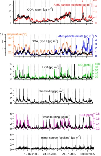
The sampling period is characterized by two phases of elevated photochemical ac-tivity – indicated by high temperatures – each followed by rainfall (Fig. 1). Fireworks on the Swiss national holiday (night of 1 August) are included. Nearby log-fires,

charbroil-20

ing events and delivery vans caused other isolated peaks of organic aerosol (Fig. 1). A total number of about 15 000 mass spectra (MS) were acquired (averaging time = 2 min). These MS are defined by vectors of 300 elements (m/z’s). 270 elements contain reliable information about the organic aerosol phase (m/z 12–13, 15–20, 24– 27, 29–31, 37–38, 41–45, 48–148, 150–181, 185, and 187–300). The other m/z’s

25

were excluded due to dominant contributions of the air signals (e.g. m/z 28, 32 and 40 for N2, O2 and Ar, respectively), inorganic species (e.g. m/z 39 and 46 for K and

nitrate, respectively), high background levels (e.g. m/z 186) or lack of plausible organic

ACPD

Full Screen / Esc

Printer-friendly Version

Interactive Discussion

fragments (e.g. m/z<12). For more details on the interpretation of organic fragments

see Allan et al. (2004) and Zhang et al. (2005a).

A collection efficiency (CE) value is required for the estimation of aerosol mass con-centration measured by the AMS (Alfarra et al., 2004). For the results reported in this study, a CE value of unity has been used. This CE value was validated for the total

5

AMS measured mass using data from a collocated beta-gauge instrument measuring a total PM₁₀ concentration. In addition, OC data was used to validate the CE value for the organic mass concentration.

3 Data analysis

Statistical analyses were carried out with the statistical software R version 2.1.1 (http:

10

//www.r-project.org, GNU GENERAL PUBLIC LICENSE Version 2, June 1991) and IGOR PRO 5.02 (Wavemetrics Inc., Lake Oswego, OR). Vectors (and matrices) are represented by (uppercase) bold letters. Single matrix elements as well as equations are written in lowercase italic letters.

3.1 Positive matrix factorization (PMF)

15

PMF is a well-established functional mixing model based on the work of Paatero and Tapper (1994) and Paatero (1997). The associated software “PMF2” (version 4.2) was used in this study. PMF is a receptor-only model and is most useful when source profiles are unknown. The fundamental principle of receptor modelling is that mass conservation can be assumed and a mass balance analysis can be used to identify and

20

apportion sources of airborne particulate matter in the atmosphere (Hopke, 2003). The most important advantages of PMF compared to common receptor models are that it is a least-squares algorithm taking data uncertainty into account and that its solutions are restricted to the non-negative subspace. Both features lay the foundation of making the link between the mathematical solution and the processes of the real world possible. In

25

ACPD

Full Screen / Esc

Printer-friendly Version

Interactive Discussion

practice, sources are better separated and positive scores and loadings are physically meaningful (Huang et al., 1999).

PMF is a factor analytical algorithm for linear un-mixing of data measured at a re-ceptor site. In PMF, the mass balance equation

X = GF (1)

5

is solved, with the measured data matrix, X, that combinest measurements (in time)

ofi variables (t×i matrix). The p rows of the F matrix (p×i matrix) are called factors

(or loadings), the columns of the t×p matrix G are called scores. The factors can

often be interpreted as emission source profiles, the corresponding source activity is then represented by the scores. However, the number of sources, p, that have an 10

impact on the data is typically unknown. Moreover, for a certain number of factorsp,

there is an infinite number of mathematically correct solutions to (1) given by rotated matrices G′=G T and F′=T−1 F (where the rotation matrix, T, multiplied by its inverse, T−1, equals the identity matrix). Most of these solutions are physically meaningless due to negativity. Therefore, PMF imposes non-negativity constraints to the unmixed

15

matrix elements. In this study, data matrix X consists ofi measured organic m/z’s at t

samples in time samples, ORG_ti. The matrix product of scores, G_tp, and factors, F_pi, defines the modelled organics, O ˆRG_ti.

X = ORGti = GtpFpi + Eti = O ˆRGti+ Eti (2)

where p is the number of factors (or remaining dimensions of the original 270-20

dimensional space) and E_ti the model error. Choosing the right number of factors or dimensions is a critical step in PMF. Often interpretability of G and F (along with diagnostic PMF values) is set as criterion for the optimump. This step requires a priori

knowledge and is highly subjective. Section 4.1 will be dedicated to this issue.

Factors G_tpand F_pi form an approximate bilinear decomposition of ORG_ti. This

fac-25

tor analysis problem is solved by minimizing the error, E_ti, weighted by measurement

ACPD

Full Screen / Esc

Printer-friendly Version

Interactive Discussion

uncertainty, S_ti, (weighted least square solved by a Gauss-Newton algorithm):

Q = arg min G minF X t X i ORG_ti− GtpFpi S_ti !2 , (3)

meaning that the value of the argument of the uncertainty weighted difference between the measured (ORG_ti) and modelled (G_tp F_pi) data matrix is at its minimum with re-spect to both fitting factors, the columns of G as well as the rows of F.

5

Thus, accurate uncertainty estimates of measured data are needed. Error estimates for a given AMS signal in [Hz]

S_ti = α s

(I_io+ Iib)

t_s (4)

were calculated from the ion signals m/z i, I_{i o}and I_ib (taking into account that the ion signal at blocked aerosol beam, I_{i b}, is subtracted from the open beam signal, I_io, in

10

order to calculate the ultimate AMS signal), sampling time, ts, and a statistical dis-tribution factor, α, and then transferred into organic-equivalent concentrations

(org-eq.µg m−3) using the IGOR PRO 5.02 code based on the work of Allan et al. (2003; http://cloudbase.phy.umist.ac.uk/people/allan/ja igor.htm). The organics data and un-certainty matrices, ORGti and Sti, were divided by the column median prior to PMF

15

analysis. Thus, similar absolute variances for every org_i are obtained and therefore also the low intensity m/z’s can provide important information in this analysis. PMF was run in the non-robust mode. Other parameters were set to default values and no data pre-treatment was performed.

3.2 Interpretation of factors and scores

20

For interpretation of the factors (rows of F) calculated by PMF, they were normalized and compared to measured reference spectra (Sects. 3.2.1 and 4.2). The correspond-ing scores (columns of G) were correlated with indicative marker species of sources

ACPD

Full Screen / Esc

Printer-friendly Version

Interactive Discussion

and atmospheric processes (Sect. 4.4). When factors are interpreted as source pro-files or aerosol components, they will be labelled with the name of the source or aerosol component. The corresponding scores are then called source activities.

3.2.1 Spectral similarity and reference spectra

The intensities of all obtained loadings (interpreted as mass spectra, msi) with

5

i=1. . . 300 m/z’s were first normalized

msnorm_i .= msi/X i

msi. (5)

The normalized spectra (msnorm_i .) were then correlated with normalized reference spectra from literature (msref_i .,norm.) and the coefficient of determination (R2) was cal-culated as a measure of spectral similarity. This approach however might have some

10

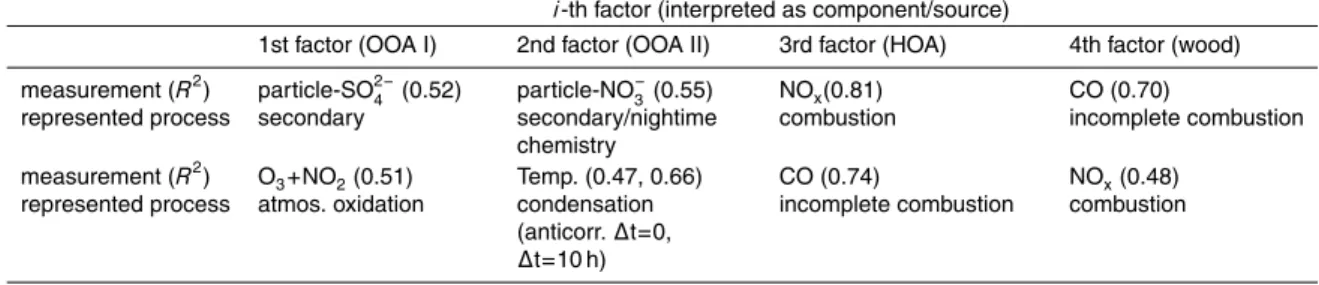
shortcomings when it is applied to AMS spectra, such as the leverage effect of a few, high intensity masses (e.g. m/z 18, 29, 43, 44) in regression analysis. These masses are typically small (m/z≤44). Therefore, spectral similarity was also calculated for m/z>44, R_m/z>442 , providing additional insight into the similarity of the low intensity masses only (values in parentheses; Table 1). The use of both values yields a more

15

robust assessment of similarity.

Reference spectra used for transformed OA include fulvic acid (Alfarra, 2004) as a tracer for highly aged particles, secondary organic aerosols from VOC precursors such asα-pinene, isoprene, 1,3,5-trimethylbenzene, m-xylene, and cyclopentene (Bahreini

et al., 2005; Alfarra et al., 2006a), as well as aged rural and urban aerosol from field

20

studies in Pittsburgh (Zhang et al., 2005a), Vancouver (Alfarra et al., 2004) and Manch-ester (Alfarra, 2004). At these places, spectra of freshly emitted combustion particles were determined, too. During several evenings of the sampling campaign at Zurich-Kaserne, charbroiling had been observed. To calculate the charbroiling reference spectra, the corresponding peaks were isolated and the background was subtracted.

25

Background was defined as the samples before and after the barbecue events that 11690

ACPD

Full Screen / Esc

Printer-friendly Version

Interactive Discussion

were within the same meteorological regime and without interference from other known special emission situations such as pure hydrocarbon plumes, fireworks on 1 August and others. Reference spectra for wood burning in the field were obtained by AMS measurements in Roveredo, Switzerland, where wood burning was found to be the dominant source of organic aerosol in winter-time (Alfarra et al., 2006b1). Additional

5

reference spectra for wood combustion were provided by the MS of the cellulose py-rolysis tracer levoglucosan (Schneider et al., 2006) and combustion of many different wood types (e.g. chestnut, oak, beech, spruce, Alfarra et al., 2006b1; Schneider et al., 2006). Canagaratna et al. (2004) performed chasing experiments of diesel vehicles in New York; in addition, spectra of pure diesel fuel and lubricant oil were obtained in the

10

lab. A comparison of our obtained spectra with an illustrative selection of the reference spectra is shown in Table 1. It contains the comparisons of all factors deduced from 2-to 7-fac2-torial PMF (n=27) with the selected reference spectra (n=11). This comparison is based on spectral similaritiesR2and R_m/z>442 (in brackets) as defined before. The most interesting results of this 594 element table will be discussed in detail later in

15

Sect. 4.2.

4 Results and discussion

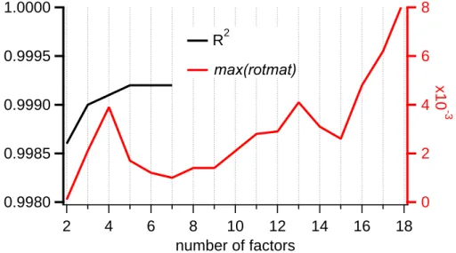
4.1 Determination of the number of factors

In PMF, choosing the number of factors often needs a compromise. Using too few fac-tors will coerce sources of different types into one factor, while using too many will split

20

real sources into unreal factors. PMF is a descriptive model and there is no objective criterion to choose the ideal solution. Interpretability as well as some PMF diagnostics (e.g. the rotational matrix, rotmat) is frequently used to determine the number of fac-tors. The PMF solutions for the data of Zurich-Kaserne were found to be very stable

1

Alfarra, M. R., Pr ´ev ˆot, A. S. H., Szidat, S., et al.: Identification of the mass spectral signature of organic aerosols from wood burning emissions, Environ. Sci. Technol., submitted, 2006b.

ACPD

Full Screen / Esc

Printer-friendly Version

Interactive Discussion

with respect to different ways of modelling the data uncertainty and other input options (e.g. EM, FPEAK, lims; Paatero, 2000) (data not shown). The largest element in

rot-mat, max(rotmat), is an estimate for the worst case rotational ambiguity (Lee et al.,

1999). A solution with rotational ambiguity means that the algorithm finds only vec-tor sets that are linear superpositions of the principal components. This represents

5

a mathematical drawback as the solution is not unique, i.e. the resolved factors can be rotated without changing the residuals associated with the model (rotational ambi-guity hampers the qualitative interpretation of the results). The PMF output rotmat is used here to detect the region of reasonable number of factors. There are three local minima in max(rotmat) versus number of factors shown in Fig. 2: one at two factors

10

(max(rotmat)=0.0001) and one at seven factors (max(rotmat)=0.0010). Values similar to the second minimum can be found from five to nine factors. The third local minimum is at 15 factors (max(rotmat)=0.0026), but uninterpretable factors (e.g. overwhelming dominance of m/z 15 or m/z 41) can be observed as soon as the number of sources is increased from seven to eight. These findings suggest that the 2- or 5- to 7-factorial

15

models are most promising to deduce the OA components and sources unambigu-ously. Therefore, we will study these in detail in the following. In Sect. 4.2 we describe what happens, when the number of factors is gradually increased from two to seven sources. In addition to rotmat, the fit of the regressed scores to measured organics for all PMF solutions was used for choosing the ideal number of factors,

20

or g_i = a +X p

b_pg_tp, (6)

A better fit is obtained by increasing the number of factors from two to five. In this case, a plateau is reached at five factors (R2=0.9992). Even with only two factors, already 99.86% of the variance of the measured organics can be explained by the model. Note that the intercept a is virtually zero and the overall slope is 1.00 for any PMF 25

model introduced. The productsb_pg_tp in Eq. (6) represent normalized scores and are estimates for the contributions of each source to total organics. They are shown for

p=6 as absolute values (Fig. 6) and as relative values (Fig. 4). This normalization is

ACPD

Full Screen / Esc

Printer-friendly Version

Interactive Discussion

most promising when the aim is to estimate accurate source contributions. However, it is important to note that the spectral similarity (Sects. 3.2.1 and 4.2), the correlation of scores with indicative species (Sect. 4.4) as well as the approximation of the data matrix (reconstructed organics as discussed in Sect. 3.1 and calculated in Sect. 4.3) are invariant to factor normalization.

5

4.2 Interpretation of factors and mass allocation

The source profiles and its activities will be discussed in order of decreasing explained variance, EV(F), as described in Paatero (2000). It is a measure of how important each factor is in explaining the variance in the m/z’s. The order of discussion is reflected in Table 1.

10

Each factor (or calculated MS) of the 6-factorial PMF is presented in Fig. 3. This figure shows the normalized intensity (according to Eq. 5) versus mass-to-charge ratio of all six factors retrieved from PMF. As specific calculated spectra (e.g. the factors interpreted as HOA) from different factorial approaches show less variability than a certain group of the reference spectra (e.g. all spectra referring to wood burning), the

15

selection of 6-factorial solutions is representative for the factors that are not shown here. It is the 6-factorial solution that includes the highest number of interpretable factors and we will proceed with when the discussion turns to source activities. In this section, the discussion includes all solutions of 2- to 7-factorial PMF analyses.

4.2.1 Two-factorial solution

20

Assuming two factors in PMF modelling, the first factor computed by PMF is most similar to OOA from Pittsburgh (R2=0.96), but also highly similar to all other OOA reference spectra obtained from field studies (R2>0.88). The second factor is closest to

the diesel fuel MS (R2=0.96), but also similar to the MS from chasing experiments and lubricant oil (R2>0.93). The average mass associated with the OOA-like factor is 87%, 25

while 13% are allocated to HOA (an overview of the average mass associated with each 11693

ACPD

Full Screen / Esc

Printer-friendly Version

Interactive Discussion

factor is summarized in Fig. 4.). The OOA factor as well as the HOA factor calculated by PMF are virtually identical (R2=0.99, R_m/z>442 =0.99 and R2=0.98, R_m/z>442 =0.99, respectively) to the corresponding factors calculated by using two first-guess principal components (m/z 44 and m/z 57).

4.2.2 Three-factorial solution

5

In the 3-factorial case, the first two factors generally exhibit more or less the same similarities to reference spectra as in the 2-factorial case. In fact, they are even slightly more similar to the spectra discussed above. The first factor is strongly correlated with secondary particles from Pittsburgh (R2=0.99) and the second factor has the highest correlation with the fuel reference MS (R2=0.98). The MS of the third factor is closely

10

related to charbroiling (R2=0.88). A mean mass percentage of 63% is attributed to OOA, 10% to HOA, and 27% to charbroiling-like aerosol. These changes compared to the 2-factorial model suggest that some primary particles (charbroiling and similar sources) are included in OOA, when assuming only two factors (see also Sect. 4.3). 4.2.3 Four-factorial solution

15

When a fourth factor is introduced, the first three factors do not change much in terms of similarity with reference spectra. The new fourth factor shows highest similarity to wood smoke from the Roveredo field measurements (R2=0.81). Using four factors, about 12% of the OA mass originates from wood burning-like aerosol. When the wood burning factor is introduced, modelled aerosol mass from charbroiling is reduced most

20

(difference between the mass attributed within the 3-factorial approach and the one within the 4 factorial approach: ∆mass=−7%).

ACPD

Full Screen / Esc

Printer-friendly Version

Interactive Discussion

4.2.4 Five-factorial solution

A dramatic change can be observed when five factors are used in PMF modelling: not as much in the change of max(rotmat) or the model fit (Sect. 4.1), but in terms of similarity to secondary aerosol. The original first, OOA-like factor is split into highly aged background aerosol (high similarity to aged rural aerosol: R2=0.97 and to fulvic

5

acid: R2=0.93) and one that mostly resembles aerosol from isoprene oxidation in the presence of NO_x (R2=0.82). We will refer to these OOA factors as “OOA, type I” and “OOA, type II”, respectively. The third spectrum is again associated with charbroiling (R2=0.82), the fourth with wood burning (similarity to Roveredo spectra: R2=0.70; levoglucosan: R2=0.71). Increasing the number of factors from four to five does not

10

affect the modelled mass of wood burning aerosol (∆mass=−2%) or fuel-like aerosol

(∆mass=−1%), while charbroiling aerosol again (∆mass=−6%) is loosing most of its

contribution. This indicates that using only three or four factors results in overestimating OA from charbroiling.

4.2.5 Six-factorial solution

15

With six factors, the first factor is even more similar to fulvic acid (R2=0.96), while the third factor is still very similar to fuel aerosol (R2=0.99). The second factor can be interpreted similarly as in the 5-factorial case. However, considering only m/z>44,

correlations are highest with α-pinene SOA rather than isoprene SOA. It should be

noted that in reality SOA from several precursors will contribute to this factor, where

20

the differences between the reference spectra do not seem to be significant enough to discriminate between those. The fourth factor can be interpreted as a charbroiling source again (R2=0.85), the fifth is even more levoglucosan-like (R2=0.82). The sixth factor does not fit in any class of reference spectra, but it might be associated with food cooking. The mass spectrum of this factor is characterised by m/z 264 with an intensity

25

of about 15% relative to the largest peak (m/z 43) and it is in the same range as m/z 60 in this factor. This might be an indication of oleic acid (NIST, 2006), the most abundant

ACPD

Full Screen / Esc

Printer-friendly Version

Interactive Discussion

monoenoic fatty acid in plant and animal tissues. However, Katrib et al. (2004) showed that m/z 264 is much more depleted in pure oleic acid than shown in this factor. There-fore, this is an indication that oleic acid might be lumped together with other similar fatty acids, such as petroselenic acid (which is present e.g. in coriander and parsley), pointing to food cooking as a partial source in that factor (additional evidence that this

5

factor might include food cooking aerosols will be given in Sect. 4.4.3). Going from five to six factors, the average mass does not change for fuel-like aerosols. In general, mass differences for all factors are small (|∆mass| ≤5%).

4.2.6 Seven-factorial solution

The first five factors in the 7-factorial solution are more or less the same as with six

10

factors. The seventh factor, tentatively assigned to food cooking, remains unchanged too, while the sixth factor does not correlate well with any of the available reference spectra: similarity is highest with the wood burning MS but correlations are lower than for the fifth factor. If the sixth factor is added to the fifth factor (interpreted as wood burning), the resulting factor exhibits increased correlation (R2=0.84, R_m/z>442 =0.87)

15

to ambient wood burning aerosols from Roveredo (but the same or lower correlation to other measured wood smoke spectra). This indicates that splitting real sources into un-real factors by assuming too many factors might already start at 7-factorial solutions to some extent. In addition, no more significant changes in the mass contribution to total organics take place, when we assume seven instead of six factors: charbroiling (10%)

20

and traffic-related fuel aerosol (6%) aerosol remain at constant levels, food cooking (∆mass=−1%) and OOA from local precursors (∆mass=+1%) are almost unchanged.

4.2.7 Evaluation of 2- to 7-factorial solutions

In summary, choosing only two factors in factor analytical models for this site overes-timates OOA if interpreted as SOA. At sites with two dominating sources this may be

25

ACPD

Full Screen / Esc

Printer-friendly Version

Interactive Discussion

less critical; as an example, Zhang et al. (2006)2 show that this OOA overestimation does not apply for the Pittsburgh dataset.

When three and more factors are assumed, aerosol from primary sources is sub-tracted from OOA and the first factor exhibits higher correlations with fulvic acid (which represents humic-like substances in the atmosphere; Gelencser, 2004).

5

The similarity of this first factor to fulvic acid is mainly increased when the number of factors is changed from two to three as well as from four to five. About 85–90% percent of the overall m/z 44 variance can be explained by this first factor. Evidence for m/z 44 and m/z 57 as tracers for oxygenated and hydrocarbon aerosol was first given in Alfarra et al. (2004).

10

A HOA-like factor is salient from 2- to 7-factorial PMF. The fraction of OA explained by HOA is decreasing from 13% in the 2-factorial approach to 6–7% in the 4- to 7-factorial approaches. The similarity to fuel is already strong when using only two fac-tors. Strongest similarity is reached when five factors are used. Most of the variance in the diesel marker m/z 57 can be explained by the HOA factor. In the 2-factorial case,

15

this amounts to 80% and monotonously decreases with each additional source down to about 50%. The wood burning-factor explains 12–13% of the m/z 57 variance.

When only three factors are chosen, wood burning is mainly lumped together with charbroiling (Sect. 4.2.3). Adding a fourth factor takes account of the fact that there is wood burning in summer (log-fires, barbecues, as well as domestic garden and forest

20

wood burning). At least four factors are necessary to identify wood burning. The factor identified as wood burning explains 45–55% of all variance in m/z 60. About 25% of

m/z 60 cannot be explained by the PMF models. About 25% of the m/z 73 variance is

explained by the charbroiling factor and nearly 20% by the wood burning factor, while 23% remain unexplained. Mass-to-charge ratio 60 and 73, as well as 137 have been

25

linked to wood burning by Schneider et al. (2006) as well as by Alfarra et al. (2006b)1.

2

Zhang, Q., Jimenez, J.-L., Dzepina, K., et al.: Component analysis of organic aerosols in urban, rural, and remote site atmospheres based on aerosol mass spectrometry, 7th Interna-tional Aerosol Conference, poster 5H8, St. Paul, Minnesota, USA, 2006.

ACPD

Full Screen / Esc

Printer-friendly Version

Interactive Discussion

The wood burning factor can account for 30–45% of the m/z 137 variance, and about 30% can not be explained by the model.

When a fifth factor is assumed, OOA is divided into highly aged background aerosol, which is fulvic acid-like and a second type that can not be clearly assigned to any reference MS (considering both,R2 and R_m/z>442 , see Table 1). Choosing five, six or

5

seven factors does not affect the solution significantly. Choosing more than seven fac-tors generates source profiles that cannot be interpreted. Changes from six to seven factors are very small. Additionally, the average mass associated with each source does not change much when we increase the number of factors from five to six factors, and even less when choosing seven instead of six factors (Fig. 4). With five factors, the

10

similarity plateau (defined byR2of 7-factorial solutions, which typically exhibit the high-est values) is not attained in most cases (Table 1), whereas the similarity to isoprene is highest with five factors. Therefore (and because of the findings from the 7-factorial solution, Sect. 4.2.6), using 6 factors might be a good compromise for further analysis. The spectra of these six factors are shown in Fig. 3.

15

4.3 Primary sources contributing to OOA (calculated by 2-factorial PMF)

In Sect. 4.2.2, it was hypothesized that the first factor of 2-factorial PMF (interpreted as OOA) includes oxidized species from primary sources. Further evidence that 2-factorial PMF overestimates secondary aerosol at this site, if the factor interpreted as OOA is equated with SOA is given here. We would expect that periods of nice

20

weather, when oxidized aerosol species from primary sources (e.g. charbroiling, wood burning, tobacco smoke, food cooking) interfere with oxidized secondary aerosols, are most erroneously modelled by using two-factors only. In such situations, the 2-factorial model is expected to be less accurate than for instance the 3-factorial approach.

As all used PMF approaches (2- to 7-factorial) can technically model the data almost

25

perfectly (Sect. 4.1), the error patterns in those models are investigated by considering the sum of the absolute model residuals (or absolute differences between the mea-sured data matrix, ORG_ti, and its model approximate, O ˆRG_ti) divided by the sum of

ACPD

Full Screen / Esc

Printer-friendly Version

Interactive Discussion

the measured organics.

e_t(rel.) = P i   ORGti− O ˆRGti    P i ORG_ti (7)

Periods of elevated photochemistry (as well as 1 August) are indeed more erroneously modelled by 2-factorial PMF (Fig. 5) compared to the 3-factor solution. In contrast, the errors, e_t(rel.), are more or less identical during periods of low photochemistry (19–25

5

July and 30 July–4 August; with the exception of the morning of 1 August). 4.4 Interpretation of scores (activity of sources)

4.4.1 Processed and volatile OOA

Particulate AMS-sulphate is correlated with OOA, type I (R2=0.52, n=14914). Both time series are shown in Fig. 6 and all discussed correlations are presented in Table 2.

10

Atmospheric oxidants (O3+NO2) are also correlated to OOA, type I (R 2

=0.51), giving further evidence that OOA, type I refers to highly aged and processed organic aerosol. This OOA type is relatively stable during the photochemical period and exhibits a slight maximum in the afternoon, when temperature is highest. This suggests that the aerosol modelled by OOA, type I is thermodynamically stable. This is, together with the spectral

15

similarity to fulvic acid, strongly indicating that OOA, type I represents aged, processed and possibly oligomerized OOA with low volatility as found in SOA from smog chamber studies (Kalberer et al., 2004).

In contrast, OOA, type II shows diurnal patterns with maxima typically found at night. During the photochemical phase, the baseline of OOA, type II is clearly elevated

20

(Fig. 6). Both findings indicate a general accumulation of oxidation products formed during the day that condense onto pre-existing particles at night. This latter process is reflected by OOA, type II. Particle-nitrate retrieved from AMS measurements shows

ACPD

Full Screen / Esc

Printer-friendly Version

Interactive Discussion

a high correlation (R2=0.55) with OOA, type II when the last fifth of the sampling pe-riod is excluded (see below). The particulate nitrate concentration depends strongly on temperature, as the formation of condensed phase ammonium nitrate is in a tem-perature and humidity dependent equilibrium with ammonia and nitric acid in the gas phase. These findings suggest that OOA, type II is a volatile fraction of OOA with high

5

anti-correlation to the temperature (e.g. if we consider the first four days of the cam-paign – those are all associated with elevated photochemistry – a relationship of OOA, type II=−0.13*temperature + 5.09, R2=0.47, can be described). In fact, this volatile fraction of OOA is even more strongly dependent on temperature when its measure-ment series is shifted back in time about half a day (R2=0.66). This might suggest

10

that concentrations are highest in the night after a day with high photochemical activ-ity when more condensable organics are available. As of 1 August (the Swiss National day), the concentrations of measured nitrate and modelled OOA, type II diverge. These last days of the campaign are characterized by lower temperatures (T<23◦C). This sug-gests that during this period photochemical oxidation of SOA precursors is low while

15

the formation of nitrate is still high, possibly due to night-time chemistry. Also influences from fireworks cannot be excluded.

4.4.2 HOA, charbroiling and wood burning aerosol

Wood burning is better correlated with CO (R2=0.70, n=2793, 7 outliers) than with NOx

(R2=0.48, n=2800). CO is a tracer for incomplete combustion (in complete combustion

20

processes, only CO2 is formed). We can expect that aerosols from domestic log-fires

are often generated at low temperatures, favouring incomplete combustion and CO emissions. HOA shows a slightly better correlation with CO (R2=0.81, n=2776, 24 outliers), than with NOx (R

2

=0.74, n=2776, 24 outliers). High concentrations of char-broiling aerosols typically coincide with evenings of periods of warm temperatures (e.g.

25

on 14–17 July; Figs. 1 and 6). Charbroiling events are observed simultaneously with wood burning aerosol and HOA suggesting that charbroiling emissions are highly

ACPD

Full Screen / Esc

Printer-friendly Version

Interactive Discussion

able with respect to their chemical composition (complete and incomplete combustion of accelerants, char, fat) and probably cannot be described by a single mass spectrum. Therefore, we might underestimate those emissions here. Both CO and NOxare

emit-ted by vehicles. NOxis also strongly associated with diesel vehicle exhaust. Therefore,

there is less discrepancy in theR2 when HOA is correlated with CO and NO_x than it

5

is the case for domestic wood burning, as these latter particles are often generated at temperature where NOxis a minor product.

If a multiple linear regression is calculated for the 6-factorial PMF results (primary sources only),

Tracer = f (HOA, charbroiling, wood burning, minor source), (8)

10

the correlation is in the same range for Tracer=CO, yielding R2=0.88 (21 outliers) as well as for Tracer=NOx (R

2

=0.76, 29 outliers). This multiple correlation with the gaseous marker NOx does not improve much compared to the ordinary correlation of

NOx with HOA (calculated with PMF). Hence, the HOA factor is sufficient to explain

variances in NO_x.

15

Boxplots of HOA during days dominated by commuters and heavy traffic with mod-erate influence of leisure traffic and activities (Monday to Friday) were calculated and compared to the remaining days, which can all be (partially) characterized by leisure road traffic and activities: Saturdays (after-noon and evening activities) and Sundays (trucks are banned from roads), as well as Monday, 1 August (Swiss national holiday)

20

(Fig. 7). For working days only, HOA exhibits a similar daily cycle as NO_x which can be characterized by two peaks: one in the morning at 08:00 to 09:00 a.m. and one in the evening at about 09:00 to 10:00 p.m. For the weekend and holidays, these diurnal patterns differ: not as much in the morning, when both daily cycles do not in-crease significantly (i.e. the notched areas overlap in both cases), but in the evening

25

as of 06:00 p.m., when HOA is significantly concentrated at higher levels (compared to morning hours). Therefore, sources other than on-road traffic might contribute to HOA. Note, however, that nitrogen oxides (NOx=NO+NO2) also include substantial

ACPD

Full Screen / Esc

Printer-friendly Version

Interactive Discussion

ences by NOx oxidation products (Steinbacher et al., 2006

3

), and are also emitted by lightning, biomass burning and industrial sources. In 2000, traffic sources contributed about 58% of total NO_x emissions in Switzerland (EKL, 2005). Therefore, NO_x is not a perfect traffic marker, and HOA should not be equated with pure vehicle exhaust either. It is interesting to note the high wood burning concentrations compared to relatively

5

low HOA and charbroiling contributions during the night from 1 August (Swiss national holiday) to 2 August (Fig. 6). This together with the outstanding sulphate peak is a strong indication that the wood burning factor is also influenced by emissions from the fireworks on the national holiday (fireworks consist of wood or wooden products, e.g. cardboard coating, and sulphur which is used for several purposes). However, we

10

can not clearly rule out the simultaneous overlay of log-fires from upwind places, as the submicron sulphate concentration decreases while the baseline of the modelled wood burning aerosol concentration is still increasing (until the morning increase of the boundary layer height) (Fig. 8). In fact, there are lots of wood fires from big stacks at many places on this evening. These fires will be smouldering far into the night, as

15

actually also seen in Fig. 8.

In August 2002, 14C analyses were performed by Szidat et al. (2006) at Zurich-Kaserne. Based on assumed OC/EC values of wood burning for biomass emission factors they calculated that 13% of total organic matter stems from biomass burn-ing. This is in good agreement with 10% wood burning contribution calculated in this

20

study. Based on emission inventories we can rule out contributions of biomass burning sources other than wood combustion. In addition, as there is virtually no EC emis-sion from charbroiling (shown e.g. by Schauer et al., 1999) it is unlikely that barbecue activities are included in this 13% biomass burning (as biomass contributions were calculated from EC values).

25

3

Steinbacher, M., Zellweger, C., and Schwarzenbach, B.: Nitrogen oxides measurements at rural sites in Switzerland: bias of conventional measurement techniques, J. Geophys. Res., submitted, 2006.

ACPD

Full Screen / Esc

Printer-friendly Version

Interactive Discussion

4.4.3 Minor source (influenced by food cooking)

In this section we provide some evidence that the minor source was influenced to some extent by food cooking. Hourly notched boxplots were calculated for the modelled minor source time series and are presented in Fig. 9. A significant increase was observed in this factor at noon and from 08:00 to 09:00 p.m. during the photochemically active

pe-5

riods (14–18 and 26–29 July 2005; Fig. 1) which were accompanied with nice weather and more leisure activities. In contrast, there is no peak at noon and a less eminent increase in the concentration from 08:00 p.m. to 09:00 p.m. when the whole dataset is analyzed.

Further evidence that the sixth factor can be interpreted as influenced by cooking is

10

given by filtering the data with respect to wind direction. An area of densely located restaurants (“Langstrassen-Quartier”) is in the direction of Northwest to Southwest, while air from North to East is coming from the main train station (“Z ¨urich HB”). A minimal wind speed of 0.5 m/s is imposed (wind direction and wind speed are mea-sured 32.1 m above ground level). The busiest hours in that area are typically from

15

06:00 p.m. to 11:00 p.m. Aerosol concentrations from the sixth factor are signifi-cantly higher (mean: 0.52µg m−3, standard deviation: 0.02µg m−3) when air from the “Langstrassen-Quartier” arrived at the measuring site than when the wind came from the direction of the main train station (mean: 0.27µg m−3, standard deviation: 0.03µg m−3). Thus, a ratio of 1.9 can be calculated for aerosol from the

“Langstrassen-20

Quartier” compared to “Z ¨urich HB”. Note that this phenomenon is untypical for other aerosol concentrations: no significant dependence on wind direction can be observed for the other primary factors (HOA, charbroiling and wood burning aerosol), and both OOA factors are lower in air masses from West (ratio of type I, aged fraction): 0.4; type II, volatile fraction: 0.7). Very similar results are obtained without applying the time

25

filter. North-eastern winds (“Bise”) during Swiss summers are typically anticyclonic and associated with clear sky and more solar radiation favouring atmospheric oxidation pro-cesses, while Western winds often contain wet air masses from the Atlantic Sea. This

ACPD

Full Screen / Esc

Printer-friendly Version

Interactive Discussion

is an indication why OOA (especially type I) shows lower concentrations in Western air masses.

4.5 Modelled emission ratios

The emission ratios of modelled primary organic aerosol (POA) or HOA versus mea-sured primary pollutants such as elemental carbon (EC), NO_x and CO are calculated

5

from the slopes of the following linear regression modell:

primary pollutant (modelled) = a + s primary pollutant (measured) + ε (9) Based on the solution of 6-factorial PMF, primary organic aerosol (POA) is estimated as

POA = HOA + wood burning + charbroiling + minor source (food cooking) (10)

10

Then, a ratio of 15.9µg m−3/ppmv (+/−2.3µg m−3/ppmv) for HOA/NOx results for this

campaign. Similar values can be calculated from a tunnel study (Kirchstetter et al., 1999): a ratio of 16µg m−3/ppmv for diesel trucks and 11µg m−3/ppmv for light-duty vehicles. In this calculation, HOA as the primary component from traffic emission was chosen. The emission ratios calculated for the morning hours of weekends

(Satur-15

days, Sunday and 1 August) as well as of working days (Monday to Friday) do not significantly differ from the overall ratio of 15.9 µg m−3/ppmv. On the other hand, values for after-noon and evening hours (12:00–23:50 p.m.) are significantly larger (s=27.7 µg m−3/ppmv).

For POA/EC a ratio of 1.1µg m−3/µgC (+/−0.1 µg m−3/µgC) – or 1.6 µg m−3/µgC 20

(+/−0.1 µg m−3/µgC) assuming an intercept of zero – is obtained. These values are

similar to 1.4µg m−3/µgC calculated from a dispersion modelling study for

Northeast-ern United States by Yu et al. (2004). In Pittsburgh, a ratio of 1.4µg m−3/µgC results

from multivariate analysis of AMS data by Zhang et al. (2005b) and 1.2µg m−3/µgC

can be deduced from emission inventories (Cabada et al., 2002).

25

ACPD

Full Screen / Esc

Printer-friendly Version

Interactive Discussion

A ratio of 10.4µg m−3/ppmv (+/−0.4 µg m−3/ppmv) is found for POA/CO in Zurich in summer 2005. Very similar ratios resulted in Northeastern U.S. (9.4µg m−3/ppmv) calculated from various gaseous organics (de Gouw et al., 2005) as well as in Tokyo (11µg m−3/ppmv) based on AMS measurements (Takegawa et al., 2006).

In summary, these results support the interpretation of POA as given by Eq. (10) and

5

further evidence is given that HOA can be related to traffic. 4.6 Uncertainty estimates of source contributions

The uncertainty of the source contributions as defined in Eq. (5) is a function of both, the uncertainty of the fitting parameter b, σ(bp), and the uncertainty of the scores

σ(gtp):

10

σ(b_pgtp) = f (σ(bp), σ(g_tp)) (11)

The uncertainties of the scores,σ(gtp) (or G std-dev in PMF2), depend on the uncer-tainty of F (as G and F are not independent of each other). Unfortunately, the standard deviation of G is determined by the assumption that F is kept fix within PMF2 (Paatero, 2000). Rotational ambiguity is also contributing to total uncertainty; this is not taken

15

into account by uncertainty calculations within PMF2, too. In practice, additional un-certainty comes also from the ambiguity in choosing the reduced dimensionalityp.

Both the uncertainty (estimated 95%-confidence interval) propagation according to Eq. (11) for the 6-factorial solution as well as ambiguity from choosing the 5-, 6-, or 7-factorial approach are summarized in Table 3 (values are given as percentages):

20

these two ranges are in good agreement. Both suggest that the uncertainty in OOA, type II (volatile fraction) is rather small (18.9%–22.3% and 21.7%–22.0%), compared to OOA, type I (aged fraction) (∼40%–50%). This is a hint that OOA, type II is strongly associated with a physical process (condensation at low temperatures at night) rather than a factor summarizing all kind of photochemical processes where a large number of

25

VOC and OVOC precursors are involved (OOA, type I). The estimated 95%-confidence intervals, [µ(bpgtp)±2 σ(bpgtp)], of several primary components and sources overlap

ACPD

Full Screen / Esc

Printer-friendly Version

Interactive Discussion

(Table 3). Nevertheless, we can state that charbroiling contributes significantly more to measured organics than HOA or aerosols from a minor source (influenced by food cooking).

5 Conclusions

PMF was successfully applied for the first time to organic aerosol mass spectra

mea-5

sured by an Aerodyne AMS. Up to six factors could be interpreted either as different sources or aerosol components contributing to the submicron organic aerosol (OA) in summer at Zurich-Kaserne, an urban background location in Switzerland. The average OA concentration was 6.58µg m−3or 66% of the total aerosol concentration measured by the AMS. In the 2-factorial solution, more than 85% of the organic aerosol was

10

assigned to oxygenated organic aerosol (OOA).

When using more than two factors, OOA accounts for around 60–69% of the to-tal organic mass. In the 6-factorial PMF, OOA could be split into an aged, less volatile, fulvic acid-like (OOA, type I) and a volatile, highly temperature dependent, oxygenated organic aerosol fraction (OOA, type II). Within the primary organic aerosol

15

(POA) classes, an average of 6–10% hydrocarbon-like organic aerosols (HOA) (3- to 7-factorial PMF solutions) seems surprisingly small while charbroiling and wood burning (both at∼10%) exceeded the estimated aerosol concentration from incomplete fossil fuel combustion. The calculated contribution of wood burning is in good agreement with results based on14C analyses (Szidat et al., 2006). A source potentially interpreted

20

as food cooking makes up 6% of the total organics. Our results indicate that organic aerosols in Zurich in summer are composed of one third from primary and two thirds from secondary origins. These findings are in line with the studies from Pittsburgh (Zhang et al., 2005b) as well as Mexico City (Volkamer et al., 2006).

Since there are significant primary emissions of oxygenated compounds in Z ¨urich

25

(∼24–27%) the 2-factorial approaches overestimate the contribution of SOA by about 15–25% if OOA is interpreted as secondary organic aerosol (SOA). Technically, the

ACPD

Full Screen / Esc

Printer-friendly Version

Interactive Discussion

2-factorial PMF approach can unmix the data matrix almost perfectly: it is the most unique solution (solution with lowest rotational freedom), explains alreadyR2=0.9986 of the data variance and its resulting factors show good agreement with measured spectra representing OOA and HOA (Alfarra, 2004; Zhang et al., 2005a). However, for this site OOA and HOA factors from 2-factorial PMF should not be equated to SOA and

5

POA as the direct emission of oxygenated aerosol species from sources like biomass burning, charbroiling, food cooking etc. cannot be ruled out. It was shown e.g. by Simoneit et al. (1993) that emissions of those sources can include a myriad of oxidized organic compounds. The sum of (OOA, type I) and (OOA, type II) might represent SOA but we cannot rule out that oxidized primary particle emissions contribute to OOA in

10

the mass spectrum. Primary biogenic emissions (e.g. wax fragments) could also be significant sources of OOA, although no indication was found in this study. In addition, Zurich-Kaserne might be slightly biased toward charbroiling and wood burning particles because of some local emission events. Thus, further application of this method to other datasets will give more insight into the variability of the source composition at

15

different locations.

Acknowledgements. The AMS measurements were supported by the Swiss Federal Office for the Environment (FOEN). The measurement trailer was provided by the Kanton Z ¨urich. We thank U. Lohmann and J. Staehelin for valuable comments and suggestions which significantly improved this paper. Helpful reference spectra from C. Marcolli and A. M. Middlebrook, as

20

well as from S. Weimer and J. Schneider are greatly appreciated. We also thank J. Allan for providing his IGOR codes, as well as J.-L. Jimenez, Q. Zhang, M. Canagaratna, I. Ulbrich, and D. R. Worsnop for critical comments.

References

Alfarra, M. R.: Insights into Atmospheric Organic Aerosols Using an Aerosol Mass

Spectrom-25

eter, Ph.D. thesis, University of Manchester Institute of Science and Technology (UMIS), Manchester, 2004.

ACPD

Full Screen / Esc

Printer-friendly Version

Interactive Discussion

Alfarra, M. R., Coe, H., Allan, J. D., Bower, K. N., Boudries, H., Canagaratna, M. R., Jimenez, J. L., Jayne, J. T., Garforth, A., Li, S.-M., and Worsnop, D. R.: Characterization of urban and regional organic aerosols in the lower Fraser Valley using two Aerodyne Aerosol Mass Spectrometers, Atmos. Environ., 38, 5745–5758, 2004.

Alfarra, M. R., Paulsen, D., Gysel, M., Garforth, A. A., Dommen, J., Pr ´ev ˆot, A. S. H., Worsnop,

5

D. R., Baltensperger, U., and Coe, H.: A mass spectrometric study of secondary organic aerosols formed from the photooxidation of anthropogenic and biogenic precursors in a re-action chamber, Atmos. Chem. Phys. Discuss., 6, 7747–7789, 2006a.

Allan, J. D., Jimenez, J. L., Williams, P. I., Alfarra, M. R., Bower, K. N., Jayne, J. T., Coe, H., and Worsnop, D. R.: Quantitative sampling using an Aerodyne aerosol mass spectrometer –

10

1. Techniques of data interpretation and error analysis, J. Geophys. Res.-Atmos., 108(D3), 4090, doi:10.1029/2002JD002358, 2003.

Allan, J. D., Delia, A. E., Coe, H., Bower, K. N., Alfarra, M. R., Jimenez, J. L., Middlebrook, A. M., Drewnick, F., Onasch, T. B., Canagaratna, M. R., Jayne, J. T., and Worsnop, D. R.: A generalised method for the extraction of chemically resolved mass spectra from aerodyne

15

aerosol mass spectrometer data, J. Aerosol Sci., 35, 909–922, 2004.

Bahreini, R., Keywood, M., Ng, N. L., Varutbangkul, V., Gao, S., Flagan, R. C., Seinfeld, J. H., Worsnop, D. R., and Jimenez, J. L.: Measurements of secondary organic aerosol from oxidation of cycloalkanes, terpenes, and m-xylene using the Aerodyne Aerosol Mass Spec-trometer, Environ. Sci. Technol., 39, 5674–5688, 2005.

20

Begum, B. A., Kim, E., Biswas, S. K., and Hopke, P. K.: Investigation of sources of atmospheric aerosol at urban and semi-urban areas in Bangladesh, Atmos. Environ., 38, 3025–3038, 2004.

Cabada, J. C., Pandis, S. N., and Robinson, A. L.: Sources of atmospheric carbonaceous particulate matter in Pittsburgh, Pennsylvania, J. Air Waste Manag. Assoc., 52(6), 732–741,

25

2002.

Cabada, J. C., Pandis, S. N., Subramanian, R., Robinson, A. L., Polidori, A., and Turpin, B.: Estimating the secondary organic aerosol contribution to PM2.5 using the EC tracer method, Aerosol Sci. Technol., 38, Suppl. 1, 140–155, 2004.

Canagaratna, M. R., Jayne, J. T., Ghertner, D. A., Herndon, S., Shi, Q., Jimenez, J. L., Silva,

30

P. J., Williams, P., Lanni, T., Drewnick, F., Demerjian, K. L., Kolb, C. E., and Worsnop, D. R.: Chase studies of particulate emissions from in-use New York city vehicles, Aerosol Sci. Technol., 38, 555–573, doi:10.1080/02786820490465504, 2004.