HAL Id: hal-00329415
https://hal.archives-ouvertes.fr/hal-00329415
Submitted on 22 Dec 2004
HAL is a multi-disciplinary open access
archive for the deposit and dissemination of
sci-entific research documents, whether they are
pub-lished or not. The documents may come from
teaching and research institutions in France or
abroad, or from public or private research centers.
L’archive ouverte pluridisciplinaire HAL, est
destinée au dépôt et à la diffusion de documents
scientifiques de niveau recherche, publiés ou non,
émanant des établissements d’enseignement et de
recherche français ou étrangers, des laboratoires
publics ou privés.
geosynchronous orbit
Ø. Holter, Patrick H. M. Galopeau, A. Roux, S. Perraut, A. Pedersen, A.
Korth, T. Bösinger
To cite this version:
Ø. Holter, Patrick H. M. Galopeau, A. Roux, S. Perraut, A. Pedersen, et al.. Two satellite study of
substorm expansion near geosynchronous orbit. Annales Geophysicae, European Geosciences Union,
2004, 22 (12), pp.4299-4310. �10.5194/angeo-22-4299-2004�. �hal-00329415�
SRef-ID: 1432-0576/ag/2004-22-4299 © European Geosciences Union 2004
Annales
Geophysicae
Two satellite study of substorm expansion near geosynchronous
orbit
Ø. Holter1, 2, P. Galopeau2, A. Roux2, S. Perraut2, A. Pedersen1, A. Korth3, and T. B¨osinger4
1Department of Physics, University of Oslo, Oslo, Norway
2Centre d’´etude des Environnements Terrestre et Plan´etaires, CNRS-Universit´e Versailles Saint-Quentin, Velizy, France
3Max-Planck-Institut f¨ur Aeronomie, 37191 Katlenburg-Lindau, Germany
4Department of Physics, University of Oulu, Oulu, Finland
Received: 18 May 2004 – Accepted: 5 October 2004 – Published: 22 December 2004
Abstract. During several time intervals in 1979–1980 the satellites GEOS-2 and SCATHA were situated relatively close on the nightside of the Earth at geosynchronous dis-tances. Several substorm events were identified during these periods. The event considered in this paper was recorded on 22 May 1979, when the satellites were separated by less than 30 min in local time around 21:00 LT. The observed 45 to 60 s delay of magnetic signatures observed at the two s/c in-dicates a westward expansion of ∼7.7◦/min. At the two s/c, the magnetic signatures are, in particular for the azimuthal magnetic field components, quite different. At GEOS-2, be-ing close to the magnetic equator, the dominant feature is a dipolarization with a weak field-aligned current signature corresponding to a symmetric current which cancels at the
equator. On SCATHA, however, being close to the
cur-rent sheet boundary, the azimuthal magnetic field indicates a strong field-aligned Birkeland current structure. On both s/c the first indication of an approaching substorm was an in-crease in the high energy ion flux followed by a reduction in the flux intensity of energetic electrons and a further tail-ward stretching of the magnetic field, starting ∼2 min before the onset of the magnetic field dipolarization. The tailward stretching, the observed variations of the magnetic field com-ponents, and the subsequent dipolarization are interpreted in terms of an azimuthally tilted field-aligned current system passing the s/c on the tailward side from east to west. The westward expansion and dipolarization observed at the two s/c are consistent with the propagation of a Rayleigh-Taylor type instability. The increased radial ion flux corresponds to the E×B-drift due to the substorm associated electric field. Key words. Magnetospheric physics (storms and sub-storms; plasma waves and instabilities; current systems)
Correspondence to: Ø. Holter
1 Introduction
The substorm scenario originally proposed by Akasofu (1964), suggesting that substorms are initiated locally and subsequently expand globally, has been confirmed by a num-ber of studies.
Prior to substorm onset, during the substorm growth phase, there is a tailward stretching of the magnetic field, which is maintained by an azimuthal neutral sheet tail current. During the substorm, the magnetic field reconfigures towards a more dipolar-like structure (Cummings et al., 1968; Fairfield and Ness, 1970).
Macroscopically, the neutral sheet current is due to the combined effect of the terrestrial magnetic field and an earth-ward directed pressure gradient. On the microscopic scale, however, the origin of the current is the magnetic curvature-and the gradient drifts of electrons curvature-and ions, respectively. The drift velocities of ions and electrons are in opposite di-rections and their contributions to the current are energy de-pendent. The main part of the current is presumably being carried by the westward drifting high energy ions. As a result of a fully developed substorm the magnetospheric magnetic field is reconfigured as a more dipolar structure. At geosta-tionary distances, substorm onset and subsequent magnetic field reconfiguration are associated with a localized disrup-tion of the azimuthal current. These large-scale changes in the magnetospheric current system have qualitatively been interpreted as an expanding current wedge (CW) (McPher-ron et al., 1973). Within the CW the disrupted current can be described as the original westward current with a superim-posed equivalent eastward current (McPherron, 1972), with its counterpart in the ionosphere. The disruption of the az-imuthal crossfield current is associated with the transition towards a dipolar magnetic field structure (e.g. McPherron et al., 1973; Nagai, 1987; Thomsen et al., 2001). At the CW boundary the current system is supposed to be closed by field-aligned Birkeland currents (FABCs) to the ionosphere.
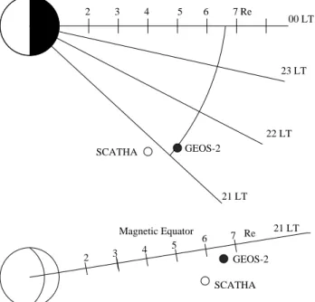
21 LT 22 LT 23 LT 00 LT 2 3 4 5 6 7 GEOS-2 SCATHA Re GEOS-2 SCATHA 2 5 6 4 Magnetic Equator Re 21 LT 3 7
Fig. 1. Schematic illustration of GEOS-2 and SCATHA positions
in the equatorial and meridian planes on 22 May 1979 at 18:40 UT.
These FABCs are indirectly observed by the appearance of azimuthal magnetic field components during substorms (Coleman and McPherron, 1976; McPherron and Barfield, 1980; Kokobun and McPherron, 1981). For symmetry rea-sons, the FABCs should vanish at the magnetic equator, and hence are most clearly observed some distance away from the magnetic equatorial surface (MES).
The region of disrupted current subsequently expands both azimuthally (Nagai, 1991) and radially (Jacquey et al., 1991, 1993), and ultimately, for a fully developed substorm, the entire magnetic field approaches a dipolar structure.
Substorm developments in the magnetosphere may alter-natively be visualized as an expansion of a bounded dipolar-ized region (DPR), with a boundary (or front) separating the tailward and dipolar-like magnetic field structures, respec-tively. The signature of a transition from tailward to dipolar structures can be identified from the meridian magnetic field components.
A statistical study of 194 substorms recorded at geosyn-chronous orbit by the GOES-5 and GOES-6 satellites by Na-gai (1991) indicated, on average, that substorm onsets were located in a narrow sector centered around 23:30 MLT, with subsequent expansions both west- and eastwards. The extent of the disruption region was estimated by Ohtani et al. (1991) to be of the order of, or less than, one Earth radius RE. In
a later work, Ohtani et al. (1998) found by using data from AMPTE/CCE and SCATHA, which were closely spaced in the midnight sector, that the disruption region could be of the order of the proton gyroradius.
The expansion and subsequent dipolarization of the mag-netic field is associated with particle injections which are considered as independent signatures of substorm onset. The
recorded expansion of particle injection fronts exhibits more detailed structure than the corresponding magnetic dipolar-ization, with a time separation of electron and ion injec-tions, depending on the local time. A two-satellite study of 43 substorm events by Thomsen et al. (2001) confirmed the azimuthal expansion of the injection region both west- and eastwards at geostationary distances.
Ohtani et al. (1992) modelled the azimuthal disrupted cur-rent vs. magnetic field and presented a method for analysing radial substorm expansions in the absence of FABCs. Using magnetic field data from the closely positioned s/c ISEE 1 and ISEE 2, a statistical study indicated onset positions for all but one event earthward of the s/c locations at 12–22 RE.
Even if the breakup location was known, one would in gen-eral need sevgen-eral satellites to estimate characteristic sion properties because the DPR may have different expan-sion velocities in different directions as schematically illus-trated by Ohtani et al. (1991).
One of the major problems in understanding substorm onset and development is the substorm trigger mechanism. Based on experimental evidence recorded at geostationary distances, Roux et al. (1991) interpreted the substorm devel-opment in terms of ballooning modes. A number of papers have addressed the ballooning instability in the near-Earth magnetosphere <10 RE(e.g. Miura et al., 1989; Ohtani et al.,
1989a,b; Ohtani and Tamao, 1993; Lee and Wolf, 1992; Lee, 1998; Hurricane et al., 1997; Bhattacharjee et al., 1998a,b; Cheng and Lui, 1998; Horton et al., 1999; Hurricane et al., 1999; Horton et al., 2001).
During several time intervals in 1979–1980 the satellites GEOS-2 and SCATHA were situated relatively close on the nightside of the Earth at geosynchronous distances. Several substorm events have been identified during these periods. In this paper we investigate a substorm which occurred on 22 May 1979, and was recorded on the two closely spaced
s/c. The two s/c were separated by ∼0.65 RE in longitude,
and by ∼0.9 RE in latitude, with GEOS-2 close to the
mag-netic equator and SCATHA close to the current sheet bound-ary. With this constellation we observe both the longitudinal rate of expansion and the latitudinal structure of the FABCs during the substorm.
In Sect. 2 we present the substorm event, and in Sect. 3 we present the data set which is used in Sect. 4 to discuss the re-lations between the FABCs and the time development of the magnetic field components. The possible link between the substorm and a ballooning instability is discussed in Sect. 5. Finally, Sect. 6 summarizes the discussion.
2 Substorm event: 22 May 1979
The data available from GEOS-2 and SCATHA only tially cover the same quantities, frequency ranges, and
par-ticle energy intervals. Among the accessible parameters,
we have used the three components of the magnetic field with a time resolution of 5.5 s for both s/c. On GEOS-2, the two equatorial components (normal to the satellite spin
Table 1. Location of Sodankyl¨a, and footprints of GEOS-2 and
SCATHA, respectively.
SOD SCA GEO 18:30 UT E 26◦380 31◦510 37◦360
N 67◦220 66◦380 69◦000 19:00 UT E 26◦380 33◦090 37◦360 N 67◦220 66◦540 69◦000
axis) of the electric field with the same time resolution of
5.5 s is available. On GEOS-2 we have high frequency
0.1 Hz≤f ≤12 Hz oscillations of the magnetic field com-ponents, while on SCATHA we have recordings of the scalar electric and magnetic fields in different frequency bands in the range 0.1 Hz≤f ≤ 200 Hz. Differential high energy par-ticle fluxes of electrons and ions are available on both s/c with a time resolution of 1 min. On GEOS-2 we use the equatorial plane components of the integrated high energy ion flux intensities with a time resolution of 5.5 s. In ad-dition, we have ground magnetogram recordings of the two horizontal magnetic field components from Sodankyl¨a.
During the selected substorm event on 22 May 1979 at
∼18:40 UT, SCATHA and GEOS-2 were closely situated
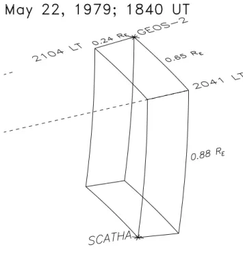
on the evening side of the Earth, as illustrated in Fig. 1 and Fig. 2. Figure 1 shows schematically the location of the two s/c in the equatorial plane and in the meridian (21:00 LT) plane, while Fig. 2 shows a more detailed per-spective of the relative position of the two s/c. At 18:40 UT (21:04 LT), GEOS-2 was in a geostationary orbit at 6.6 RE,
while SCATHA was in a position 6◦to the west of GEOS-2 at
20:41 LT. Further, SCATHA was 0.24 REradially earthward
from GEOS-2, and 7.5◦ below the GEOS-2 orbital plane.
The distance between the two s/c was 1.1 RE.
The estimated footprints for SCATHA and GEOS-2 and the location of the Sodankyl¨a station are summarized in Ta-ble 1. The Sodankyl¨a station was located during the substorm to the west of the footprints of the two s/c. The onset of the dipolarization event occurred around 18:40 UT. The selected time period of 30 min begins at 18:30 UT and covers a 10 min period before the dipolarization onset and the main part of the dipolarization process as observed on the two s/c.
3 Presentation of data
Below, we present diagrams which show the time develop-ment of a number of quantities in the selected time inter-val. The coordinate system used for the data presentation is a satellite centered V DH system, with V radially outward,
Din the azimuthal east direction, and H parallel to the spin axis of the Earth. The general trend is a clear separation into a quiet pre-substorm period ending around 18:40 UT, fol-lowed by a period characterized by a transition to a dipolar
Fig. 2. Relative positions of GEOS-2 and SCATHA on
22 May 1979 at 18:40 UT.
magnetic field structure accompanied by large amplitude os-cillations.
3.1 Magnetic Fields
On both s/c, the recorded magnetic fields cover a wide fre-quency range from 0 to several Hz. The oscillations which are seen on the magnetic (and electric) field components are, to a large extent, associated with the dipolarization process. The low frequency plots exhibit the ambient magnetic field variations with superimposed low frequency oscillations.
3.1.1 GEOS-2 magnetic field
In Fig. 3 the magnetic field components recorded on GEOS-2 illustrate the combined result of a relatively slow average trend, associated with the reconfiguration of the overall mag-netic field, and large amplitude irregular oscillations (Holter et al., 1995). Each magnetic component exhibits a number of minima and maxima whose identification is somewhat uncer-tain due to the superimposed oscillations. After ∼18:40 UT we observe on Fig. 3 large amplitude irregular oscillations on all components, and note the following characteristics:
The BV-component decreases slowly from an initial value
∼7 nT at 18:30 UT to ∼5 nT at ∼18:40:15 UT, when it starts
to increase and attains a first maximum at ∼18:41:15 UT. Subsequent large amplitude low frequency oscillations are superimposed on an average value decaying from 20 to 15 nT.
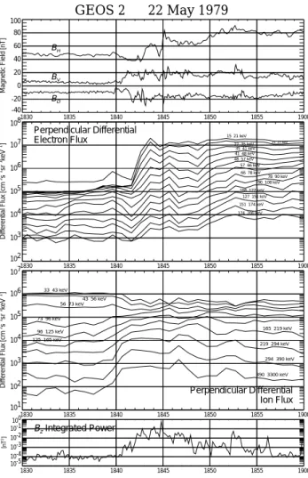
1830 1835 1840 1845 1850 1855 1900 -40 -20 0 20 40 60 80 100 Magnetic Field [nT] BV BH BD 1830 1835 1840 1845 1850 1855 1900 102 103 104 105 106 107 108 Differential Flux [cm − 2s − 1sr − 1keV − 1] 15−21 keV 21−27 keV 27−35 keV 35−41 keV 41−48 keV 48−57 keV 57−66 keV 66−78 keV 78−90 keV 90−108 keV 108−127 keV 127−151 keV 151−174 keV 174−206 keV Perpendicular Differential Electron Flux 1830 1835 1840 1845 1850 1855 1900 101 102 103 104 105 106 107 Differential Flux [cm − 2s − 1sr − 1keV − 1] 33−43 keV 43−56 keV 56−73 keV 73−96 keV 96−125 keV 125−165 keV 165−219 keV 219−294 keV 294−390 keV 390−3300 keV Perpendicular Differential Ion Flux 1830 1835 1840 1845 1850 1855 1900 10-5 10-4 10-3 10-2 10-1 100 [nT 2] Bz Integrated Power GEOS 2 − 22 May 1979
Fig. 3. GEOS-2 measurements as functions of time. From top to
bottom: 1. Three magnetic field components; 2. Differential high energy electron flux intensity; 3. Differential high energy ion flux intensity; 4. Integrated power of magnetic field oscillations in fre-quency range 0.5–11 Hz.
The BD-component is negative (westward) and remains
almost constant around ∼10 nT until ∼18:40 UT. Following a temporary drop in magnitude, an increase accompanied by large amplitude oscillations starts at 18:41:00 UT, and a max-imum level of ∼−20 nT is attained at ∼18:41:45 UT. Except
for some low frequency oscillations, BD remains, on
aver-age, almost constant at ∼−15 nT after ∼18:45 UT. A small decrease after ∼18:57 UT brings the BD-value close to its
initial value ∼−10 nT.
The BH-component remains initially almost constant with
a value ∼48 nT. At ∼18:39:45 UT it starts to decrease to-wards a minimum value ∼40 nT around ∼18:41:30 UT. At
∼18:42:30, BHstarts to increase rapidly in an irregular
fash-ion, and attains an approximate maximum ∼85 nT around
∼18:52:40 UT. 1830 1835 1840 1845 1850 1855 1900 -50 0 50 100 Magnetic Field [nT] BV BH BD 1830 1835 1840 1845 1850 1855 1900 103 104 105 106 107 108 Differential Flux [cm − 2s − 1sr − 1keV − 1] 19.4 keV 57 keV 98 keV 140 keV Perpendicular Differential Electron Flux 1830 1835 1840 1845 1850 1855 1900 103 104 105 106 Differential Flux [cm − 2s − 1sr − 1keV − 1] 15.6 keV 36 keV 71 keV 133 keV Perpendicular Differential Proton Flux 1830 1835 1840 1845 1850 1855 1900 UT 0.0 1.0 2.0 3.0 [TM V]
B-Field ELF Wave
SCATHA − 22 May 1979
Fig. 4. SCATHA measurements as functions of time. From top to
bottom: 1. Three magnetic field components, 2. Differential high energy electron flux intensity. 3. Differential high energy ion flux intensity. 4. Integrated power of magnetic field oscillations in fre-quency range 1.0–2.0 Hz.
3.1.2 SCATHA magnetic field
In Fig. 4 we have plotted the magnetic field components recorded on SCATHA. As on GEOS-2, we observe after
∼18:40 UT irregular oscillations on all components,
how-ever, with relative amplitudes smaller than on GEOS-2. From Fig. 4 we note the following characteristics of the three com-ponents:
The BV-component starts at a value ∼85 nT and then
de-creases slowly to a value of ∼75 nT at ∼18:41:20 UT. An increase to a maximum ∼85 nT at ∼18:43:00 UT is then fol-lowed by a slowly decreasing average value around ∼77 nT.
At ∼18:54:20 UT the BV-value drops further and attains a
value ∼55 nT at ∼18:57:30 UT.
The BD-component on SCATHA starts at 18:30 UT with
a value ∼−8 nT close to the value measured on GEOS-2. However, the magnitude decreases to an average around zero with superimposed low frequency oscillations. Around
SODANKYLA − 22 May 1979 1830 1835 1840 1845 1850 1855 1900 UT -3 -2 -1 0 1 2 3 H -Component [nT] 1830 1835 1840 1845 1850 1855 1900 UT -3 -2 -1 0 1 2 3 D -Component [nT]
Fig. 5. Ground observations of the magnetic H - and D-components
recorded at Sodankyl¨a.
followed at ∼18:41:40 UT by a relatively sharp increase. A maximum negative value of ∼−53 nT is attained at
∼18:43:10 UT. Following a subsequent decrease in its
mag-nitude, BDattains ∼−10 nT at 18:46:15 UT and a minimum
magnitude close to zero at ∼18:47:30 UT. The magnitude of BD then increases and remains fairly constant with slow
variations around ∼−10 nT for t >18 : 50 UT.
The BH-component remains initially almost constant at
a value ∼50 nT until ∼18:40:25 UT, when it starts to
de-crease, reaching a minimum ∼ 35 nT at ≈18:43:00 UT. BH
then increases and attains a maximum close to ∼100 nT at
∼18:57:10 UT.
3.1.3 Sodankyl¨a magnetic field
In Fig. 5 we have plotted the H - and D-components of the ground magnetic field measured at Sodankyl¨a, which is
lo-cated about 11◦to the west of the GEOS-2 magnetic
foot-print. On both components we observe a weak beginning of an intensification at ∼18:37 UT, followed by very strong in-tensifications beginning at ∼18:39 UT, and with a maximum amplitude at ∼18:40 UT. The oscillations persist during the whole time period, however, with amplitudes considerably below the maximum in the later part.
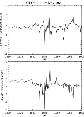
GEOS-2 − 22 May 1979 1830 1835 1840 1845 1850 1855 1900 UT -15 -10 -5 0 5 10 E -Field D -Component [mV/m] 1830 1835 1840 1845 1850 1855 1900 UT -6 -4 -2 0 2 4 6 E -Field V -Component [mV/m]
Fig. 6. Electric field V- and D-components recorded on GEOS-2 as
functions of time.
3.2 Electric field
For GEOS-2 the measured electric field components EV and
EDare presented in Fig. 6. Before ∼18:40 UT, the
measure-ments are unreliable due a bias current that is too small, and the average values appear to be constant offsets.
The EV-component in Fig. 6 exhibits irregular oscillations
around zero. The amplitudes attain values ∼ ±4 mV/m at 18:42:50, 18:45:00, and 18:47:00 UT.
The ED-component in Fig. 6 clearly has an average value
below zero, with irregular superimposed oscillations with maximum amplitudes ∼ ±10 mV/m.
3.3 High energy particle flux intensities
Both on GEOS-2 and SCATHA, measurements of high en-ergy particle fluxes with a time resolution of 1 min are avail-able. The measurements on GEOS-2 include both integrated and differential flux intensities and pitch angle distributions of electron and ion fluxes. The data from SCATHA covers a smaller range of parameters, but the differential high energy particle fluxes are available in energy intervals also covered by the GEOS-2 measurements.
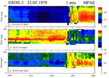
Fig. 7. Pitch angle flux intensities for high energy electrons and
ions recorded on GEOS-2.
3.3.1 GEOS-2 particle flux intensities
In Fig. 3 we show for GEOS-2, the integrated differential fluxes with 1-min resolution for electrons and ions in the pitch angle range 65–115◦. The energy range for electrons
is from 15 to 206 keV, and for ions from 33 keV to 3.3 MeV. The energy intervals represented by the curves are indicated. The 1-min resolution colour diagrams in Fig. 7 show the pitch angle flux intensity distribution for electrons with en-ergies 16.0–213.5 keV, and ions for the two energy ranges 27.5–59.0 keV and 59.0–402.5 keV, respectively.
3.3.2 Electrons
The injection of electrons on GEOS-2 is seen on Fig. 3 as a simultaneous increase of the electron flux intensity on all en-ergy channels at ∼18:41:30 UT. The flux increase is largest for the lowest energy channels. Prior to the injection, at
∼18:39:30 UT, we observe a flux intensity decrease which
is most pronounced for the high energy channels. There is a first maximum, simultaneous an all energy channels, at
∼18:43:30 UT.
The electron pitch angle distribution in Fig. 7 appears close to isotropic prior to the large flux increase associated with the electron injection. At 18:41:30 UT we observe a transition from the near isotropic distribution to a transverse
distribution with a maximum around ∼90◦pitch angles.
3.3.3 Ions
For ions with the highest energies (>219 keV) in Fig. 3, the initial increasing trend appears as dispersive. For the high-est energy channel the flux increase starts at ∼18:37:30 UT, while for the two lower energy channels, it starts one and 2 min later at ∼18:38:30 UT and ∼18:39:30 UT,
respec-tively. For the four intermediate energy channels (73–
219 keV) there is no indication of a dispersive ion injec-tion. For the lowest energies (<73 keV) there is a flux in-tensity decay starting at 18:39:30 UT. The first maxima for
energies >96 keV appear to be attained simultaneously at
∼18:41:30 UT.
For the lowest ion energy interval (27.5–59 keV) in Fig. 7, the pitch angle flux distribution is anisotropic with a
maxi-mum around 90◦. The transverse character of the
distribu-tion is maintained during the whole time period, but with an intensity drop starting at ∼18:40 UT. For the high en-ergy range (59–402.5 keV), the ion flux intensity distribu-tion is anisotropic. Before the injecdistribu-tion, the flux exhibits a minimum for pitch angles around 90◦, indicating a field-aligned velocity distribution. After the injection, beginning at 18:39:30 UT, the anisotropy of the distribution is reversed and attains a maximum around 90◦.
In Fig. 8, top and third panels, the components FV- and FD
represent the integrated ion flux intensity in the radial and az-imuthal directions, respectively. The radial flux, FV, is
alter-natively outwards and inwards. Before onset at ∼18:40 UT the average flux is small and slightly earthward, while later the amplitudes are larger with a negative average value, in-dicating an overall inward ion transport. The average of the
azimuthal flux component, FD, is during the whole period
negative, indicating an overall westward ion transport.
3.3.4 SCATHA particle flux intensities
In Fig. 4 we show for SCATHA the differential fluxes for electrons and ions in the same pitch angle range as for
GEOS-2; i.e. 65◦–115◦. The SCATHA flux data in Fig. 4
covers a smaller energy range than for GEOS-2; four energy channels for electrons from 19.4 keV to 140 keV and four en-ergy channels for ions from 15.6 keV to 133 keV. The respec-tive mean energies for the different channels are indicated on the curves.
3.3.5 Electrons
From Fig. 4, the start of the injection associated with the elec-tron flux intensity increase on SCATHA can be localized to
∼18:42:30 UT for the three highest energy channels. For
the lowest energy channel (19.4 keV), the increase appears to start 1 min earlier at ∼18:41:30 UT. About 2–3 min before the electron injection, at ∼18:40:30 UT and ∼18:39:30 UT, respectively, there is, as on GEOS-2, a flux intensity decrease on all channels. The first electron flux intensity maximum occurs simultaneously on all channels at ∼ 18:44:30 UT.
3.3.6 Ions
For the two highest energy channels (133 and 71 keV) in Fig. 4, the start of the ion flux increase is somewhat uncer-tain, but appears to be at ∼18:37:30 UT and ∼18:38:30 UT, respectively. Although the timing is uncertain, the data do not contradict a dispersive injection of high energy ions. For the two lowest energy channels (15.6 keV and 36.0 keV), the fluxes have a decreasing trend.
1830 1835 1840 1845 1850 1855 1900 -100 -50 0 50 100 150 [10 9 m -2 s -1]
Integrated High Energy Ion Flux (V Component) 1830 1835 1840 1845 1850 1855 1900 -150 -100 -50 0 50 100 (E × B / B 2) V [km s -1] E × B Drift Velocity (V Component) 1830 1835 1840 1845 1850 1855 1900 -80 -60 -40 -20 0 20 40 [10 9 m -2 s -1]
Integrated High Energy Ion Flux (D Component) 1830 1835 1840 1845 1850 1855 1900 UT -100 -50 0 50 100 (E × B / B 2) D [km s -1] E × B Drift Velocity (D Component) GEOS 2 − 22 May 1979
Fig. 8. GEOS-2 measurements as functions of time. From top
to bottom: 1. High energy (>33 keV) radial ion flux intensity; 2. Calculated radial E×B-drift velocity; 3. High energy (>33 keV) azimuthal ion flux intensity; 4. Calculated azimuthal E×B–drift velocity.
3.4 High frequency oscillations
The oscillations associated with the dipolarization extend over a large frequency range from a few mHz to several Hz, and are observed on both s/c. Perraut et al. (2000) interpreted the oscillations with frequencies in the range around ∼1 Hz, the ion cyclotron frequency, as current driven Alfv´en waves, and pointed out that they are consistently observed in con-nection with substorms. The onset of these oscillations is simultaneous with the onset of the substorm and they persist during the selected time interval.
3.4.1 GEOS-2 oscillations
In the lowest panel of Fig. 3 we have plotted the power of the magnetic fluctuations integrated between 0.5 and 11 Hz for the B-components on GEOS-2. The power is approxi-mately constant until 18:40:40 UT when a fast growth starts. These oscillations exhibit several successive maxima; around
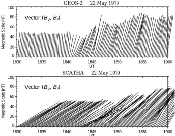
GEOS-2 − 22 May 1979 1830 1835 1840 1845 1850 1855 1900 UT 0 20 40 60 80 100 Magnetic Scale [nT] Vector (BV, BH) SCATHA − 22 May 1979 1830 1835 1840 1845 1850 1855 1900 UT 0 20 40 60 80 100 Magnetic Scale [nT] Vector (BV, BH)
Fig. 9. Vector plots of the meridian plane magnetic field, BH vs.
BV, for GEOS-2 and SCATHA as functions of time.
∼18:43 UT, ∼18:45 UT, ∼18:47 UT, and ∼18:53 UT. The
average amplitude regains its pre–substorm level around
∼18:57 UT.
3.4.2 SCATHA oscillations
The bottom diagram of Fig. 4 illustrates the magnetic power variations recorded on SCATHA in the frequency
inter-val 1.0–2.0 Hz. The onset of these oscillations occur at
∼18:41:30 UT. They persist during the selected time
inter-val, however, with a reduced amplitude after ∼10 min at
∼18:50 UT.
4 Discussion
During the substorm growth-, onset-, and recovery phases, there are large variations in the magnetic and electric fields, electron and ion flux intensities, together with large oscilla-tions over frequency ranges from a few mHz to several Hz. Simultaneous with these magnetospheric processes magnetic Pi2-oscillations are observed on the ground close to the s/c footprint.
4.1 The magnetic field
The variation of the magnetic field during the dipolariza-tion can be illustrated by the vectorial magnetic fields in the meridian V H -plane in Fig. 9 and in the DH -plane in Fig. 10, for GEOS-2 and SCATHA, respectively. To emphasize the overall trend, filtered values have been used (periods >50 s retained). Before the dipolarization, the magnetic field at GEOS-2 is smaller and considerably less tailward directed than at SCATHA. This is consistent with GEOS-2 being be-low, but close to the CS midplane, and SCATHA is presum-ably close to the CS boundary.
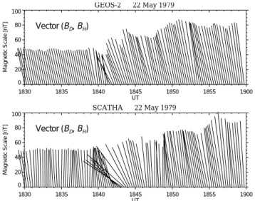
GEOS-2 − 22 May 1979 1830 1835 1840 1845 1850 1855 1900 UT 0 20 40 60 80 100 Magnetic Scale [nT] Vector (BD, BH) SCATHA − 22 May 1979 1830 1835 1840 1845 1850 1855 1900 UT 0 20 40 60 80 100 Magnetic Scale [nT] Vector (BD, BH)
Fig. 10. Vector plots of the magnetic field normal to the meridian
plane, BHvs. BD, for GEOS-2 and SCATHA as functions of time.
4.1.1 Westward expansion
The local commencement of the substorm and the subse-quent magnetic field dipolarization is observed as directional changes of the meridian magnetic fields on GEOS-2 and SCATHA in Fig. 9. The initial indications of a developing substorm on the respective BH-components is first seen on
GEOS-2 at ∼18:39:45 UT, and about 40 s later on SCATHA at ∼18:40:25 UT. The delay indicates an azimuthal westward expansion of the substorm, since an inward radial expansion would first be expected at SCATHA, whose field lines inter-sect the MES farthest from the Earth. The delay observed on SCATHA is also apparent on the other recorded quantities: The ion injection, the initial electron flux decrease, and the electron injection are all delayed by 1 min, which is the reso-lution for the measurements of these quantities. For the quan-tities with higher resolution we estimate the delay between GEOS-2 and SCATHA to be: ∼40 s for the initial B-field stretching, ∼50 s for the onset of high frequency oscillations, and ∼40 s for the dipolarization onset. Further, a westward expansion is not contradicted by the Sodankyl¨a ground ob-servations presented in Fig. 5 which, although the initial am-plitudes are small, may indicate a substorm breakup occur-ring earlier than the first indications on the two s/c. Together with the observed ion flux dispersion, this suggests that the substorm break-up was initiated at a position to the east of the two s/c, and that the subsequent expansion was westward in accordance with the normal tendency established by the find-ings of Nagai (1991), Ohtani and Tamao (1993), and Thom-sen et al. (2001). With an angular s/c separation of 5.75◦at 18:40 UT, we find, with an estimated time delay of ∼45 s, the azimuthal substorm expansion velocity to be ∼7.7◦/min, corresponding to ∼94 km/s at geostationary distances and
∼14 km/s in the ionosphere. Thus, with a breakup in the lo-cal time sector 23:00–24:00 LT, the substorm would, with a
constant expansion velocity, arrive at the GEOS-2/SCATHA position(s) with a delay of about 4–5 min.
4.1.2 Field-Aligned Birkeland Currents (FABC)
At the MES, there is, except for a small azimuthal
compo-nent, only an axial magnetic field component BH. By
def-inition BV is zero. The magnetospheric currents can be
di-vided into currents normal to the magnetic field and Field Aligned Birkeland Currents (FABC). The azimuthal current component at the MES generates magnetic field components
BV and BH in the meridian plane which at the two s/c are
observed as a tailward stretching of the magnetic field dur-ing the substorm growth phase. In situations where FABCs are present, the current-magnetic field relationship is rather complicated. For symmetry reasons, the FABCs vanish at the MES, but off the MES, however, FABCs can generate magnetic fields with all components present. In particular,
1BD changes in the BD-component off the MES, are
inter-preted as a signature of FABCs, e.g. Coleman et al. (1976), McPherron and Barfield (1980), and Kokobun and McPher-ron (1981). Weak FABCs before the substorm onset flow mainly in the meridian plane, but as the substorm devel-ops, and the FABCs become strong, they are tilted in the azimuthal direction along with the magnetic field. The mag-netic field azimuthal tilt, which is seen in Fig. 10 between
∼18:41 UT and ∼18:46 UT, is, as expected from the s/c
po-sitions relative to the MES, most pronounced on SCATHA.
4.1.3 Magnetic field variations
For the discussion of the magnetic field variations, we qual-itatively separate the substorm time sequence into four pe-riods which are closely related to the behaviour of the
az-imuthal BD-component on SCATHA.
4.1.4 BDsmall and positive
According to Fig. 3, the variations of the GEOS-2 magnetic field components are quite small before the substorm on-set. On SCATHA, Fig. 4, however, small but recognizable variations can be identified prior to ∼18:40 UT on all three components. In particular, there is an increase in the BD
-component from a negative value to a value close to zero. For undisturbed conditions at geostationary distances, the
az-imuthal BD-component normally exhibits a small negative
offset (a few nT). Thus, before dipolarization onset, while the s/c is located to the west of the DPR, the increase in BD
indicates the presence of FABCs. The modest magnetic field changes on SCATHA, 1BD>0, 1BV<0, and 1BH>0, are
consistent with weak downward FABCs, both tail- and east-ward of the s/c.
4.1.5 BDnegative and decreasing
Starting at ∼18:39:00 UT the SCATHA azimuthal
BD-component becomes negative followed by a large
can be generated either by an upgoing current tailward, or a
downgoing current earthward of the s/c. The BD-component
thus added to the (meridian) magnetic field results in an azimuthally tilted magnetic field, as seen in Fig. 10, which below the MES conducts azimuthally tilted FABCs. These currents in turn, generate meridian plane magnetic field
components. On SCATHA, beginning at ∼18:40:25 UT,
we observe a decreasing axial BH-component (1BH∼
-20 nT), and, beginning at 18:41:-20 UT, an increasing radial
BV-component (1BV∼15 nT). These changes represent
an additional tailward stretching of the magnetic field, and are consistent with the initial 2-min directional magnetic field change beginning at ∼18:39:45 UT on GEOS-2 and at
∼18:40:25 UT on SCATHA, as seen in Fig. 9. This kind
of tailward magnetic field stretching is a common feature at substorm onset (Kokobun and McPherron, 1981; Nagai, 1982, 1987; Nagai et al., 1987). With the s/c to the west of the approaching substorm, we interpret the observed tailward stretching of the magnetic field (1BV>0; 1BH<0)
on SCATHA as the result of a westward tilted upgoing FABC tailward of the s/c.
4.1.6 BDnegative and increasing
The transition towards a more dipolar-like structure (Fig. 9) begins at ∼18:42:30 UT on GEOS-2 and at ∼18:43:10 UT on SCATHA. The beginning of the dipolar recovery
coin-cides with the minimum values of the axial BH-components
on both s/c as observed on Fig. 3 and Fig. 4 for GEOS-2 and SCATHA, respectively. At SCATHA it closely coincides with both the large maximum magnitude of the negative
az-imuthal component BDat 18:43:10 UT, and the maximum of
the BV-component at 1842:45 UT (Fig. 4). The subsequent
relative variations of the SCATHA magnetic components are:
1BV<0, 1BD>0, and 1BH>0, which are consistent with
an azimuthally receeding upgoing FABC tail- and westward of SCATHA. As seen in Fig. 3, the changes in the magnetic field components are qualitatively similar on GEOS-2, but, except for BH, less pronounced. The weaker response to the
FABCs is consistent with the position of GEOS-2 being close to the MES.
The variations of the magnetic field components suggest that the strong upgoing FABC region moved past SCATHA from east to west on the tailward side. Further, the observed maxima/minima indicate that the central part of the FABC system passed SCATHA at ∼18:43:10 UT and about 45 s earlier for GEOS-2.
4.1.7 BDsmall and positive
After the passage of the strong FABC region, the effect of the FABCs diminish, as clearly observed from the SCATHA
BD-component in Fig. 4, which at ∼18:46 UT attains its
ini-tial value centered around −10 nT. There is, however, a fur-ther decrease in its magnitude to a BD-value around zero, as
observed during the pre–substorm growth period, indicating a possible weak downward FABC tailward of SCATHA for
a 4-min period from ∼18:46 to ∼18:50 UT. The magnetic fields on both s/c approach a dipolar structure, indicating a partially disrupted azimuthal current in the vicinity of the s/c. On SCATHA the final transition towards dipolarization begins at ∼18:55 UT.
A partially disrupted westward azimuthal current can be regarded as the result of a superimposed equivalent eastward current. Below the MES and earthward of this current, the re-sult would be variations 1BH>0 and 1BV<0, while at the
MES, 1BV∼BV∼0. On GEOS-2, a small but long lasting
positive shift 1BV∼10 nT at 18:41 UT is observed,
indi-cating a northward shift of the MES, and thus bringing the relative position of GEOS-2 somewhat below the MES.
The upward FABCs clearly attain a maximum and then di-minish while the (increasing) equivalent eastward azimuthal current, representing the disrupted part of the original cur-rent, gradually becomes dominant. The main part of the upward FABCs lasts for ∼3–4 min, and with the estimated
azimuthal expansion velocity of ∼7.7◦/min may cover an
azimuthal range of ∼22–31◦. As already pointed out, the
SCATHA BD-component (Fig. 4) indicates weaker
downgo-ing field-aligned current structures both before and after the arrival of the upward FABC structure.
4.2 Particle injections
Before the onset of the local dipolarization, the current which maintains the tailward structure is, on the microscopic scale, carried by azimuthally gradient- and curvature-drifting parti-cles. The electrons drifting towards the s/c from the west, are not accelerated prior to the encounter with the DPR, while the ions drifting towards the s/c from the east have traversed the boundary of the DPR.
When the DPR encounter the s/c, the observed electrons (at all energies) are passing from a region of weak tailward magnetic field to a region with stronger dipolar-like field. The expected dispersionless electron flux intensity increase, or electron injection, is confirmed by the differential flux in-tensities presented in the second panels in Figs. 3 and 4 for GEOS-2 and SCATHA, respectively. The estimated electron injection at ∼18:41:30 UT on GEOS-2 and at ∼18:42:30 UT on SCATHA, represents a delay of ∼1 min, which is compa-rable to the time resolution of the measurements.
About 2 min before the electron injection, the flux intensi-ties decrease by almost an order of magnitude for some en-ergy channels on both s/c.
Although the time resolution does not allow a precise tim-ing, these electron “ejections” apparently coincide with the tailward stretching of the magnetic field observed on both s/c about 2 min prior to the start of the dipolarization.
Compared with the electrons, the situation is quite
dif-ferent for the westward drifting ions. The ion
gradient-and curvature-drifts in the dipolarized magnetic field are in the same direction as the westward expansion of the DPR. The first indication of injected ions at GEOS-2 is at ∼18:37:30 UT for the highest energy channel (Fig. 3), while on SCATHA, at a lower energy, it is at ∼18:38:30 UT
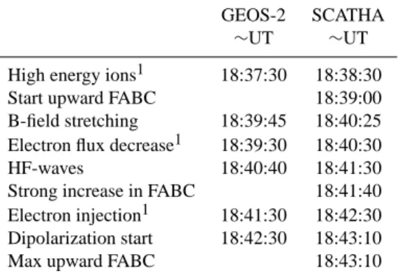
Table 2. Timing of parameter changes at SCATHA and GEOS-2.
GEOS-2 SCATHA
∼UT ∼UT
High energy ions1 18:37:30 18:38:30 Start upward FABC 18:39:00 B-field stretching 18:39:45 18:40:25 Electron flux decrease1 18:39:30 18:40:30 HF-waves 18:40:40 18:41:30 Strong increase in FABC 18:41:40 Electron injection1 18:41:30 18:42:30 Dipolarization start 18:42:30 18:43:10 Max upward FABC 18:43:10
11 min resolution
(Fig. 4). On both s/c there appears to be a dispersion for the highest energy ions which are injected about 4-5 min before the injection of the electrons. It is not possible to identify the time delay between the two s/c from the energy dependent dispersive ion injections.
4.3 Event sequence
Even with a somewhat uncertain timing of the different pro-cesses observed, we may qualitatively and to some extent quantitatively, identify the sequence of events preceeding the substorm dipolarization.
At the position of the two s/c, the first indication of an approaching substorm is the arrival of dispersive high en-ergy ions, with the highest enen-ergy arriving at GEOS-2 at
∼18:37:30 UT and at SCATHA about 1 min later. Then,
on SCATHA at ∼18:39 UT we deduce from the recorded
BD component a change to an upward directed FABC.
At ∼18:39:45 UT on GEOS-2 and about 40 s later, at
∼18:40:25 UT on SCATHA, we observe a tailward
stretch-ing of the meridian magnetic field, whith a simultaneous electron flux decrease on the two s/c. About one min later, we identify on both s/c the onset of high frequency waves; at 18:40:40 UT on GEOS-2 (0.5–11 Hz) and at 18:41:30 UT on SCATHA (1.0–2.0 Hz). Simultaneous with these waves
we note, on basis of the SCATHA BD–component, a rapid
increase in the upward FABC, beginning at ∼18:41:40 UT. At ∼18:41:30 UT and at ∼18:42:30 UT on GEOS-2 and SCATHA, respectively, a strong increase in the electron flux, i.e. electron injection, is observed. The electron injection starts about 1 min prior to the dipolarization onset, which appears on GEOS-2 at ∼18:42:30 UT and on SCATHA at
∼18:43:10 UT. When the dipolarization starts on SCATHA,
we observe a simultaneous minimum of BD, corresponding
to a maximum upward FABC. The event sequence is sum-marized in Table 2.
4.4 Ballooning instability
There has been a number of suggestions related to the mech-anisms which are at the origin of substorm onset and devel-opment. The drift ballooning instability, originally suggested by Roux (1985) and Roux et al. (1991), has clearly been the major candidate to explain the onset and development of sub-storms (e.g. Ohtani et al., 1989a,b; Miura et al., 1989; Ohtani and Tamao, 1993; Lee and Wolf, 1992; Lee, 1998; Hurri-cane et al., 1997; Cheng and Lui, 1998; Bhattacharjee et al., 1998a,b; Horton et al., 1999; Hurricane et al., 1999; Horton et al., 2001).
The ballooning instability mechanism associated with a substorm is qualitatively similar to the Rayleigh–Taylor in-stability. With ion and electron diamagnetic drifts in oppo-site directions and normal to the respective pressure gradients and the magnetic field B, the resulting electron and ion dia-magnetic currents flow along the respective constant pressure surfaces. Prior to substorm onset, during the growth phase, the current sheet is in quasi–equilibrium with the azimuthal diamagnetic current with j being related to the pressure
gra-dient ∇p by j=B×∇p/B2.
With density perturbations of the equilibrium the oppo-site directions of the electron and ion fluxes tend to create space charges. The associated electric fields E, combined with the ambient magnetic field B, result in additional drifts, vE=E×B/B2, which amplify the perturbation. To maintain
quasi–neutrality, any tendency to accumulate space charges is, however, counteracted by neutralizing currents along the magnetic field lines. If these FABCs constitute part of closed current circuits (via the ionoshere), they will tend to neu-tralize the electric fields and thus inhibit the growth of an instability.
Although GEOS-2 and SCATHA are well outside the re-gion of substorm onset, signatures which are associated with ballooning instabilities are observed. These signatures may be of relevance for an understanding of the substorm expan-sion mechanism.
4.4.1 Birkeland currents
The FABCs necessary to maintain quasi-neutrality produce additional magnetic field components. From symmetry rea-sons, these components, as the FABCs, vanish at the MES and increase away from the MES. FABCs in the meridian plane will produce azimuthal magnetic field components, earth- and tailward of the currents, which, in turn modify the direction of the FABCs, which, away from the MES, attain significant azimuthal components.
The difference in the azimuthal magnetic components recorded on the two s/c is evident from Figs. 3 and 4 for
GEOS-2 and SCATHA, respectively. Clearly SCATHA,
which is farthest away from the MES, records the largest val-ues in accordance with what is expected for azimuthal mag-netic field components produced by symmetric FABCs. The
temporary, strong BD-component at SCATHA implies that
direction, is strongly tilted azimuthally across the meridian plane. A FABC will also generate magnetic field components in the V - and H -directions. The recorded changes, 1BV<0
and 1BH>0, are consistent with the s/c being earthward and
initially westward of the FABCs.
4.4.2 E×B dominated radial particle flux
The ballooning instability is associated with ion fluxes in the radial direction composed of both E×B-drifts due to
the ED-component, and diamagnetic drifts caused by the
azimuthal pressure gradient of the perturbation. These ion drifts are 90◦out of phase. Hence, if one of the drifts dom-inates, the measured ion flux oscillations would be either in
phase or 90◦ out of phase with the E×B-drift. In Fig. 8
we present four panels related to the particle fluxes recorded on GEOS-2. The first and the third panel from the top rep-resent the integrated ion flux intensity in the radial and az-imuthal directions for energies >33 keV, respectively, while the second and the fourth panel represent the E×B-drifts in the corresponding directions. Prior to the substorm onset (at
∼18:40 UT) the GEOS-2 electric field cannot be used with
confidence because of a satellite current that is too small. A comparison of the radial ion flux intensity (Fig. 8, top panel) with the radial E×B-drift (Fig. 8, second panel), shows a distinct in phase correlation for the period after 18:40 UT. Thus, the azimuthal electric field, with the associ-ated E×B-drift, dominates the radial particle transport and hence the development of the substorm, as discussed in de-tail by Le Contel (2001) for two other events recorded on GEOS-2. The observed correlation of the E×B-drift and the radial ion flux intensity represents supporting evidence for the presence of ballooning modes during the azimuhal expansion of the substorm.
A similar comparison for the azimuthal ion flux intensity (Fig. 8, third panel) and E×B-drift (Fig. 8, bottom panel), does not reveal similar correlations as for the radial direction. We note, however, the westward azimuthal ion flux, related to the ion curvature and gradient drifts.
5 Summary
A substorm on 22 May 1979 was simultaneously observed on the geosynchronous satellite GEOS-2 and SCATHA when they were separated by less than 30 min in local time, close to 21:00 LT, with SCATHA somewhat earthward of GEOS-2. GEOS-2 was close to the current sheet midplane at the magnetic equatorial surface, while SCATHA was close to the current sheet southward boundary. The first indication of an approaching substorm was the injection of dispersed high energy ions, consistent with high energy ions drifting westward, with a velocity above the substorm expansion ve-locity. The first indication on the magnetic field was recorded about 2 min later as an initial tailward magnetic field stretch-ing, which coincided with a decay of the measured flux inten-sity of ∼ 90◦pitch angle electrons. Apparently, large pitch
angle electrons are first “ejected” before being injected when the magnetic field begins the recovery of a more dipolar-like structure. These substorm onset indications were first recorded on GEOS-2. The estimated delay of 45 to 60 s be-tween the GEOS-2 and SCATHA recordings was consistent with a westward expansion of the substorm boundary, with a velocity of about ∼7.7◦/min. Following the substorm on-set, the most apparent difference in the recordings at the two s/c, was the significantly larger magnitude of the azimuthal magnetic field component recorded on SCATHA. The strong
BD-component at SCATHA lasted about 3 min and was,
to-gether with the variations of the other components BV and
BH, consistent with a strong upward field-aligned Birkeland
current structure below the magnetic equatorial surface. The current structure was moving past the s/c on the tailward side from east to west.
Both before and after the passage of the current structure,
the azimuthal BD-component on SCATHA indicates weak
downward field-aligned currents.
As the large amount of cited papers suggest, the balloon-ing instability is, as suggested by Roux (1985) and Roux et al. (1991), a major candidate for understanding the substorm
onset and development. A simple qualitative (Rayleigh–
Taylor) instability model at the magnetic equator suggests possible ballooning instability signatures. The strong tem-porary azimuthal magnetic field component recorded well below the magnetic equatorial plane at SCATHA, represents a clear signature of strong substorm associated field-aligned currents; the measured radial high energy ion flux is highly correlated with the instability generated E×B-drift during the substorm.
Topical Editor T. Pulkkinen thanks two referees for their help in evaluating this paper.
References
Akasofu, S.-I.: The development of the auroral substorm, Planet. Space Sci., 12, 273, 1964.
Bhattacharjee, A., Ma, Z. W., and Wang, X.: Ballooning instability of a thin current sheet in the high–Lundquist–number magneto-tail, Geophys. Res. Lett. 25, 861–864, 1998a.
Bhattacharjee, A., Ma, Z. W., and Wang, X.: Dynamics of thin current sheets and their disruption by ballooning instabilities: A mechanism for magnetospheric substorms, Phys. of Plasmas, 5, 2001–2009, 1998b.
Cheng, C. Z. and Lui, A. T. Y.: Kinetic ballooning instabil-ity for substorm onset and current disruption observed by AMPTE/CCE, Geophys. Res. Lett., 25, 4091–4094, 1998. Coleman Jr., P. J. and McPherron, R. L.: Fluctuations in the
dis-tant geomagnetic field during substorms: ATS 1, in Particles and Fields in the Magnetosphere, edited by McCormac, B. M., Rei-del, Mass., 171–194, 1976.
Cummings, C. D., Barfield, J. N., and Coleman Jr., P. J.: Magneto-spheric substorms observed at the synchronous orbit, J. Geophys. Res., 73, 6687–6698, 1968.
Fairfield, D. H. and Ness, N. F.: Configuration of the magnetic tail during substorms, J. Geophys. Res., 75, 7032–7047, 1970. Holter, Ø., Altman, C., Roux, A., Perraut, S., Pedersen, A., P´ecseli,
H., Lybekk, B., Trulsen, J., Korth, A., and Kremser, G.: Charac-terization of Low Frequency Oscillations at Substorm Breakup, J. Geophys. Res., 100, 19 109–19 119, 1995.
Horton, W., Wong, H. V., and Van Dam, J. W.: Substorm trigger condition, J. Geophys. Res., 104, 22 745–22 757, 1999. Horton, W., Wong, H. V., Van Dam, J. W., and Crabtree, C.:
Sta-bility properies of high-pressure geotail flux tubes, J. Geophys. Res., 106, 18 803–18 822, 2001.
Hurricane, O. A., Fong, B. H., and Cowley, S. C.: Nonlinear magne-tohydodynamic detonation: Part I, Phys. Plasmas, 4, 3565–3580, 1997.
Hurricane, O. A., Fong, B. H., Cowley, S. C., Coroniti, F. V., Ken-nel, C. F., and Pellat, R.: Substorm detonation, J. Geophys. Res., 104, 10 221–10 231, 1999.
Jacquey, C., Sauvaud, J. A., and Dandouras, J.: Location and propa-gation of the magnetotail current disruption during substorm ex-pansion: Analysis and simulation of an ISSE multi-onset event, J. Geophys. Res. Lett., 18, 389–392, 1991.
Jacquey, C., Sauvaud, J. A., Dandouras, J., and Korth, A.: Tailward propagating cross-tail current disruption and dynamics of near-Earth tail: A multipoint measurement analysis, J. Geophys. Res. Letts., 20, 983–986, 1993.
Kokobun, S. and McPherron, R. L.: Substorm signatures at syn-chronous altitude, J. Geophys. Res., 86, 11 265–11 277, 1981. Lee, D. Y.: Ballooning instability in the tail plasma sheet, Geophys.
Res. Lett., 25, 4095–4098, 1998.
Lee, D. Y. and Wolf, R. A.: Is the Earth’s magnetotail balloon un-stable?, J. Geophys. Res., 97, 19 251–19 257, 1992.
Le Contel, O., Roux, A., Perraut, S., Pellat, R., Holter, Ø., Ped-ersen, A., and Korth, A.: Possible control of plasma transport in the near–Earth plasma sheet via current driven Alfv´en waves (f 'FH +), J. Geophys. Res., 106, 10 817–10 827, 2001. McPherron, R. L.: Substorm related changes in the geomagnetic
tail: The growth phase, Planet. Space Sci., 20, 1521–1539, 1972. McPherron, R. L., Russel, C. T., and Aubry, M. P.: Satellite Stud-ies of Magnetospheric Substorms on 15 August 1968, 9. Phe-nomenological Model of Substorms, J. Geophys. Res., 78, 3131– 3149, 1973.
McPherron, R. L. and Barfield, J. N.: A seasonal change in the effect of field-aligned currents at synchronous orbit, J. Geophys. Res., 85, 6743–6746, 1980.
Miura, A., Ohtani, S., and Tamao, T.: Balloning Instability and Structure of Diamagnetic Hydromagnetic Waves in a Model Magnetosphere, J. Geophys. Res., 94, 15 231–15 242, 1989. Nagai, T.: Observed magnetic substorms signatures at synchronous
altitudes, J. Geophys. Res., 87, 4405–4417, 1982.
Nagai, T.: Field-Aligned Currents Associated with Substorms in the Vicinity of Synchronous Orbit, 2. GOES 2 and GOES 3 Obser-vations, J. Geophys. Res., 92, 2432–2446, 1987.
Nagai, T.: An Empirical Model of Substorm-Related Magnetic Field Variations at Synchronous Orbit, Magnetospheric Sub-storms, in Geophys. Monogr., edited by Kan, J. R. , Potemra, T. A., Kokobun, S., and Iijima, T., 64, 91–95, AGU, Washington D.C., 1991.
Nagai,T., Singer, H. J., Ledley, B. G., and Olsen, R. C.: Field-aligned currents associated with substorms in the vicinity of synchronous orbit, 1. The 5 July 1979 substorm observed by SCATHA, GOES 3, and GOES 2, J. Geophys.Res., 92, 2445– 2431, 1987.
Ohtani, S.: Earthward expansion of tail current disruption: Dual-satellite study, J. Geophys. Res., 103, 6815–6825, 1998. Ohtani, S., Kokobun, S., and Russel, C. T.: Radial expansion of the
tail current disruption during substorms: A new approach to the substorm onset region, J. Geophys. Res., 97, 3129–3136, 1992. Ohtani, S., Miura, A., and Tamao, T.: Coupling between Alfv´en and
slow magnetosonic waves in an inhomogeneous finite-β plasma, I. Coupled equations and and physical mechanism, Planet. Space Sci., 37, 567–577, 1989a.
Ohtani, S., Miura, A., and Tamao, T.: Coupling between Alfv´en and slow magnetosonic waves in an inhomogeneous finite-β plasma, II. Eigenmode analysis of localized ballooning-interchange in-stability, Planet. Space Sci., 37, 579–588, 1989b.
Ohtani, S., Takahashi, K., Higuchi, A., Lui, A. T. Y., Spence, H., and Fennel, J. F.: AMPTE/CCE-SCATHA simultaneous obser-vations of substorm-associated magnetic fluctuations, J. Geo-phys. Res., 103, 4671–4682, 1998.
Ohtani, S., Takahashi, K., Zanetti, L. J., Potemra, T. A., McEn-tire, R. W., and Ijima, T.: Tail current disruption in the geosynchronous region, Magnetospheric Substorms, in Geophys. Monogr., edited by Kan, J. R. , Potemra, T. A., Kokobun, S., and Iijima, T., 64, AGU, Washington D.C., 131–137, 1991.
Ohtani, S. and Tamao, T.: Does the Ballooning Instability Trigger Substorms in the Near-Earth Magnetotail?, J. Geophys. Res., 98, 19 369–19 379, 1993.
Perraut, S., Le Contel, O., Roux, A., Pellat, R., Korth, A., Holter, Ø., and Pedersen, A.: Disruption of parallel current at substorm breakup, J. Geophys. Res. Letts., 27, 4041–4044, 2000. Roux, A., Perraut, S., Robert, P., Morane, A., Pedersen, A.,
Ko-rth, A., Kremser, G., Aparicio, B., Rogers, D., and Pellinen, R.: Plasma Sheet Instability Related to the Westward Traveling Surge, J. Geophys.Res., 96, 17 697–17 714, 1991.
Roux, A.: Generation of field-aligned current structures at sub-storm onsets, in Proceedings ESA Workshop on Future Missions in Solar, Heliospheric, and Space Plasma Physics, Garmisch-Partenkirchen, ESA SP–235, 151, 1985.
Thomsen, M. F., Birn, J., Borovsky, J. E., Morzinski, K., McComas, D. J., and Reeves, G. D.: Two-satellite observations of substorm injections at geosynchronous orbit, J. Geophys. Res., 106, 8405– 8416, 2001.