HAL Id: hal-00295621
https://hal.archives-ouvertes.fr/hal-00295621
Submitted on 21 Jan 2005
HAL is a multi-disciplinary open access
archive for the deposit and dissemination of
sci-entific research documents, whether they are
pub-lished or not. The documents may come from
teaching and research institutions in France or
abroad, or from public or private research centers.
L’archive ouverte pluridisciplinaire HAL, est
destinée au dépôt et à la diffusion de documents
scientifiques de niveau recherche, publiés ou non,
émanant des établissements d’enseignement et de
recherche français ou étrangers, des laboratoires
publics ou privés.
www.atmos-chem-phys.org/acp/5/547/ SRef-ID: 1680-7324/acp/2005-5-547 European Geosciences Union
Chemistry
and Physics
Climatological features of stratospheric streamers in the
FUB-CMAM with increased horizontal resolution
K. Kr ¨uger1,2, U. Langematz1, J. L. Grenfell1, and K. Labitzke1
1Institut f¨ur Meteorologie, Freie Universit¨at Berlin, Germany
2now at: Alfred Wegener Institute for Polar and Marine Research, Potsdam, Germany
Received: 8 September 2004 – Published in Atmos. Chem. Phys. Discuss.: 22 October 2004 Revised: 3 February 2005 – Accepted: 13 February 2005 – Published: 21 February 2005
Abstract. The purpose of this study is to investigate
horizon-tal transport processes in the winter stratosphere using data with a resolution relevant for chemistry and climate mod-eling. For this reason the Freie Universit¨at Berlin Climate Middle Atmosphere Model (FUB-CMAM) with its model top at 83 km altitude, increased horizontal resolution T42 and the semi-Lagrangian transport scheme for advecting passive tracers is used.
A new approach of this paper is the classification of specific transport phenomena within the stratosphere into tropical-subtropical streamers (e.g. Offermann et al., 1999) and polar vortex extrusions hereafter called polar vortex streamers. To investigate the role played by these large-scale structures on the inter-annual and seasonal variability of transport processes in northern mid-latitudes, the global occurrence of such streamers was calculated based on a 10-year model climatology, concentrating on the existence of the Arctic polar vortex. For the identification and counting of streamers, the new method of zonal anomaly was cho-sen. The analysis of the months October-May yielded a maximum occurrence of tropical-subtropical streamers dur-ing Arctic winter and sprdur-ing in the middle and upper strato-sphere. Synoptic maps revealed highest intensities in the sub-tropics over East Asia with a secondary maximum over the Atlantic in the northern hemisphere. Furthermore, tropical-subtropical streamers exhibited a higher occurrence than po-lar vortex streamers, indicating that the subtropical barrier is more permeable than the polar vortex barrier (edge) in the model, which is in good correspondence with observations (e.g. Plumb, 2002; Neu et al., 2003). Interesting for the to-tal ozone decrease in mid-latitudes is the consideration of the lower stratosphere for tropical-subtropical streamers and the stratosphere above ∼20 km altitude for polar vortex stream-ers, where strongest ozone depletion is observed at polar
lat-Correspondence to: K. Kr¨uger
itudes (WMO, 2003). In the lower stratosphere the FUB-CMAM simulated a climatological maximum of 10% occur-rence of tropical-subtropical streamers over East-Asia/West Pacific and the Atlantic during early- and mid-winter.
The results of this paper demonstrate that stratospheric streamers e.g. large-scale, tongue-like structures transport-ing tropical-subtropical and polar vortex air masses into mid-latitudes occur frequently during Arctic winter. They can therefore play a significant role on the strength and variabil-ity of the observed total ozone decrease at mid-latitudes and should not be neglected in future climate change studies.
1 Introduction
In recent years the role of mid-latitude ozone has increas-ingly captured public interest as a substantial decrease of total ozone is not only observed over the winter poles but also at mid-latitudes especially over the northern hemisphere (NH). Maximum ozone loss of up to −6% in winter and up to
−12% in spring occurred over NH mid-latitudes during the early to mid 1990s (Fioletov et al., 2002; WMO, 2003). Be-sides the fundamental chemical processes involved, transport is an important factor in determining the global distribution of atmospheric trace gases, such as ozone.
The overall global transport of trace gases is mainly driven by the mean meridional circulation (MMC) caused by the breaking of planetary and gravity waves in the extratropi-cal stratosphere/ mesosphere, the so-extratropi-called “wave driving” or “extratropical pump” (Haynes et al., 1991; Plumb, 1996). A recent overview of the MMC, also called the Brewer-Dobson circulation (BDC) after its main observational dis-covers Brewer (1949) and Dobson (1956), is given by Plumb (2002).
A quasi isolation of the tropics was first postulated by Plumb (1996) with the concept of the “tropical pipe” model and was proven by the detection of the “tape recorder”
was found in observational and modeling studies, a recent overview of this now called “leaky pipe” model is given by e.g. Plumb (2002). A more comprehensive picture of specific transport processes at the edge and inside the polar vortex was also summarized by that author. More over, horizontal mixing processes through the transport barriers, either by smaller-scale (finger-like) structures (filaments/laminae) or by large-scale (tongue-like) structures (streamers), are thought to play a significant role and are subject of the present paper.
Observational evidence of narrow tongues of tropical air transported into mid-latitudes in the middle stratosphere was shown with low resolution satellite measurements (Leovy et al., 1985; Randel et al., 1993; Manney et al., 1993; Trepte et al., 1993). Rossby wave breaking events at the edge of the tropics and a shift of the polar vortex towards lower lati-tudes seem to be linked with tropical air extrusions into mid-latitudes (Chen et al., 1994; Waugh, 1996). On reaching higher latitudes, these tongues of tropical air are stretched into filaments which are wrapped around the edge of the po-lar night jet (Waugh, 1993). In the present study, the above described phenomena of large-scale, tongue-like features of tropical-subtropical air masses within the stratosphere are called “tropical-subtropical streamers” (Offermann et al., 1999). The term used in this study should not be mistaken with the terminology of “streamers” of a smaller-scale first introduced by Appenzeller and Davies (1992) and Appen-zeller et al. (1996), describing stratospheric intrusions into the troposphere.
Large extrusions of polar vortex air into mid-latitudes in the middle stratosphere were first detected by McIntyre and Palmer (1983; 1984). The authors described the phenom-ena as big “blobs” of potential vorticity (PV), transporting high-latitude air masses equatorward. Due to the breaking of planetary waves at the edge of the polar vortex, these air masses are irreversibly mixed within the surf zone. Waugh et al. (1994b) investigated these large extrusions of polar vortex air with high resolution transport calculations and found that they were characteristic for the middle stratosphere, whose flow is dominated by the increase in amplitude of upward propagating planetary waves. Whereas the same calculations for the lower stratosphere suggested that air ejected from the
dle stratosphere. On the same platform independent mea-surements were carried out with the ATmospheric Trace Molecule Spectroscopy (ATMOS) instrument (Manney et al., 2000), supporting the findings of CRISTA. By compar-ing these measurements with satellite observations and fine scale trajectory calculations, tongue-like phenomena were detected in various trace gases, e.g. CH4, O3, NOx, in the
stratosphere in addition to filament like structures (Manney et al., 2000; Manney et al., 2001).
First evidence of thin, filament-like structures in ozonesonde profiles was given by Brewer and Milford (1960). Such structures are called laminae in vertical space (Dobson, 1973) and filaments in the horizontal plane. These phenomena were observed to have a small vertical extension from 200 m to 2.5 km and to vary between several hundred to a thousand kilometres in horizontal space (Dobson, 1973; Reid and Vaughan, 1991; Reid et al., 1993). Using regu-lar ozonesonde ascents into the stratosphere since the 1960s, these authors found that such phenomena maximize between 12 and 18 km altitude range at high latitudes during the win-ter and spring seasons. They are thought to be mainly excited through differential advection in regions of strong horizon-tal and vertical wind gradients, e.g. in regions of strong jets (Appenzeller and Holton, 1997). The inter-annual, seasonal and long-term variability of laminae has been addressed by many observational studies (e.g. Reid and Vaughan, 1991; Reid et al., 1993; Appenzeller and Holton, 1997; Manney et al., 1998; Reid et al., 1998; Orsolini and Grant, 2000; Wahl, 2002). Strong gradients in the large-scale winds can lead to a layering of the laminae which results in a filament-like structure in the horizontal plane. High resolution transport studies, using contour advection techniques or similar meth-ods, showed the effect of simulating ultra-thin filaments with the use of large-scale winds (e.g. Norton, 1994; Waugh and Plumb, 1994; Chen et al., 1994). Waugh et al. (1994a) and Plumb et al. (1994) demonstrated that these ultra-thin fila-ments of polar vortex extrusions and intrusions were realis-tic features, comparing them with in-situ aircraft measure-ments. These filaments were mainly observed at the edge of the polar vortex in the lower stratosphere, generated by Rossby wave breaking, where they irreversibly mix with the surrounding air masses (Waugh et al., 1994b). A regular oc-currence of filaments of polar vortex extrusions is thought
to play a significant role in the observed total ozone loss in mid-latitudes (Norton and Chipperfield, 1995; Knudsen and Grooß, 2001; Marchand et al., 2003; Millard et al., 2003). These model studies concentrated on investigating smaller-scale, finger-like structures.
Large-scale, tongue-like features or stratospheric stream-ers were successfully simulated with comprehensive models (Mahlmann and Umscheid, 1987; Boville et al., 1991; Rood et al., 1992; Orsolini et al., 1995; Riese et al., 1999; Kouker et al., 1999; Steil et al., 2003). A first climatology of stream-ers was derived with the mechanistic model KArlsruher SIm-ulation of the Middle Atmosphere (KASIMA) using ana-lyzed winds for the winters 1990 to 1998 (Langbein et al., 2001). This “assimilated” streamer climatology was com-pared by Eyring et al. (2003) with simulations from the cou-pled chemistry-climate model ECHAM4.L39(DLR)/CHEM (E39/C). In general a good correspondence between the two was found, when applying the same streamer criterion. How-ever, those authors investigated solely the transport of tropi-cal air into higher latitudes, restricting their intercomparison to the lower stratosphere (21–25 km altitude).
The purpose of this model study is to investigate the pos-sible role of air mass excursions by stratospheric streamers through both transport barriers – the subtropics and the po-lar vortex edge – during Arctic winter. In addition to previ-ous studies, two types of streamers are investigated, tropical-subtropical streamers and polar vortex streamers, using a full climate middle atmosphere model including the whole branch of the BDC.
The paper is organized in the following way: a brief de-scription of the model and the method to identify streamers is given in Sect. 2. The simulation of streamers is presented in a case study in Sect. 3. The inter-annual and seasonal distri-bution of streamers is investigated based on a 10-year model climatology in Sect. 4. The model results are discussed in Sect. 5. Finally, the results are summarized (Sect. 6).
2 Model description and method
2.1 Model
For the streamer study the Freie Universit¨at Berlin Climate Middle Atmosphere Model (FUB-CMAM) with T42 hori-zontal resolution and a semi-Lagrangian transport scheme for advecting tracers is used. The FUB-CMAM is a general circulation model (GCM), run in the standard version with spectral horizontal resolution of T21 (5.6◦×5.6◦) and 34
lay-ers in the vertical with a model top at ∼83 km (0.0068 hPa) altitude and a vertical grid spacing of 3.5 km in the middle atmosphere. A detailed description of the physical param-eterizations is given by Pawson et al. (1998) and the new model configuration is described by Langematz (2000). For the purpose of this study, the horizontal resolution was in-creased to T42 (2.8◦×2.8◦), resulting in a grid mesh distance
of ∼300 km at the equator. Necessary changes in the model code are described in more detail in Kr¨uger (2002). To guar-antee numerical stability in the upper levels the model time step was reduced from 15 to 10 min integration.
2.1.1 Tracer advection
In order to study the transport of trace gases, the FUB-CMAM was coupled with a semi-Lagrangian transport (SLT) scheme with modified exponential splines (B¨ottcher, 1996; Braesicke and Langematz, 1998; Kr¨uger, 2002). The SLT scheme was run with a transport time step of 4 hours and was thus less computer time consuming than Lagrangian schemes. The SLT scheme was used on the same horizon-tal grid of 2.8◦×2.8◦as the model physics and on a vertical grid of 2.4 km equidistant layers throughout the model at-mosphere. To investigate especially horizontal transport pro-cesses in more detail an idealized passive, zonally stratified tracer was advected with zonally homogeneous concentra-tions. The concentration starts with zero at the South Pole and increases up to 180 arbitrary units (au) at the North Pole, with no changes in the vertical. This tracer has no sources and sinks in the model. Due to the limited computer time, the tracer was initialized on the first of October of each model year and advected until the end of May, covering the dynam-ical active period in the northern winter stratosphere. 2.1.2 Model integration
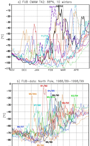
A T42 model run with seasonal variation in solar insola-tion and prescribed climatological sea surface temperatures (SSTs) has been carried out. After two years of initializa-tion, the model was run for 10 years. Time series of the temperature for the grid box closest to the North Pole dur-ing Arctic winters and sprdur-ing are shown in Fig. 1a for the middle stratosphere. A large year-to-year variability in win-ter is simulated solely due to the models’ own inwin-ternal mode of variability. No solar variability, quasi-biennial oscillation (QBO) or volcanic eruptions have been taken into account in the experiment. The simulated strength of variability is com-parable to observed variations during the 1990s, shown here for the FUB observational data (Fig. 1b). For a description of the FUB analysis see e.g. Naujokat et al. (2002). Com-pared to the former T21 model simulations the inter-annual variability has increased. However, the cold pole bias, a fa-miliar feature of GCMs (Pawson et al., 2000), is enhanced compared to observations, apparent in the low temperature of less than −100◦C at 10 hPa during mid and late winter in
se-lected years. The inter-annual variability in the winter strato-sphere is caused by ultra-long planetary waves propagating from the troposphere into the stratosphere where they tend to break and decelerate the stratospheric jet. A detailed anal-ysis, comparing the T42- with former T21-model runs, re-vealed a stronger planetary wave activity but a constant wave mean flow interaction in the T42-simulation (Kr¨uger, 2002).
Fig. 1. Time evolution of the North Pole temperature (◦C) from November to April at 10 hPa for (a) 10 years of FUB-CMAM at 88◦N, (b) FUB observations for the period 1988/89 to 1998/99.
Figure 2 illustrates the amplitudes of the Fourier analyzed zonal wave number-1 (ZW1) and -2 (ZW2) of geopotential height, calculated from daily data, then averaged for the Oc-tober to May period. The characteristic features are simu-lated in the model with a growing amplitude of both wave numbers with increasing height, maximizing between 50 and 60 km altitude at high latitudes, and a smaller amplitude of ZW2 than of ZW1. According to the high variability present in the T42-simulation the amplitude of ZW1 is rather strong compared to observations (not shown). During the 10-year integration two “wave number-1” major mid-winter warm-ings are simulated with a break-down of the polar vortex and a reversal of the zonal mean zonal wind in 60◦N (not shown) in the Arctic winters 02/03 and 10/11 (Fig. 1a).
Fig. 2. Amplitude of the total wave part of geopotential height wave
number-1 (ZW1) and -2 (ZW2) (gpm) averaged from October to May for 10 model years. Contour intervals are 200 gpm with the 100 gpm isoline added (dashed line).
2.2 Streamer criterion
2.2.1 The zonal anomaly method
To identify the location and the shape of streamers in the model, an objective criterion called the zonal anomaly method was developed. Using daily data, the difference in the concentration at each grid point and the zonal mean of the passive tracer is calculated to derive the zonal anomaly field. Analyzing the zonal anomaly, a threshold value is de-fined to identify and count a streamer event. According to the increasing tracer concentration from the South to the North Pole, a positive zonal deviation in the NH indicates high lat-itude air advected into lower latlat-itudes, and a negative devia-tion marks low-latitude air advected into higher latitudes. In the SH the deviation changes sign for both transport cases. Different threshold values were tested for both transport phe-nomena independently, varying from ±15 au to ±25 au. Fi-nally, anomalies of +20 au and more were chosen to identify polar vortex streamers and of −20 au and less to identify tropical-subtropical streamers in the NH. The occurrence of streamers per day at 12:00 UTC and per grid point is counted using this new algorithm. The purpose of this study is to count the total amount of time and location when streamers are present, not the total number of streamer developments. Therefore, the distributions are normalized, resulting in rel-ative frequency of streamers (1.0 ˆ=100%, 0.0 ˆ=0% per time occurrence). The climatology will concentrate on the period October to May and on stratospheric levels. An altitude range from 15–40 km is chosen, sub-divided into 5 equal layers, each containing 2 vertical transport levels, from 16–20 km, 21–25 km, 26–30 km, 31–35 km and 36–40 km altitude.
3 Case study
In this case study the ability of the FUB-CMAM to simulate stratospheric streamers is presented. The objective criterion to identify and count streamers will be demonstrated in de-tail.
3.1 Synoptic situation
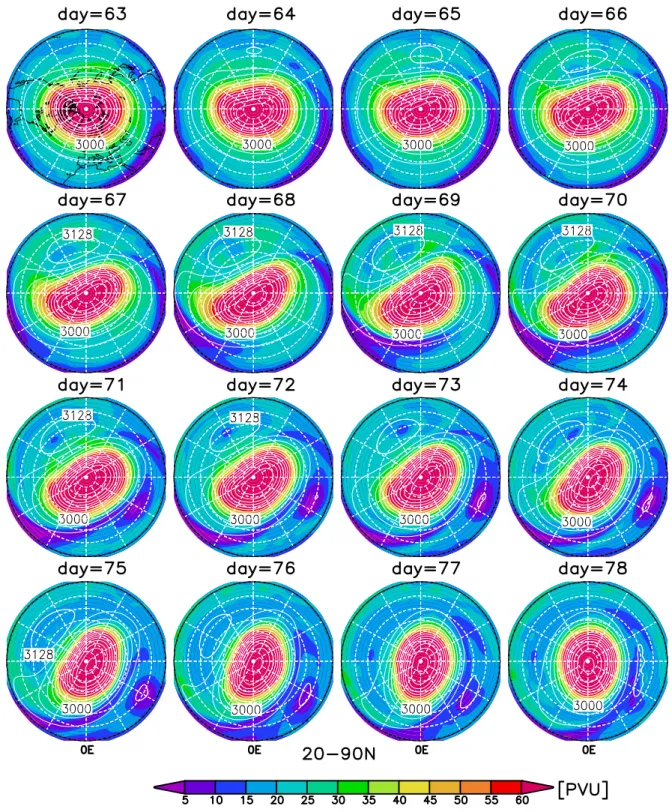
For this case study, a typical cold and undisturbed winter (year 11/12) was chosen (Fig. 1a). Figure 3 shows the syn-optic situation for the early winter period, using geopotential height (at 10 hPa) and PV (at 850 K) fields for the middle stratosphere. On day 63 (3rd December), the centre of the cold vortex is directly situated over the North Pole. One day later an Al¨eutian high begins to form. In the follow-ing days the anticyclone strengthens, pushfollow-ing the vortex cen-tre towards lower latitudes and leading to an elongated po-lar vortex with a zonal wave number-2 pattern. Around day 71, a second anticyclone develops over Eurasia, indicating a strengthening of wave number-2. This dynamical situa-tion can be categorized as a typical “cold wave 2” behaviour (Labitzke, 1977) with an eastward travelling wavenumber-2 characteristic (Kr¨uger et al., 2005), and does usually not cul-minate in a break-down of the polar vortex, i.e. a major mid-winter warming.
Concerning transport processes in the stratosphere, PV on an isentropic level can be regarded to be a quasi-conserved quantity up to 5 days, behaving as a passive tracer. The PV field shows the development of tongues of tropical air over the Atlantic from days 67 to 78 and over East Asia from days 63 to 74. Extrusions of polar vortex air can be seen over the USA on days 69–70 and over the Atlantic on days 76–77, which seem to drop out of the polar vortex in the form of blobs, a couple of days later travel to the tropical belt as was described by McIntyre and Palmer (1983; 1984).
3.2 Simulation of streamers
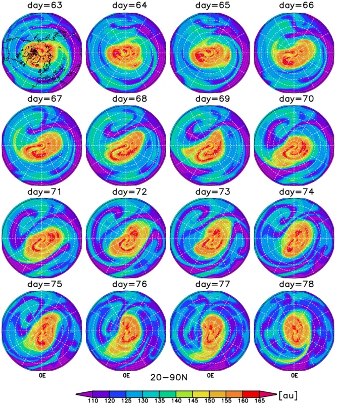
For the same sequence, the passive tracer is shown in Fig. 4. One striking difference to the PV is, that the passive tracer shows a much more differential picture in its evolution. Finer transport structures are conserved in the passive tracer field during the presented period. As can be seen over the West Atlantic, air masses of tropical-subtropical origin are pulled out by the large-scale winds and are advected northeastward over the Atlantic towards Europe (day 67–70). This tongue of tropical air can be identified as an “Atlantic streamer” as defined by Offermann et al. (1999). After day 70 the streamer is advected further northeastward, close towards the edge of the polar vortex, here taken to be the region of max-imum gradient in wind speed. There, the streamer is get-ting longer and thinner by differential advection as was also observed during the first CRISTA experiment. Finally, (af-ter day 72) this “streamer-filament system” begins to
roll-up into a cat eye (McIntyre and Palmer 1983; 1984) over Eurasia, which typically indicates a Rossby wave breaking event associated with irreversible mixing. A simultaneous tropical-subtropical streamer event is visible over East Asia (day 63–74), called an “East Asian streamer” (Offermann et al., 1999), and is also rolling up into a cat eye over the Pa-cific. On days 63, 66, 70 and 78 the evolution of polar vor-tex streamers is visible, which seem to be connected with the development of tropical-subtropical streamers, as was also observed by CRISTA. A more detailed investigation of the processes which produce such transport phenomena was carried out with a correlation analysis of the passive tracer concentration at one grid point with relevant quantities e.g. zonal wind, meridional wind, ZW1, ZW2, PV and geopoten-tial height (not shown). The highest anti-correlations for the “formation” of a tropical-subtropical streamer over the At-lantic on day 69 (see Fig. 4) were obtained by a change to and increase of southerly winds and the equatorward move-ment of the polar vortex. These negative correlations r were higher (r<−0.8) than taking the zonal wind or the zonal wave number-1 and -2 components (r<−0.6). Analyzing the “formation” of a polar vortex streamer is more complex. Cal-culating the correlation for the polar vortex extrusion over the Pacific on day 64 (see Fig. 4) revealed, that the increase of the southerly wind component and the formation of an Al¨eutian high (r<−0.8) were mainly responsible for this event. An-other example over the West Atlantic on day 70 (see Fig. 4) showed that polar vortex streamers can also form in the vicin-ity of the polar vortex edge due to the strong wind gradient, which can lead to a slower advection and pulling out of high tracer gradients into mid-latitude regions. For the further de-velopment of both streamer types a strong wind shear and the differential advection of the high passive tracer gradients are necessary. The breaking or the final stadium of streamers leads to irreversible mixing of tracer contours with the sur-rounding air masses, which is visible for both streamers, e.g. in the cat eye structure over the Pacific on days 67–70 and 75–78 (see Fig. 4). Both type of streamers, namely tropical-subtropical and polar vortex, are found to have a width be-tween 500 to 2000 km and a length of more than 10 000– 20 000 km during the developmental stage. They span a whole latitudinal belt (e.g. the East Asian streamer at day 75). Their duration is between 1–3 weeks and they decay in 1–2 weeks in the model simulations. From this case study, it can be concluded that the main features of the simulated streamers are comparable to those observed during the space shuttle mission in November 1994 (Offermann et al., 1999; Manney et al., 2000; Manney et al., 2001).
3.3 Streamer criterion
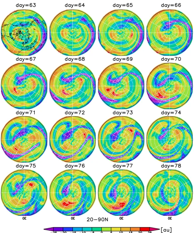
Figure 5 shows the zonal anomaly field with the threshold criteria marked as contour lines for the same time sequence as for Fig. 4. A very good correspondence can be realized be-tween the subjective counting by visible inspection of Fig. 4
Fig. 3. Synoptic development during December days 63 to 78 of year 11. Shown are contour lines (32 gpdam) for geopotential height at
10 hPa and shaded colours for PV at 850 K, from 20–90◦N. 1 PVU (“Potential Vorticity Unit”)=10−5Km2kg−1s−1; 5 PVU intervals.
and the objective method by using the zonal anomaly crite-rion to identify streamers (Fig. 6). For quiet a long period, the polar vortex was shifted off the pole towards lower latitudes, as can be seen in Fig. 3. This dynamical behaviour results in the regular development of tropical air extrusions shown
in Fig. 6. Two pathways are visible for tropical-subtropical streamers, one from the Caribbean Sea over the Atlantic reaching towards Europe/Asia and a second extending from Asia over the Pacific towards Alaska, reaching higher lati-tudes (up to 70◦N) than the Atlantic streamer. Maximum
Fig. 4. Stratospheric streamers simulated in the FUB-CMAM for the same time sequence as in Fig. 3. Shown is the passive tracer [au] at
32 km altitude; 5 au intervals.
intensities of tropical-subtropical streamers, with more than 0.5 relative frequency which corresponds to 50% occurrence in time, are found over the Al¨eutian Islands. This result is not affected qualitatively when changing the threshold num-ber by 25% (±5 au). During this case study, polar vortex streamers only occur for a quarter of the time of the
tropical-subtropical streamers. High intensities with 0.15 relative fre-quency are found over the Atlantic region at mid to high lat-itudes. It is already visible in Fig. 4 that polar vortex stream-ers are weaker phenomena and are therefore detected less readily in this case study.
Fig. 5. Zonal anomaly of stratospheric streamers, as in Fig. 4. Shaded colours represent the anomaly fields and the contours mark the values
of ±20, 25, 30, 35 thresholds.
Different criteria have been tested: the zonal anomaly (this study), the meridional gradient (Eyring et al., 2003) and the vertical gradient methods (e.g. Orsolini and Grant, 2000 and Langbein et al., 2001). For the design of this tracer exper-iment, use of the zonal anomaly method provided the most
convincing results in detecting the horizontal shape of the streamers realistically without any shift in the meridional plane and location as was detected in the meridional gradient method by Eyring et al. (2003). The vertical gradient method (e.g. Orsolini and Grant, 2000 and Langbein et al., 2001) was
Fig. 6. Synoptic maps of relative frequency distributions of (a)
tropical-subtropical streamers and (b) polar vortex streamers for the time sequence shown in Fig. 4.
not appropriate for our model experiments due to the limited vertical resolution. For a more detailed discussion of possi-ble method deficiencies see Sect. 5.
4 Streamer climatology
In this section the zonal anomaly criterion will be used to investigate the occurrence of stratospheric streamers during 10 model years. The main emphasize will be placed on the inter-annual and seasonal variability of such phenomena in the northern winter stratosphere.
4.1 Inter-annual and seasonal variability
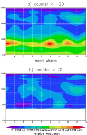
Figure 7 shows the inter-annual variability for (a) tropical-subtropical (counter <−20) and (b) polar vortex streamers (counter >20) in the NH for 10 years. The frequencies are averaged for the October to May period and over the 15– 40 km altitude range. In every winter, a maximum occurs in the subtropics at 25◦N with intensities varying from 3.5% to 6.0% per winter mean, which coincides with the forma-tion region of tropical-subtropical streamers and is proba-bly associated with the reversible distortion of tracer contour lines. In some of the winters the maximum in the subtrop-ics can be tracked towards higher latitudes around 70–75◦N
(e.g. model years 4, 6, 8, 10 and 11), which are tropical-subtropical streamers advected towards higher latitudes and irreversibly mix to a large part within this region. The abso-lute maximum of these signals is reached in year 11 (corre-sponding to winter 11/12) at 70◦N, which shows an anoma-lously high occurrence of tropical air masses at polar lati-tudes (see Sect. 3). In the same winter, an absolute maximum
Fig. 7. Inter-annual variability of relative frequencies of
tropical-subtropical streamers and (b) polar vortex streamers averaged over the October to May period and over 15–40 km altitude, zonal means from 0–90◦N.
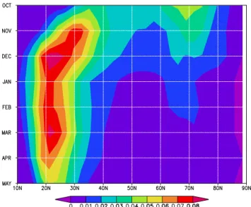
was also found for polar vortex streamer occurrences 10◦ southward (Fig. 7b). In general polar vortex streamers oc-cur less frequently; maximum intensities from 1.5% to 2.0% are reached at 60◦N during year 6 and 11. In model year 9, an extra-tropical air intrusion into the subtropics has taken place, indicating the existence of a leaky subtropical bar-rier in the FUB-CMAM. The seasonal evolution of tropical-subtropical streamers during northern winter is shown with zonal averages over the 15–40 km altitude range for each month in Fig. 8. In the subtropics, the region of streamer development, high frequencies are found from November to April maximizing in December and March. The advection of tropical-subtropical streamers towards higher latitudes seems to be preferred from October to February. Beginning in March, a minimum of streamer frequency is found at mid and high latitudes, indicating more quiescent dynamics due to the existence of easterly winds at polar latitudes. The fre-quency of polar vortex streamers (not shown) reveals a
max-Fig. 8. Seasonal variability (October to May) of relative
frequen-cies of tropical-subtropical streamers averaged over the 15–40 km altitude, zonal means from 10–90◦N.
imum at 60◦N and at 85◦N only from October to February,
whereby a higher occurrence of polar vortex streamers would be expected in spring due to the final break-down of the po-lar vortex, which occurs in the climatological model mean not before June. This discrepancy might be also influenced by a less readily detection of polar vortex streamers due to the weakening gradient of the passive tracer field at higher latitudes to the end of the simulation period caused by nu-merical diffusion of the SLT scheme (see section 5). 4.2 Vertical extension
For the vertical extension of streamers in the stratosphere, winter averages of zonal and area mean frequencies of tropical-subtropical streamers are shown in Fig. 9. The model climatology reveals maximum frequencies of 3% to 9% in the middle and upper stratosphere between 26 to 40 km altitude in the subtropics (Fig. 9a). A clear occurrence of streamers at higher altitudes in the stratosphere is demon-strated by this model study, indicating the role played by the ultra-long planetary waves on the development of strato-spheric streamers, as ZW1 and ZW2 amplitudes grow with increasing altitude (Fig. 2). The area means approach enables us to follow the formation and existence stages of tropical-subtropical streamers (Fig. 9b–e). There are two main re-gions where streamers are excited in the model, mainly over Asia and a secondary region over the West Atlantic. This is visible in the strongest maximum over the 0–90◦E sec-tor, the excitation region of East Asian streamers, and in a smaller maximum over the 0–90◦W sector illustrating a sec-ondary excitation region of Atlantic streamers. After their excitation, tropical-subtropical streamers move progressive with the main flow and poleward. This can be seen by
fol-Fig. 9. Vertical distribution of relative frequencies for
tropical-subtropical streamer averaged over the October to May period for
(a) zonal mean, (b) 0–90◦E, (c) 90–180◦E, (d) 90–180◦W and (e) 0–90◦W.
lowing the first maximum into the 90–180◦E and 90–180◦W sectors and the secondary maximum into the 0–90◦E sector, which then overlaps with the excitation region of the East Asian streamers.
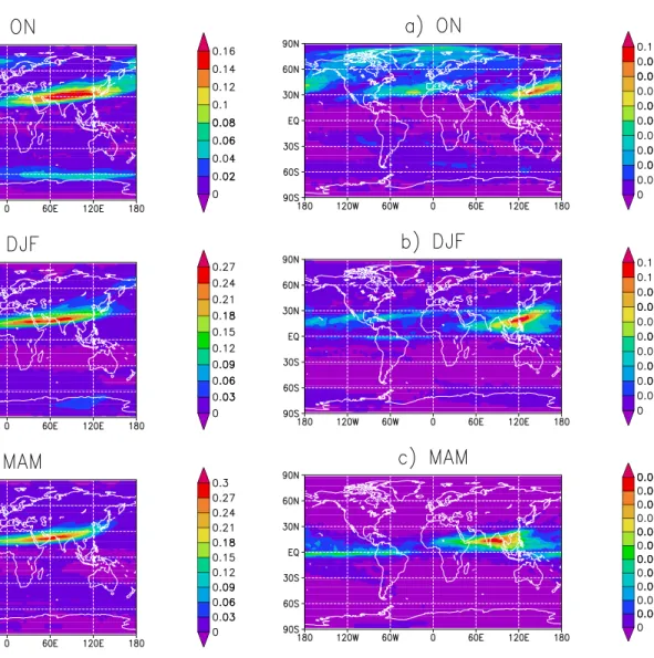
4.3 Synoptic maps
Figure 10 shows the synoptic maps for tropical- subtropical streamers averaged over the October-November (ON), De-cember to February (DJF) and March to May (MAM) periods during the 10 model-years. Maximum frequencies from 0.27 to 0.30 occur for tropical-subtropical streamers during win-ter and spring in the middle stratosphere (31–35 km mean). The band of high intensity extends from the Atlantic towards the Western Pacific for all three periods, containing also the secondary excitation region of the Atlantic streamers, as was visible in Fig. 4. During ON a large region of high intensities is analysed at polar latitudes, reaching from the Al¨eutian Is-lands towards Greenland. This maximum might be artificial as no high has been established in that season in the model. This behaviour may be associated with the time of the year (1st October) or/and the method of initializing the passive tracer (zonally homogeneous), as it takes several days before
Fig. 10. Streamer climatology: synoptic maps of relative frequency
distributions for tropical-subtropical streamer, averaged over 31– 35 km altitude for (a) ON, (b) DJF and (c) MAM period; note the varying contour intervals.
the contours of the passive tracer has adapted to the dynami-cal field.
Interesting for ozone loss at mid-latitudes is the consid-eration of the lower stratosphere, showing a direct influence of natural low-ozone air mass transport into mid-latitudes. Figure 11 displays tropical-subtropical streamer frequencies for the lower stratosphere averaged over 21–25 km altitude. In contrast to the middle stratosphere, maximum intensities occur during early- and mid-winter with only a third less ap-pearance (11% during 10 years) compared with the middle stratosphere. In the lower stratosphere, excitation regions lie over the central Atlantic and over East Asia, tilting westward with increasing height as is visible when comparing Fig. 11 with Fig. 10, indicating the role of planetary waves in these processes. It is apparent that the Atlantic streamer becomes more important towards lower altitudes (21–25 km) whereas
Fig. 11. As in Fig. 10 but for 21–25 km altitude.
the East Asian streamer is most pronounced in the middle stratosphere (31–35 km) during October/November, which is in good correspondence with CRISTA observations (Riese et al., 1999).
4.4 Comparison with observed tropical-subtropical streamer climatologies
The simulated strength of variability of e.g. the North Pole temperature in the stratosphere during Arctic winter is com-parable to the observed inter-annual variability during the 1990s (see Fig. 1). Therefore, the streamer climatology of the T42-model is compared to assimilated streamers from the 1990s, derived with the mechanistic model KASIMA (Lang-bein et al., 2001). Only tropical-subtropical streamers can be compared as no polar vortex streamers have been taken into account by those authors. In the present study, the maxi-mum of tropical-subtropical streamer activity lies in the NH,
ing towards mid-latitudes during winter and spring.
It should be noted however that the main characteristics of the streamer climatology strongly depend on the cho-sen method and the respective streamer criterion. Eyring et al. (2003) analysed the same KASIMA data used by Lang-bein et al. (2001) with the meridional gradient method. Their results differ from Langbein et al. (2001) and other observa-tional estimates (Offermann et al., 1999; Manney et al., 2000; Manney et al., 2001), as maximum streamer intensities were analysed further poleward over Central Europe and the At-lantic in mid-latitudes with a weak secondary maximum in the subtropics over East Asia during winter and spring. The results of the present study are more comparable with results derived from the vertical gradient method used by Langbein et al. (2001) than with those derived from the meridional gra-dient method (Eyring et al., 2003). More research has to be carried out, to determine the reasons for this is beyond the scope of this paper.
5 Discussion
The simulation of streamers in the FUB-CMAM is in very good agreement with most of the streamer observations to date (Offermann et al., 1999; Riese et al, 1999; Manney et al., 2000; Manney et al., 2001). It can be shown with this model study that stratospheric streamers (Offermann et al., 1999) occur preferentially at higher altitudes in the strato-sphere in contrast to filaments/laminae, which were mainly observed in regions between 18–22 km height (e.g. Reid and Vaughan, 1991). Therefore, this streamer climatology cannot be compared with studies which restricted their analyses to filaments or laminae (e.g. Reid and Vaughan, 1991; Reid et al., 1993; Reid et al., 1998; Orsolini and Grant, 2000). Due to limited spatial resolution in the model, filaments/laminae could not be resolved in the experiment. However, it was shown in a case study, that the final stage of a streamer can develop in a filament-like structure, as detected in fine-scale resolution transport studies by e.g. Waugh (1993) and Man-ney et al. (1998). The stretching and thinning of a tropical-subtropical streamer was found close to the edge of the polar vortex, taken here to be the region where maximum wind speeds with the strongest spatial gradient exist. The
theoret-this study. In the process study, the “formation” of tropical-subtropical streamers was found to be higher anti-correlated with the meridional wind components and an equatorward shift of the polar vortex than with an increase of the zonal wind component and the zonal wave numbers-1 and -2.
When comparing this study to other streamer climatolo-gies (Langbein et al., 2001; Eyring et al., 2003), a good correspondence between the general distribution of stream-ers is found only when a similar criterion method was cho-sen. The method used to identify streamers determines to a large extent the results of the climatology. In this study, the streamer climatology based on the method of zonal anomaly, was the best approach to identify streamers in the horizon-tal plane. Nevertheless, method deficiencies due to an arti-ficial counting of streamers can arise in regions with strong horizontal gradients in the passive tracer field: (a) the trop-ical tropopause region due to a too cold and high troptrop-ical tropopause in the model; (b) the subtropics and (c) the polar vortex edge. These artifacts are visible through an enhanced zonal band in the relative frequency field, which did not ef-fect the region of comparison (20–70◦N/S). Another
expla-nation for the deviations could be the use of different passive tracers in the different model studies. Langbein et al. (2001) and Eyring et al. (2003) used chemical N2O fields in contrast
to the idealized, zonally stratified passive tracer without any sources and sinks in this model study.
The higher occurrence of tropical-subtropical streamers compared to polar vortex streamers indicates, that the sub-tropical barrier is more permeable than the polar vortex bar-rier in the T42 FUB-CMAM. This model behaviour is in very good correspondence with observed characteristics of the transport barriers (e.g. Plumb, 2002; Neu et al., 2003). In this model study and in CRISTA observations polar vor-tex streamers seem to be weaker phenomena than tropical-subtropical streamers. The use of a constant threshold num-ber during one winter season could therefore have impacted the detection of stratospheric streamers. Testing the passive tracer fields for the start and the end points of the advection periods reveal a loss of the maximum tracer concentrations of up to 20% at high latitudes in dynamical perturbed winters, which could result in a less readily detection of polar vortex streamers at the end of them. Future investigations of the oc-currence of streamer-like and filament-like structures based
on data with higher vertical and horizontal resolutions would benefit from using a combination of the vertical gradient and zonal anomaly method.
It should be noted that possible model deficiencies could also have an effect on the reliability of the results: the model climatology; the quality of the transport scheme; the use of an idealized zonally stratified tracer and the lower spatial resolution of the FUB-CMAM compared to high resolution transport calculations (e.g. Norton, 1994).
6 Summary
To investigate the influence of large-scale structures on the variability of transport processes in mid-latitudes, a global streamer climatology for 10-years was calculated using the FUB-CMAM with increased horizontal resolution. Unique to this study, the streamer climatology was divided into tropical-subtropical and polar vortex streamers, using a full climate middle atmosphere model including the troposphere, stratosphere and mesosphere.
Stratospheric streamers are regularly simulated with the FUB-CMAM and are in good correspondence with the ob-served features to date. They are characterized as having more than 10–20 km thickness in the vertical, a width be-tween 500 to 2000 km and a length of more than 10 000– 20 000 km during the development stage. They can even span a whole latitudinal belt, as was also analysed for polar vor-tex filaments by e.g. Waugh et al. (1994a) and Manney et al. (2001). Their duration is between 1–3 weeks and they de-cay in 1–2 weeks in the model simulations, which is in good agreement with CRISTA observations. Stratospheric stream-ers have thus to be distinguished from filaments/laminae, de-fined after Reid and Vaughan (1991). However, a streamer can eventually develop into a filament-like structure (e.g. Waugh, 1993; Manney et al., 1998).
An overall result of the streamer climatology is that tropical-subtropical streamers have a higher frequency than polar vortex streamers. This result indicates that the subtrop-ical barrier is more permeable than the polar vortex barrier in the model, which is in good correspondence with obser-vations (e.g. Neu et al., 2003). During the existence of the Arctic polar vortex, the maximum occurrence of tropical-subtropical streamers is up to 30% per 10 years during winter and spring in the middle and upper stratosphere of the NH, where the ultra-long planetary waves are intensified. Synop-tic maps reveal two maxima in the subtropics, one over East Asia and the other over the Atlantic.
Interesting for total ozone concentrations in mid-latitudes are tropical-subtropical transport processes in the lower stratosphere, which are likely to play a significant role in its observed negative trend (e.g. WMO, 2003; Grewe et al., 2004). It is found, that the transport out of the tropics is greater in the middle stratosphere than in the lower strato-sphere, as was also observed by e.g. Chen et al. (1994) and
Waugh (1996). Our investigation of the lower stratosphere revealed the highest occurrence of up to 10% in 10 years of tropical-subtropical streamers from October to February over East Asia/Pacific with a secondary maximum over the Atlantic. These results are in good correspondence with as-similations from the 1990s, if a similar streamer criterion is chosen (Langbein et al., 2001). Observational based stud-ies showed an increase of ozone minima over Europe in the lowermost stratosphere since the late 1980s, indicating an in-crease of subtropical air intrusions into mid-latitudes over Europe (Reid et al., 2000; Bojkov and Balis, 2001), which was confirmed by the study of Koch et al. (2002).
When interpreting these results one has to bear in mind, that the model generaly simulates weak easterly winds in the tropical lower stratosphere. During the easterly phase of the QBO a steeper subtropical tracer isoline slope is observed suggesting a suppressed role of isentropic mixing by eddies particularly in the lower stratosphere (Gray and Russell III, 1999). The same authors also showed a distinct difference between lower and middle stratosphere transport processes in the subtropics with the latter showing an increasing role of isentropic mixing at higher levels which is in good corre-spondence with the main findings of this paper.
Further observational and modeling studies are needed to understand more about the role of streamers in contrast to filaments/laminae in the stratosphere and in particular their role on the observed mid-latitude ozone decrease. Of particular interest would be to investigate the occur-rence of such streamers in transient climate simulations to detect possible trends and influences on the mid-latitude total ozone distribution. An earlier model study with the FUB-CMAM investigating past and present climate changes due to prescribed stratospheric ozone decrease and greenhouse gas increases (Langematz et al., 2003) did not show a statistically significant increase in planetary wave activity, which would have an impact on the occurrence of stratospheric streamers. Until now, a reliable prediction of planetary wave activity and possible future trends for the inter-annual variability during Arctic winter is not feasible, given the large spread in the results of future simulations with coupled chemistry climate models (WMO, 2003).
This study used a new approach, separating stratospheric streamers (broad, large-scale, tongue-like structures) of trace gases or potential vorticity from filaments/laminae (thin, smaller-scale, finger-like structures) first detected in ozonesonde profiles. Specific transport climatologies based on observations have concentrated on the effect of trans-port processes induced by smaller-scale phenomena. In the 10-year climatology, stratospheric streamers are regu-larly simulated with the FUB-CMAM and are in good cor-respondence with the so far observed features. Tropical-subtropical streamers mark the entry of ozone-poor air from the tropics into mid-latitudes in the lower stratosphere. Po-lar vortex streamers mark the entry of chemically processed
Acknowledgements. We thank P. Mieth and P. Braesicke for the support with the model code. For helpful discussions and com-ments we would like to thank I. Langbein, M. M¨uller, T. Shepherd, two anonymous reviewers and H. Wernli. This work was part of the PhD thesis by K. Kr¨uger, funded by the Bundesministerium f¨ur Bildung und Forschung (BMBF) HGF-ENVISAT project (01SF9958). L. Grenfell was supported by the BMBF, grant number 01LG0001, as part of the MESA project. The GCM simulations were performed at the Konrad-Zuse-Zentrum f¨ur Informationstechnik, Berlin.
Edited by: K. Hamilton
References
Appenzeller, C. and Davies, H. C.: Structure of stratospheric intru-sions into the troposphere, Nature, 358, 570–572, 1992. Appenzeller, C. and Holton, J. R.: Tracer lamination in the
strato-sphere: A global climatology, J. Geophys. Res., 102, 13 555– 13 569, 1997.
Appenzeller, C., Davies, H. C., and Norton, W. A.: Fragmentation of stratospheric intrusions, J. Geophys. Res., 101, 1435–1456, 1996.
B¨ottcher, M.: A Semi-Lagrangian Advection Scheme with modified Exponential Splines, Mon. Wea. Rev., 124, 716–729, 1996. Bojkov, R. D. and Balis, D. S.: Characteristics of episodes with
ex-tremely low ozone values in the northern middle latitudes 1957– 2000, Ann. Geophys., 19, 797–807, 2001,
SRef-ID: 1432-0576/ag/2001-19-797.
Boville, B. A., Holton, J. R., and Mote, P. W.: Simulation of the Pinatubo aerosol cloud in general circulation model, Geophys. Res. Lett., 18, 2281–2284, 1991.
Braesicke, P. and Langematz, U.: Coupling of a semi Langrangian transport scheme to the Berlin TSM GCM, Report of MPI for Meteorology, 265, 93–95, 1998.
Brewer, A. W.: Evidence for a world circulation provided by the measurements of helium and water vapor distribution in the stratosphere, Quart. J. R. Met. Soc., 75, 351–363, 1949. Brewer, A. W. and Milford, J. R.: The Oxford-Kew ozonesonde,
Proc. R. Soc., A256, 470–495, 1960.
Calisesi, Y., Wernli, H., and K¨ampfer, N.: Midstratospheric ozone variability over Bern related to planetary wave activity during the winters 1994/95 to 1998/99, J. Geophys. Res., 106, 7903–7916, 2001.
tions estimated from ground-based and satellite measurements: 1964-2000, J. Geophys. Res., 107, 4647, doi:10.1029/JD001350, 2002.
Gray, L. and Russell III, J. M.: Interannual variability of trace gases in the subtropical winter stratosphere, J. Atmos. Sci., 977–993, 1999.
Grewe, V., Shindell, D. T., and Eyring, V.: The impact of horizontal transport on the chemical composition in the tropopause region: Lightning NOx and streamers, Advances in Space Research, 33, 1058-1061, 2004.
Haynes, P., Marks, C., McIntyre, M., Shepherd, T., and Shine, K.: On the ,,Downward Control” of extratropical diabatic circula-tions by eddy-induced mean zonal forces, J. Atmos. Sci., 48, 651–679, 1991.
Holton, J. R., Haynes, P. H., McIntyre, M. E., Douglass, A. R., Rood, R. B., Pfister, L.: Stratosphere-troposphere exchange, Rev. Geophys., 33, 403–439, 1995.
Knudsen, B. M. and Grooß, J.-U.: Northern midlatitude strato-spheric ozone dilution in spring modeled with simulated mixing, J. Geophys. Res., 105, 6885–6890, 2000.
Koch, G., Wernli, H., Staehelin, J., and Peter, T.: A Lagrangian analysis of stratospheric ozone variability and long-term trends above Payerne (Switzerland) during 1970–2001, J. Geophys. Res., 102, 13555–13569, 2002.
Kouker, W., Offermann, D., K¨ull, V., Reddmann, T., Ruhnke, R., and Franzen, A.: Streamers observed by the CRISTA experiment and simulated in the KASIMA model, J. Geophys. Res., 104, 16405–16418, 1999.
Kr¨uger, K.: Untersuchung von Transportprozessen in der Stratosph¨are: Simulationen mit einem globalen Zirkulation-smodell, Dissertation am Fachbereich Geowissenschaften der Freien Universit¨at Berlin, pp. 158, 2002.
Kr¨uger, K., Naujokat, B., and Labitzke, K.: The unusual midwinter warming in the southern hemisphere stratosphere 2002: a com-parison to northern hemisphere phenomena, J. Atmos. Sci., in press, 2005.
Labitzke, K.: Interannual variability of the winter stratosphere in the northern hemisphere. Mon. Weath. Rev., 105, 762–770, 1977. Langbein, I., Kouker, W., Reddmann, T., and Ruhnke, R.: Klima-tologie von Streamern in der unteren Stratosph¨are, Proc. of the DACH conference, 27/399, Wien, 2001.
Langematz, U.: An estimate of the impact of observed ozone losses on stratospheric temperature, Geophys. Res. Lett., 27(14), 2077– 2080, 2000.
Langematz, U., Kunze, M., Kr¨uger, K., Labitzke, K., and Bodeker, G.: Thermal and dynamical changes of the stratosphere since
1979 and their link to ozone and CO2changes, J. Geophys. Res., 108, doi:10.1029/2002JD002977, 4429, 2003.
Leovy, C. B., Sun, C-R., Hitchman, M. H., Remsberg, E. E., Russell III, J. M., Gordley, L. L., Gille, J. C., and Lyjak, L. V.: Transport of ozone in the middle stratosphere: Evidence for planetary wave breaking, J. Atmos. Sci., 42, 230-244, 1985.
Mahlmann, J. D. and Umscheid, L. J.: Comprehensive modeling of the middle atmosphere: the influence of horizontal resolution, Editors G. Visconti and R. Garcia, Transport processes in the middle atmosphere, 251–266, by D. Reidel publishing company, 1987.
Manney, G. L., Michelsen, H. A., Irion, F. W., Toon, G. C., Gun-son, M. R., and Roche, A. E.: Lamination and polar vortex de-velopment in fall from ATMOS long-lived gases observed during November 1994, J. Geophys. Res., 105, 29023–29038, 2000. Manney, G. L., Bird, J. C., Donovan, D. P., Duck, T. J., Whiteway,
J. A., Pal, S. R., and Carswell, A. I.: Modeling ozone laminae in ground-based Arctic wintertime observations using trajectory calculations and satellite data, J. Geophys. Res., 103, 5797–5814, 1998.
Manney, G. L., Froidevaux, L., Waters, J. W., Elson, L. S., Fish-bein, E. F., Zurek, W., Harwood, R. S., and Lahoz, W. A.: The evolution of ozone observed by UARS MLS in the 1992 late win-ter southern polar vortex, Geophys. Res. Lett., 20, 1279–1282, 1993.
Manney, G. L., Michelson, H. A., Bevilacqua, R. M., Gunson, M. R., Irion, F. W., Livesey, N. J., Oberheide, J., Riese, M., Rus-sel III, J. M., Toon, G. C., and Zawodny, J. M.: Comparison of satellite ozone observations in coincident air masses in early November 1994, J. Geophys. Res., 106, 9923–9944, 2001. Marchand, M., Godin, S., Hauchecorne, A., Lev`efre, F., Bekki, S.,
and Chipperfield, M.: Influence of polar ozone loss on North-ern mid-latitude regions estimated by a high resolution chemistry model during winter 1999–2000, J. Geophys. Res., 108, 8326, doi:10.1029/2001JD000906, 2003.
McIntyre, M. E. and Palmer, T. N.: Breaking planetary waves in the stratosphere, Nature, 305, 593–600, 1983.
McIntyre, M. E. and Palmer, T. N.: The ‘surf zone’ in the strato-sphere, J. Atmos. Terr. Physics, 46, 825–849, 1984.
Millard, G. A., Lee, A. M., and Pyle, J. A.: A model study of the connection between polar and mid-latitude ozone loss in the northern hemisphere lower stratosphere, J. Geophys. Res., 108, 8323, doi:10.1029/2001JD000899, 2003.
Mote, P. W., Rosenlof, K. H., McIntyre, M. E., Carr, E. S., Gille, J. C., Holton, J. R., Kinnersly, J. S., Pumphrey, H. C., Russell III, J. M., and Waters, J. W.: An atmospheric tape recorder: The im-print of tropical tropopause temperatures on stratospheric water vapor, J. Geophys. Res., 101, 3989–4006, 1996.
Naujokat, B., Kr¨uger, K., Matthes, K., Hoffmann, J., Kunze, M., and Labitzke, K.: The early major warming in December 2001 – exceptional?, Geophys. Res. Lett, 29(21), 2023, doi: 10.1029/2002GL015316, 2002.
Neu, J. L., Sparling, L. C., and Plumb, R. A.: Variability of the subtropical “edges” in the stratosphere, J. Geophys. Res., 4482, doi:10.1029/2002JD002706, 2003.
Norton, W. A.: Breaking Rossby waves in a model stratosphere diagnosed by a vortex-following coordinate system and a tech-nique for advecting material contours, J. Atmos. Sci., 654–673, 51, 1994.
Norton, W. A. and Chipperfield, M. P.: Quantification of the trans-port of chemically activated air from the northern hemisphere polar vortex, J. Geophys. Res., 100, 25 817–25 840, 1995. Offermann, D., Grossmann, K.-U., Barthol, P., Knieling, P., Riese,
M., and Trant, R.: CRyogenic Infrared Spectrometers and Tele-scopes for the Atmosphere (CRISTA) experiment and middle at-mosphere variability, J. Geophys. Res., 104, 16311–16325, 1999. Orsolini, Y. J. and Grant, W. B.: Seasonal formation of nitrous oxide laminae in the mid and low latitude stratosphere, Geophys. Res. Lett., 27, 1119–1122, 2000.
Orsolini, Y. J., Cariolle, D., and D´equ´e, M.: Ridge formation in the lower stratosphere and its influence on ozone transport: A gen-eral circulation model study during late January 1992, J. Geo-phys. Res., 100, 11 113–11 135, 1995.
Pawson, S., Langematz, U., Radek, G., Schlese, U., and Strauch, P.: The Berlin Troposphere-Stratosphere-Mesosphere GCM: Sensi-tivity to physical parameterizations, Quart. J. R. Met. Soc., 124, 1343–1371, 1998.
Pawson, S., Kodera, K., Hamilton, K., Shepherd, T. G., Beagley, S. R., Boville, B. A., Farrara, J. D., Fairlie, T. D. A., Kitoh, A., Lahoz, W. A., Langematz, U., Manzini, E., Rind, D. H., Scaife, A. A., Shibata, K., Simon, P., Swinbank, R., Takacs, L., Wil-son, R. J., Al-Saadi, A. A., Amodei, M., Chiba, M., Coy, L., de Grandpre, J., Eckman, R. S., Fiorino, M., Grose, W. L., Koide, H., Koshyk, J. N., Li, D., Lerner, J., Mahlman, J. D., McFarlane, N. A., Mechoso, C. R., Molod, A., O’Neill, A., Pierce, R. B., Randel, W. J., Rood, R. B., and Wu, F.: The GCM-Reality In-tercomparison Project for SPARC (GRIPS): Scientific issues and initial results, Bull. Am. Meteorol. Soc., 81, 781–796, 2000. Plumb, R. A.: A “tropical pipe” model of stratospheric transport, J.
Geophys. Res., 3957–3972, 101, 1996.
Plumb, R. A.: Stratospheric Transport, J. Meteor. Soc. Japan, 80, 793–809, 2002.
Plumb, R. A., Waugh, D. W., Atkinson, R. J., Newman, P. A., Lait, L. R., Schoeberl, M. R., Browell, E. V., Simmons, A. J., and Loewenstein, M.: Intrusions into the lower stratospheric Arctic vortex during the winter of 1991/92, J. Geophys. Res., 1089– 1105, 99, 1994.
Randel, W. J., Gille, J. C., Roche, A. E., Kumer, J. B., Mergen-thaler, J. L., Waters, J. W., Fishbein, E. F., and Lahoz, W. A.: Stratospheric transport from the tropics to middle latitudes by planetary wave mixing, Nature, 365, 533–535, 1993.
Reid, J. S. and Vaughan, G.: Lamination in ozone profiles in the lower stratosphere, Quart. J. R. Met. Soc., 117, 825–844, 1991. Reid, J. S., Tuck, A. F., and Kiladis, G.: On the changing abundance
of ozone minima at northern latitudes, J. Geophys. Res., 105, 12 169–12 180, 2000.
Reid, J. S., Vaughan, G., and Kyr¨o, E.: Occurrence of ozone lami-nae near the boundary of the stratospheric polar vortex, J. Geo-phys. Res., 98, 8883–8890, 1993.
Reid, J. S., Rex, M., von der Gathen, P., Floisand, I., Stordal, F., Carver, G. D., Beck, A., Reimer, E., Kr¨uger-Carstensen, R., De Haan, L. L., Braathen, G., Dorokhov, V., Fast, H., Kyr¨o, E., Gil, M., Litynska, Z., Molyneux, M., Murphy, G., O’Connor, F., Ravegnani, F., Varotsos, C., Wenger, J., and Zerefos, C.: A study of ozone laminae using diabatic trajectories, contour advection and photochemical trajectory model simulations, J. Atm. Chem., 30, 187–207, 1998.
dispersal of Mount Pinatubo volcanic aerosol, J. Geophys. Res., 98, 18 563–18 574, 1993.
Wahl, P.: Messung und Charakterisierung laminarer Ozon-strukturen in der polaren Stratosph¨are, Dissertation, an der Mathematisch-Naturwissenschaftlichen Fakult¨at der Universit¨at Potsdam, pp. 142, 2001.
lone, L. M., Webster C. R., and May, R. D.: Transport out of the lower stratospheric Arctic vortex by Rossby wave breaking, J. Geophys. Res., 99, 1071–1088, 1994b.
World Meteorological Organization WMO: Scientific Assessment of Ozone Depletion: 2002, World Meteorological Organiza-tion, Global Ozone Research and Monitoring Project–Report, 47, 2003.