Research on the initial abstraction ? storage ratio and its effect on hydrograph simulation at a watershed in Greece

(1)

HAL Id: hal-00298858

https://hal.archives-ouvertes.fr/hal-00298858

Submitted on 9 Jul 2007

HAL is a multi-disciplinary open access

archive for the deposit and dissemination of sci-entific research documents, whether they are pub-lished or not. The documents may come from teaching and research institutions in France or abroad, or from public or private research centers.

L’archive ouverte pluridisciplinaire HAL, est destinée au dépôt et à la diffusion de documents scientifiques de niveau recherche, publiés ou non, émanant des établissements d’enseignement et de recherche français ou étrangers, des laboratoires publics ou privés.

Research on the initial abstraction ? storage ratio and

its effect on hydrograph simulation at a watershed in

Greece

E. A. Baltas, N. A. Dervos, M. A. Mimikou

To cite this version:

E. A. Baltas, N. A. Dervos, M. A. Mimikou. Research on the initial abstraction ? storage ratio and its effect on hydrograph simulation at a watershed in Greece. Hydrology and Earth System Sciences Discussions, European Geosciences Union, 2007, 4 (4), pp.2169-2204. �hal-00298858�

(2)

HESSD

4, 2169–2204, 2007

Initial

abstraction-storage ratio and hydrograph

simulation E. A. Baltas et al. Title Page Abstract Introduction Conclusions References Tables Figures ◭ ◮ ◭ ◮ Back Close

Full Screen / Esc

Printer-friendly Version

Interactive Discussion

Hydrol. Earth Syst. Sci. Discuss., 4, 2169–2204, 2007 www.hydrol-earth-syst-sci-discuss.net/4/2169/2007/ © Author(s) 2007. This work is licensed

under a Creative Commons License.

Hydrology and Earth System Sciences Discussions

Papers published in Hydrology and Earth System Sciences Discussions are under open-access review for the journal Hydrology and Earth System Sciences

Research on the initial abstraction –

storage ratio and its effect on hydrograph

simulation at a watershed in Greece

E. A. Baltas1, N. A. Dervos2, and M. A. Mimikou3

1

Assistant Professor, Department of Hydraulics, Soil Science and Agricultural Engineering School of Agriculture, Aristotle University of Thessaloniki, 54006 Thessaloniki, Greece 2

Researcher, Department of Water Resources and Environmental Engineering, National Technical University of Athens, Athens, Greece

3

Professor, Department of Water Resources and Environmental Engineering, National Technical University of Athens, Athens, Greece

Received: 11 June 2007 – Accepted: 21 June 2007 – Published: 9 July 2007 Correspondence to: E. A. Baltas (baltas@agro.auth.gr)

(3)

HESSD

4, 2169–2204, 2007

Initial

Full Screen / Esc

Abstract

The present research was conducted at an experimental watershed in the prefecture of Attica, Greece, using the selected observed rainfall-runoff events from a four-year time period. The objectives of this study were two: The first was the determination of the initial abstraction Ia– watershed storage S ratio. The average ratio (Ia/S) was equal

5

to 0.014. The corresponding ratio at a subwatershed was 0.037. The difference was attributed to the different spatial distribution of landuses at the extent of the watershed. The second objective of the study was to examine the effect of the SCS empirical equa-tion on hydrograph simulaequa-tion. This was investigated through the comparison between the observed and two different simulated hydrographs at each one out of eighteen se-10

lected storm events. The simulated hydrographs were calculated by applying on the watershed’s unit hydrograph two time distributions of excess rainfall that derived from the SCS method using two different approaches. In the first approach, the initial ab-straction was determined from the observed rainfall-runoff data, while in the second, it was calculated using the SCS empirical equation. It was found that the SCS empirical 15

equation estimates greater amount of initial abstraction and leads to the delayed start of the excess rainfall and the simulated runoff. This resulted in the overestimation of the peak flow rate and the time to peak at the majority of the storm events.

1 Introduction

A number of methods have been developed for the estimation of direct runoff from 20

storm rainfall. Some of them take into account many hydrological processes that par-ticipate in the generation of runoff, while others are not so sophisticated. One of the methods that has been widely used is the SCS method. It was developed for the esti-mation of runoff for different landuses and soil types.

The relationship between the initial abstraction and the storage of the watershed was 25

examined for the whole watershed, as well as only for the northern subwatershed, for 2170

(4)

HESSD

4, 2169–2204, 2007

Initial

Full Screen / Esc

comparison reasons, since the northern part is characterized by different landuses. The basic difference is that there are not impervious areas at the northern part, in contrary to the southern part of the watershed, which is characterized by fast rates of residential development. Thus, the hydrologic response of the northern part is much different compared to that of the southern part and the average ratios (initial abstraction 5

Ia /storage S) that were found for the whole watershed and the northern part were different. It must be noticed that the determined values were close to those found recently from other research studies, like that of Hawkins et al. (2002).

The SCS method was used for the estimation of the time distribution of excess rainfall on a thirty minute time step, at eighteen especially selected observed rainfall-runoff 10

events. The total amount of excess rainfall at each storm event was already known from the separation of observed runoff into direct runoff and baseflow. Thus, the total volume of simulated runoff was always equal to the volume of observed direct runoff. The estimated by the SCS method time distribution of excess rainfall was applied on the unit hydrograph of the watershed for the determination of the simulated hydrograph. 15

Concisely, the procedure for the derivation of the simulated hydrograph at each event was the following; the excess rainfall intensity of the first time interval was multiplied by the values of the unit hydrograph, resulting in a hydrograph. This was repeated for all the excess rainfall time intervals of the storm. Each hydrograph was displaced thirty minutes from the next. The final simulated hydrograph derived, according to the 20

superposition principle, from the horizontal sum of the ordinates of the incremental hydrographs.

The unit hydrograph of the watershed derived from previous research, using ob-served rainfall-runoff events, as well as the time-area histogram of the watershed, which reflects the incremental areas of the watershed that drain to the outlet during 25

time and was developed by the use of Geographic Information Systems (Dervos et al., 2006). Among other studies that have incorporated a GIS-based time-area unit hydrograph technique are those of Kilgore (1997) and Al-Smadi (1998).

(5)

HESSD

4, 2169–2204, 2007

Initial

Full Screen / Esc

The determination of the initial abstraction – storage ratio of the watershed.

To examine the effect of the SCS empirical equation on hydrograph simulation. This was investigated through the comparison between observed and simulated hy-drographs.

2 Study area

5

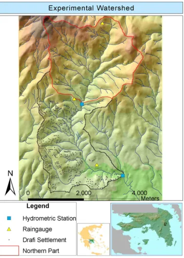
The experimental watershed (Fig. 1) is located at the eastern side of Penteli Moun-tain, in the prefecture of Attica, Greece. The watershed is characterized by pasture areas, in the place of which a thick pine forest existed in the past, more than ten years ago. Attempts of reforestation are being made during the last years. The vegetation type consists mainly of small bushes. A small percentage of inhabited area (Drafi) is 10

included at the southern part of the watershed. The landuses and the corresponding percentages are shown in Table 1.

The total area of the watershed is 15.18 km2, its geometric figure is oblong in the North-South direction and the mean, minimum and maximum altitudes are 430, 146 and 950 m, respectively. The steep slopes constitute another characteristic. The mean 15

slope is equal to 21%.

Geologically, the study area consists approximately of 60% schists, 23% conglom-erates, 9% marls and 8% marbles. The watershed is divided into two parts, north and south, from the geological point of view. The geologic formations that prevail at the northern part are Schist formations with marble intercalations. There is also a small 20

percentage of Marbles with high water capacity, owing to the numerous fractures that have been extended by the karstic process. A karstic aquifer is located at the northeast-ern part, at an altitude zone between 500 and 800 m and is distinguished for its great water potential. It has an excellent diet and contributes significantly to the baseflow of the watershed, which is constant throughout the year.

25

At the southern part of the watershed, there are cohesive conglomeratic formations with varying participation of clay and sand and thus varying infiltration capacity. The

(6)

HESSD

4, 2169–2204, 2007

Initial

Full Screen / Esc

Drafi settlement has been developed on that formation. Additionally, there is a low percentage of impervious marly formations.

The installed equipment consists of two hydrometric stations and a raingauge net-work that has been operating since October 2003. The raingauge netnet-work consists of three gauges that are properly installed in order the complete picture of rainfall to be 5

obtained for the entire watershed. The gauges’ records have a ten-minute time step. The first hydrometric station has been operating since January 2003 and is located at the watershed’s outlet, where stage-discharge measurements are regularly made. The purpose of these measurements is the derivation of the stage-discharge equation, which is used for the transformation of the stage time series into discharge time series. 10

The stream flow measurements at the outlet are accomplished by using a current flow meter. The second hydrometric station (a spillway construction) has been operating since January 2005. It is installed at the outlet of the northern subwatershed, which constitutes about 51% of the extent of the whole watershed. The water level is recorded at ten-minute intervals at both hydrometric stations.

15

The length of the main channel is 7456 m and the density of the channel network is 3.72 km/km2, which implies very good drainage. The baseflow reaches a minimum value (5–15 lt/s) in late summer and a maximum (100–200 lt/s) in spring. The climate at the prefecture of Attica is Mediterranean with a mean annual precipitation of 400 mm and most of the rainfall events occur between October and March.

20

3 Data analysis

3.1 Selection of storm events

Eighteen storm events were selected based on the following criteria: Uniform spatial distribution of the rainfall at the extent of the watershed. Continuous rainfall. Storm events with discontinuous rainfall were excluded. 25

(7)

HESSD

4, 2169–2204, 2007

Initial

Full Screen / Esc

other storm prior to the selected event should have occurred. Summer storm events were excluded.

The winter events at which snowmelt contributed to runoff were also excluded. The peak flow rate of the storm event should be higher than 0.2 m3/s.

The data source was the website: http://www.xbasin.chi.civil.ntua.gr. The analysis 5

time step was thirty minutes. A storm event was considered to be over when there was at least a six-hour period without rainfall. The selected storm events on a rainfall volume ascending order are given in Table 2. The surface rainfall at each event was estimated by the use of the Thiessen Polygon method.

The total excess rainfall Pe in mm was calculated by dividing the total direct runoff 10

volume of each event by the total area of the watershed. The separation of each observed hydrograph into direct runoff and baseflow was based on the hydrograph’s points of inflection. These points indicated the starting and the ending point of direct runoff on the rising and recession limb of each hydrograph, correspondingly.

3.2 SCS method 15

The SCS basic rainfall-runoff equation with the initial abstraction taken into account is the following (SCS, 1972):

P e = (P − Ia)

2

(P − Ia) + S (1)

Where:

P is the total rainfall (mm)

Pe is the total excess rainfall (mm)

Ia is the initial abstraction (mm)

S is the total watershed storage (mm)

The above equation is used when the total rainfall (P) of the storm event is greater 20

than the volume of initial abstraction (P>Ia). In the opposite case, the total excess

rainfall is equal to zero (Pe=0 if P<Ia). The initial abstraction (Ia) consists mainly of

interception, infiltration and surface storage, all of which occur before runoff begins. 2174

(8)

HESSD

4, 2169–2204, 2007

Initial

Full Screen / Esc

The total watershed storage S includes (Ia). Predominantly, S consists of the infiltration

occurring after runoff begins and is controlled by the rate of infiltration at the soil surface or by the rate of transmission in the soil profile or by the water storage capacity of the profile, whichever is the limiting factor (SCS, 1972).

Moreover, the rainfall data that were used for the development of Eq. (1) were totals 5

for one or more storms occurring in a calendar day and nothing was known about the time distributions. The equation therefore excludes time as a variable; this means that rainfall intensity is ignored (SCS, 1972). In addition, Eq. (1) tends to overpredict runoff volume for a discontinuous storm, because it does not account for the recovery of soil storage, caused by infiltration during periods of no rain (Suphunvorranop, 1985). 10

Hjelmfelt (1980b) reports that the SCS method performs better in regions marked by a humid climate if the amount of water retained during runoff is a small fraction of rainfall. The procedure for the determination of the time distribution of excess rainfall, at each storm event, consists of two basic steps:

Firstly, the total excess rainfall (Pe) of the storm event is determined based on the

15

separation of the observed runoff into direct runoff and baseflow. Then, follows the initial abstraction (Ia), which is equal to the accumulated rainfall from the beginning of

the storm to the time when direct runoff starts. The total rainfall (P) of the storm event is known. The only unknown parameter, which is the total watershed storage (S), is calculated using Eq. (1).

20

Secondly, on a thirty-minute time step, the rainfall values of the storm event are accumulated and tabulated. Then, Eq. (1) is used for the calculation of the accumulated excess rainfall value at each time step. Finally, the increment of excess rainfall at each time step is the difference between the accumulated excess rainfall values at the end and the beginning of the time step (Al-Smadi, 1998).

(9)

HESSD

4, 2169–2204, 2007

Initial

Full Screen / Esc

3.2.1 SCS empirical equation

The SCS empirical Equation that relates the initial abstraction Ia with the total storage

S is used in many studies. That is:

I_a_{= 0.2S} ₍₂₎

Equation (2) was derived from records of natural rainfall and runoff from watersheds 5

less than 10 acres in size (one acre is equal to 4046.7 m2), by plotting Ia versus S for

individual storms (SCS, 1972). It is worth mentioning that there was a large amount of scatter in this plotting, mainly because of deficiencies in the accurate estimation of Ia.

Based on recent investigations, Hawkins et al. (2002) suggest changing the coeffi-cient from 0.2 to 0.05. The authors determined the coefficoeffi-cient by two methods for a 10

large number of storms. More than 28 000 storms observed in 307 watersheds located in 24 different eastern states of the United States were used for this purpose. In over 80% of the cases, a value of 0.05 fit the observed rainfall-runoff data better than the original value of 0.2 (Hawkins et al., 2002; Kuntner, 2002).

Substituting Ia from Eq. (2) in Eq. (1), results in the following equation:

15

P e = (P − 0.2S)

2

P + 0.8S (3)

Equation (3) is also used when the total rainfall (P) is greater than the volume of initial abstraction (Ia). (Pe=0 if P<Ia). The procedure for the determination of the time

distri-bution of excess rainfall by using Eq. (3) is the same as above, with the difference that the initial abstraction (Ia) is calculated from Eq. (2) and not from the observed data.

20

3.2.2 SCS infiltration concept

Many questions have arisen regarding the infiltration concept of the SCS method. The SCS method approaches the typical infiltration process, meaning that the estimated losses are greater at the initial time intervals of the storm and they gradually decrease

(10)

HESSD

4, 2169–2204, 2007

Initial

Full Screen / Esc

towards the final, resulting in increasing amounts of excess rainfall. However, the infil-tration model embedded in the SCS method is in disagreement with major infilinfil-tration theories, since the infiltration rate during a storm event of constant rainfall intensity de-creases and approaches zero instead of a residual constant rate resulting in estimated excess rainfall intensity almost equal to the total rainfall intensity. This predicts the 5

excess rainfall at the very end of a storm of low rainfall intensity (Hjelmfelt, 1980a). Smith and Eggert (1978) point out two major disagreements of the SCS method with other infiltration theories. The first is that the infiltration, before runoff starts, has a uniform value Ia. Second, according to the SCS method, the infiltration rate, after runoff

starts, depends on rainfall rate. In reality, however, the first phase is not a uniform value 10

and the length of it depends on the rainfall rate and patterns, because the surface flux capacity, provided by the soils unsaturated capillary gradient, is larger than the rainfall rate. In the second phase, the rainfall rate surpasses the infiltration capacity and the infiltration rate is controlled only by the condition of the soil (Smith and Eggert, 1978; Brevnova, 2001). Meadows and Chestnut (1983) conclude that the infiltration model 15

embedded in the SCS method performs well only when the rainfall events considered are of short duration without interruptions or for longer lasting periods of rainfall where the soil saturated hydraulic conductivity is not exceeded.

4 Results and discussion

4.1 Determination of the initial abstraction Ia– storage S ratio

20

The procedure for the determination of the ratio (Ia/S) at each one of the storm events

was the following: first, the total excess rainfall (Pe) at each event was estimated from

the observed direct runoff. Then, the initial abstraction was determined from the ob-served rainfall-runoff data. At the next step, the total storage S of the watershed, for that event, was calculated by the use of Eq. (1).

25

(11)

HESSD

4, 2169–2204, 2007

Initial

Full Screen / Esc

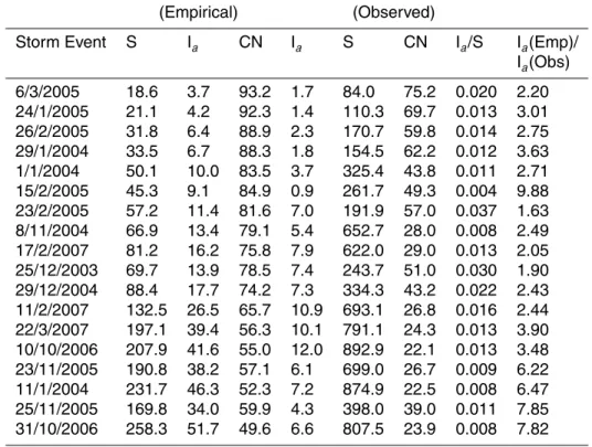
of the watershed is equal to 0.014. The maximum value was 0.037 and the minimum 0.004. More specifically, the results that were calculated for each storm event are shown in Table 3. In this table, the empirical Eq. (2) was taken into account for the calculations in the first three columns, while in the next columns the initial abstraction was determined from the observed rainfall-runoff data.

5

The ratio Ia(Emp)/Ia(Obs), which shows how many times one is bigger than the other,

varied from 1.63 to 9.88 and it increased with the increase in rainfall. The CN was calculated from the following equation:

CN = 25400

S + 254 (4)

Where: S is the total storage of the watershed in mm. 10

The values of Iaand S for each event are plotted in Fig. 2 and the values of the ratio

(Ia/S) versus the runoff coefficient at each storm event are plotted in Fig. 3. Figure 2

shows that the initial abstraction, determined from the observed data, is proportional to the total watershed storage at each event, while Fig. 3 shows that the ratio (Ia/S) at

most of the events is around 0.01 and is not related to the runoff coefficient. 15

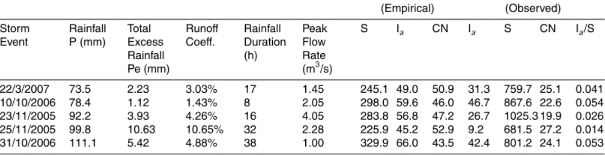
Additionally, for comparison reasons, a research into the values of the ratio (Ia/S) was

conducted at the northern subwatershed. Five storm events were selected based on the same criteria as above, plus the criterion that the rainfall volume of each storm event should be higher than 20 mm, since lower rainfall produces insignificant hydrograph at the outlet of the northern subwatershed.

20

The selected storm events, which occurred after January 2005, and the results of the analysis are shown in Table 4. The ratio (Ia/S) varied from 0.014 to 0.054 and

the average value was 0.037. Despite the fact that more events are necessary for the analysis at the northern part, the determined values indicate a higher ratio.

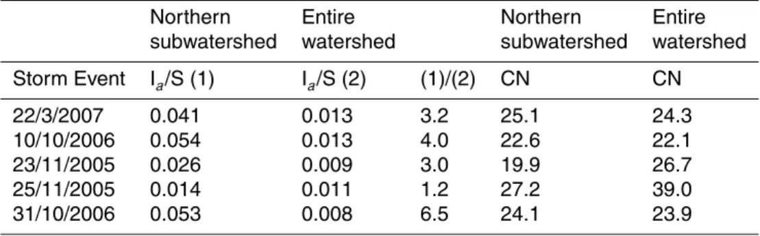
A comparison between the ratios was also done for the five common storm events 25

and is shown in Table 5. The ratio that was determined at the northern subwatershed is about 3–4 times the ratio of the entire watershed. The calculated CN values for the

(12)

HESSD

4, 2169–2204, 2007

Initial

Full Screen / Esc

northern subwatershed and the entire watershed are low, but consistent, approximately equal to 24.

The graph of total rainfall P versus total watershed storage S, at each storm event, is depicted in Fig. 4. The storage S was calculated by Eq. (1) in the first series of points, denoting that the initial abstraction was determined from the observed rainfall-runoff 5

data. The storage S was calculated by Eq. (3) in the second series of points, denoting that the empirical Eq. (2) was taken into account for the calculation of initial abstraction. The graph shows that the rainfall and the storage are proportionally related. Once the rainfall volume increases the total watershed storage also increases. Comparing the estimated values of storage, the values are much greater in the case of use of the 10

observed rainfall-runoff data, leading to lower CN values.

The determined low ratio (Ia/S) and the great storage of the watershed, which

in-creases proportionally to rainfall, are attributed to the combination of the geological and landcover characteristics of the watershed.

The great storage is owed to the special geological structure in combination with the 15

fact that the formations of the whole area are tectonically intensely folded. Schist for-mations with marble intercalations dominate the northern part of the watershed. They constitute about 85% of the area of this part. These formations are normally imper-vious when they are at a healthy condition. However, in our case, their upper layer is corroded resulting in the interception of water. Moreover, there are major marble forma-20

tions, intensely karstic, constituting about 15% of the northern part of the watershed. These formations are characterized by very low runoff coefficient. The southern part of the watershed is more complicated. It consists of a great percentage of impervious areas (residencies, roads), which is constantly increasing due to the high growth rates of the inhabited area of Drafi settlement. Moreover, there are cohesive conglomer-25

atic formations with varying participation of clay and sand and nearly impervious marly formations.

Additionally, the landcover that is dominated by pasture areas (about 88% of the watershed’s total area) plays an important role in the retention of rainfall, as well as in

(13)

HESSD

4, 2169–2204, 2007

Initial

Full Screen / Esc

the interception of water due to the decrease in the surface water velocity.

The low ratio (Ia/S) of the watershed is mainly attributed to the impervious areas of

the southern part. The residencies and the road surfaces of the inhabited area of Drafi constitute areas characterized by high runoff coefficient. The runoff from these areas reaches quickly at the outlet of the watershed, contributing to the quick start of direct 5

runoff, at the early stages of the storm. Thus, the amount of initial abstraction of the watershed is low. The higher ratio (Ia/S) at the northern subwatershed is owed to the

lack of impervious areas that implies greater amounts of initial abstraction. 4.2 Effect of the SCS empirical equation on hydrograph simulation

Two simulated hydrographs were calculated for each storm event and resulted from 10

the following process: Firstly, two time distributions of excess rainfall were estimated at each storm event by two different approaches.

Regarding the first approach, which is called SCS(1), the initial abstraction was de-termined at each storm from the observed rainfall-runoff data, since it is equal to the accumulated rainfall from the beginning of the storm to the time when runoff started. 15

Then, Eq. (1) was used for the estimation of the time distribution of excess rainfall. This time distribution is denoted as “Rainfall Excess 1” in the legend of the rainfall-runoff graphs.

In the second approach, which is called SCS(2), Eq. (2) was used for the calculation of initial abstraction. Then, the excess rainfall time distribution was estimated by Eq. (3). 20

This time distribution is denoted as ‘’Rainfall Excess 2” in the legend of the rainfall-runoff graphs.

The two estimated time distributions of excess rainfall were applied on the unit hy-drograph of the watershed and two different simulated hyhy-drographs were derived. The simulated hydrographs that resulted from the “Rainfall Excess 1” and “Rainfall Excess 25

2” time distributions are called “Runoff Sim1” and “Runoff Sim2”, correspondingly, in the rainfall-runoff graphs. These two simulated hydrographs were compared with the observed hydrograph, at each storm event, focusing on the values of peak flow rate

(14)

HESSD

4, 2169–2204, 2007

Initial

Full Screen / Esc

and time to peak flow rate. The time to peak flow rate is defined as the time period from the beginning of rainfall to the time point of peak flow rate.

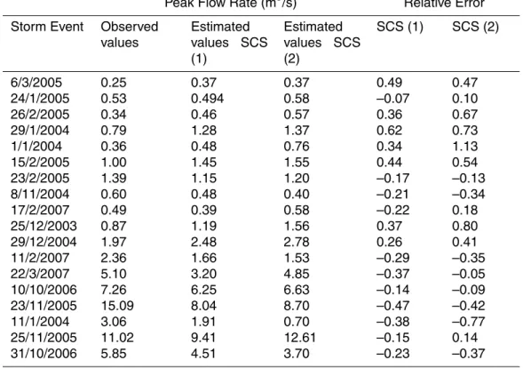
The observed and the estimated values of peak flow rate, as well as the relative errors in the peak flow rate for all the storm events are shown in Table 6. At 61% of the events the estimations of the SCS(1) method produced negative relative error, while 5

the corresponding percentage for the SCS(2) was 44%. Both of the estimated values from the two methods approached the observed, but the estimations of the SCS(2) method were generally higher than those of the SCS(1) with the exception at three out of the eighteen events.

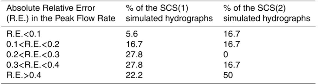
The absolute relative error in the peak flow rate was calculated for each event and 10

the results were categorized, as shown in Table 7. The average relative error in the peak flow rate, which is the average of the absolute values, was 0.31 for the SCS(1) method versus 0.43 for the SCS(2) method.

Overall, the empirical Eq. (2) overestimated the initial abstraction at each storm event and led to the delay in the beginning of excess rainfall. Therefore, the total excess rain-15

fall at each event had to be allocated in a shorter time period, resulting in overestimated excess rainfall values and consequently, overestimated flow rates.

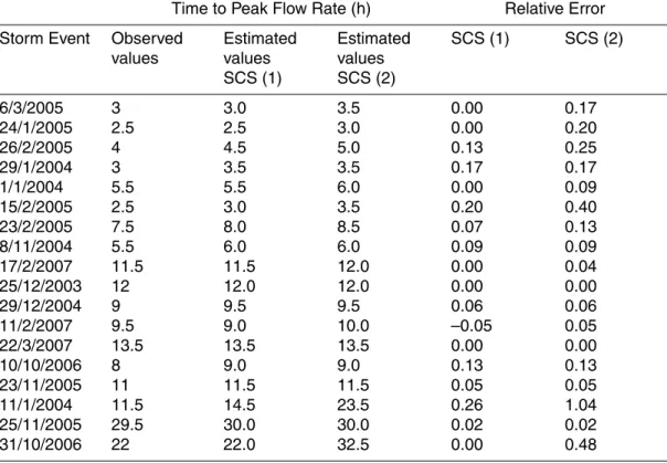
Regarding the estimations in the time to peak, the estimated values and the relative errors in the time to peak flow rate for all the storm events are shown in Table 8. All the estimated values were greater than the observed. Comparing the estimated values 20

from the two methods, at 39% of the storm events the values estimated by the SCS(2) method were half an hour greater than those estimated by the SCS(1) method. At 17% of the events the differences in the estimations were greater than one hour. At the rest 44% of the storm events the estimated values of the time to peak were exactly the same.

25

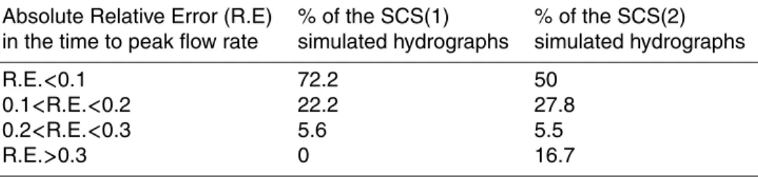
The absolute relative error in the time to peak flow rate was calculated for each storm event and the results were categorized, as shown in Table 9. The average relative error in the time to peak flow rate was 0.067 for the SCS(1) method versus 0.187 for the SCS(2) method. The reason for the greater estimations in the time to peak values

(15)

HESSD

4, 2169–2204, 2007

Initial

Full Screen / Esc

from the SCS(2) method is the same as above. The delay in the beginning of excess rainfall due to the greater amounts of initial abstraction that were determined from the empirical equation, results in a short time displacement, towards greater values, of the simulated time to peak.

Regarding the general shape of the hydrographs, at short-duration storm events 5

(Fig. 5 – storm of 1 January 2004, Fig. 6 – storm of 26 February 2005) with great fluctuations in rainfall intensity and more than one peak flow rate, the simulated runoff did not approach satisfactorily the shape of the observed. On the contrary, at long-duration storms, (Fig. 7 – storm of 25 November 2005, Fig. 8 – storm of 31 October 2006, Fig. 9 – storm of 17 February 2007) the simulated hydrographs, especially those 10

of the SCS(1), approached more closely the fluctuations of the observed hydrographs. This is owed to the fact that the initial abstraction exerts a stronger influence on the time distribution of excess rainfall at short-duration events.

Moreover, low-intensity rainfall intervals at the end of some storms (Fig. 10 – storm of 23 November 2005, Fig. 11 – storm of 8 November 2004) produced overestimated 15

flow rates that exceeded the observed. This is owed to the general SCS infiltration concept that estimates greater amounts of excess rainfall as the duration of the storm increases.

5 Conclusions

The low (0.014) average initial abstraction Ia– storage S ratio of the entire watershed is

20

attributed to its great storage in combination with the low amount of initial abstraction. The later is owed to the impervious areas of Drafi settlement, located at the southern part, that contribute to runoff at the early stages of the storm. The storage of the wa-tershed is attributed to its special geological structure, which results in the interception of water, in combination with the great percentage of pasture areas that contribute to 25

the retention of rainfall. The average ratio (Ia/S) is greater (0.037) at the northern

sub-watershed, due to the lack of impervious areas that generate early runoff. Thus, the 2182

(16)

HESSD

4, 2169–2204, 2007

Initial

Full Screen / Esc

initial abstraction is higher, leading to higher (Ia/S) ratio.

The SCS empirical Eq. (2) that was used in the SCS(2) method, consistently over-estimated the initial abstraction in all of the storm events. It was approximately 2 to 4 times the one determined from the observed rainfall-runoff data. This resulted in the delayed start of excess rainfall and consequently in the delayed start of the simulated 5

runoff. The total excess rainfall volume at each storm event had to be allocated in a shorter time period, leading to overestimated excess rainfall values and consequently, overestimated peak flow rate in the resulting simulated hydrographs. Regarding the estimated time to peak values, the use of the SCS empirical equation also led to over-estimations for the same reason.

10

References

Al-Smadi, M.: Incorporating spatial and temporal variation of watershed response in a Gis-based hydrologic model, MS thesis, Faculty of the Virginia Polytechnic Institute and State University, Blacksburg, 1998.

Brevnova, E. V.: Green-Ampt Infiltration Model Parameter Determination Using SCS Curve

15

Number (CN) and Soil Texture Class, and Application to the SCS Runoff Model, Master Thesis, Department of Civil and Environmental Engineering, Morgantown, West Virginia, 2001.

Dervos, N. A., Baltas, E. A., and Mimikou, M. A.: Rainfall–runoff simulation in an experimental basin using GIS methods, J. Environ. Hydrol., 14, 2006.

20

Hawkins, R. H., Jiang, R., Woodward, D. E., Hjelmfelt, A. T., and Van Mullem, J. A.: Runoff Curve Number Method: Examination of the Initial Abstraction Ratio. In: Proceedings of the Second Federal Interagency Hydrologic Modeling Conference, Las Vegas, Nevada. U.S. Ge-ological Survey, Lakewood, Colorado, 2002.

Hjelmfelt, A. T.: Curve Number Procedure as Infiltration Method, J. Hydraulics Division, ASCE,

25

106, 1107–1111, 1980a.

Hjelmfelt, A. T.: Empirical investigation of Curve Number technique, J. Hydraulics Division, 106, 1471–1476, 1980b.

(17)

HESSD

4, 2169–2204, 2007

Initial

Full Screen / Esc

Interactive Discussion model. MS thesis, Biological Systems Engineering Dept., Faculty of the Virginia Polytechnic

Institute and State University, Blacksburg, 1997.

Kuntner, R.: A Methodological Framework towards the formulation of flood runoff generation models suitable in Alpine and Prealpine regions. Dissertation, Swiss Federal Institute of Technology, Z ¨urich, 2002.

5

Meadows, M. E. and Chestnut, A. L.: The Curve Number runoff model as an infiltration model for hydrograph simulation. Proceedings of the specialty conference on advances in irrigation and drainage: Surviving external pressures. Jackson. Wyoming, 299–307, 1983.

SCS.: National Engineering Handbook, Section 4: Hydrology. Chapter 10: Estimation of direct runoff from storm rainfall by Victor Mockus, 1972.

10

Smith, R. E. and Eggert K. G.: Discussion of “Infiltration Formula Based on SCS Curve Num-ber”, edited by: Aron, G., Miller, A. C., and Lakatos,D. F., J. Irrigation and Drainage Division, ASCE, 104(4), 462–64, 1978.

Suphunvorranop, T.: Technical Publication No. 85-5. A guide to SCS runoff procedures, Department of Water Resources, St. Johns River Water Management District, Palatka,

15

Florida,1985.

Website of the experimental watershed:http://www.xbasin.chi.civil.ntua.gr.

(18)

HESSD

4, 2169–2204, 2007

Initial

Full Screen / Esc

Table 1. The landuses of the experimental watershed.

Landuse Area (m2) Percentage % Pasture 10 541 581 70.2

Wood 113 247 0.75

Inhabited area (Drafi)

1.Residencies 1 118 250 7.37 2.Roads (impervious surface) 502 394 3.3 3.Pasture among residencies 2 791 013 18.38

(19)

HESSD

4, 2169–2204, 2007

Initial

Full Screen / Esc

Table 2. Selected storm events.

Total Peak

A/A Storm Event Rainfall Excess Runoff Rainfall Flow P (mm) Rainfall Coefficient Duration Rate Pe (mm) (h) (m3/s) 1 6/3/2005 5.60 0.17 3.11% 9.5 0.25 2 24/1/2005 6.53 0.23 3.49% 2.5 0.53 3 26/2/2005 9.59 0.30 3.11% 5.5 0.34 4 29/1/2004 11.22 0.54 4.78% 3.0 0.79 5 1/1/2004 14.26 0.33 2.33% 7.0 0.36 6 15/2/2005 15.23 0.74 4.87% 5.0 1.00 7 23/2/2005 17.05 0.50 2.93% 8.0 1.39 8 8/11/2004 17.26 0.21 1.23% 9.0 0.60 9 17/2/2007 21.09 0.27 1.3% 12 0.49 10 25/12/2003 21.92 0.82 3.75% 6.0 0.87 11 29/12/2004 29.44 1.38 4.68% 11.5 1.97 12 11/2/2007 39.20 1.11 2.84% 11.5 2.36 13 22/3/2007 70.93 4.34 6.12% 17.0 5.10 14 10/10/2006 71.11 3.67 5.17% 10.0 7.26 15 23/11/2005 76.66 6.46 8.43% 16.0 15.09 16 11/1/2004 91.84 7.47 8.14% 32.0 3.06 17 25/11/2005 100.37 18.67 18.60% 33 11.02 18 31/10/2006 117.58 13.41 11.40% 38.0 5.85 2186

(20)

HESSD

4, 2169–2204, 2007

Initial

Full Screen / Esc

Table 3. Relationship between initial abstraction Iaand storage S of the watershed. The storage S was calculated by Eq. (3) in the first column and then, Iaand CN from S. The storage S was

calculated by Eq. (1) in the fifth column, after having determined Iafrom the observed data.

(Empirical) (Observed)

Storm Event S Ia CN Ia S CN Ia/S Ia(Emp)/

Ia(Obs) 6/3/2005 18.6 3.7 93.2 1.7 84.0 75.2 0.020 2.20 24/1/2005 21.1 4.2 92.3 1.4 110.3 69.7 0.013 3.01 26/2/2005 31.8 6.4 88.9 2.3 170.7 59.8 0.014 2.75 29/1/2004 33.5 6.7 88.3 1.8 154.5 62.2 0.012 3.63 1/1/2004 50.1 10.0 83.5 3.7 325.4 43.8 0.011 2.71 15/2/2005 45.3 9.1 84.9 0.9 261.7 49.3 0.004 9.88 23/2/2005 57.2 11.4 81.6 7.0 191.9 57.0 0.037 1.63 8/11/2004 66.9 13.4 79.1 5.4 652.7 28.0 0.008 2.49 17/2/2007 81.2 16.2 75.8 7.9 622.0 29.0 0.013 2.05 25/12/2003 69.7 13.9 78.5 7.4 243.7 51.0 0.030 1.90 29/12/2004 88.4 17.7 74.2 7.3 334.3 43.2 0.022 2.43 11/2/2007 132.5 26.5 65.7 10.9 693.1 26.8 0.016 2.44 22/3/2007 197.1 39.4 56.3 10.1 791.1 24.3 0.013 3.90 10/10/2006 207.9 41.6 55.0 12.0 892.9 22.1 0.013 3.48 23/11/2005 190.8 38.2 57.1 6.1 699.0 26.7 0.009 6.22 11/1/2004 231.7 46.3 52.3 7.2 874.9 22.5 0.008 6.47 25/11/2005 169.8 34.0 59.9 4.3 398.0 39.0 0.011 7.85 31/10/2006 258.3 51.7 49.6 6.6 807.5 23.9 0.008 7.82

(21)

HESSD

4, 2169–2204, 2007

Initial

Full Screen / Esc

Table 4. Initial abstraction – storage ratio at the northern subwatershed.

(Empirical) (Observed) Storm Event Rainfall P (mm) Total Excess Rainfall Pe (mm) Runoff Coeff. Rainfall Duration (h) Peak Flow Rate (m3/s) S Ia CN Ia S CN Ia/S 22/3/2007 73.5 2.23 3.03% 17 1.45 245.1 49.0 50.9 31.3 759.7 25.1 0.041 10/10/2006 78.4 1.12 1.43% 8 2.05 298.0 59.6 46.0 46.7 867.6 22.6 0.054 23/11/2005 92.2 3.93 4.26% 16 4.05 283.8 56.8 47.2 26.7 1025.3 19.9 0.026 25/11/2005 99.8 10.63 10.65% 32 2.28 225.9 45.2 52.9 9.2 681.5 27.2 0.014 31/10/2006 111.1 5.42 4.88% 38 1.00 329.9 66.0 43.5 42.4 801.2 24.1 0.053 2188

(22)

HESSD

4, 2169–2204, 2007

Initial

Full Screen / Esc

Table 5. Comparison between the ratios (Ia/S) at the northern subwatershed and the entire watershed.

Northern Entire Northern Entire subwatershed watershed subwatershed watershed Storm Event Ia/S (1) Ia/S (2) (1)/(2) CN CN 22/3/2007 0.041 0.013 3.2 25.1 24.3 10/10/2006 0.054 0.013 4.0 22.6 22.1 23/11/2005 0.026 0.009 3.0 19.9 26.7 25/11/2005 0.014 0.011 1.2 27.2 39.0 31/10/2006 0.053 0.008 6.5 24.1 23.9

(23)

HESSD

4, 2169–2204, 2007

Initial

Full Screen / Esc

Table 6. Peak flow rate analysis.

Peak Flow Rate (m3/s) Relative Error Storm Event Observed

values Estimated values SCS (1) Estimated values SCS (2) SCS (1) SCS (2) 6/3/2005 0.25 0.37 0.37 0.49 0.47 24/1/2005 0.53 0.494 0.58 –0.07 0.10 26/2/2005 0.34 0.46 0.57 0.36 0.67 29/1/2004 0.79 1.28 1.37 0.62 0.73 1/1/2004 0.36 0.48 0.76 0.34 1.13 15/2/2005 1.00 1.45 1.55 0.44 0.54 23/2/2005 1.39 1.15 1.20 –0.17 –0.13 8/11/2004 0.60 0.48 0.40 –0.21 –0.34 17/2/2007 0.49 0.39 0.58 –0.22 0.18 25/12/2003 0.87 1.19 1.56 0.37 0.80 29/12/2004 1.97 2.48 2.78 0.26 0.41 11/2/2007 2.36 1.66 1.53 –0.29 –0.35 22/3/2007 5.10 3.20 4.85 –0.37 –0.05 10/10/2006 7.26 6.25 6.63 –0.14 –0.09 23/11/2005 15.09 8.04 8.70 –0.47 –0.42 11/1/2004 3.06 1.91 0.70 –0.38 –0.77 25/11/2005 11.02 9.41 12.61 –0.15 0.14 31/10/2006 5.85 4.51 3.70 –0.23 –0.37 2190

(24)

HESSD

4, 2169–2204, 2007

Initial

Full Screen / Esc

Table 7. Absolute relative error in the peak flow rate.

Absolute Relative Error % of the SCS(1) % of the SCS(2) (R.E.) in the Peak Flow Rate simulated hydrographs simulated hydrographs

R.E.<0.1 5.6 16.7

0.1<R.E.<0.2 16.7 16.7 0.2<R.E.<0.3 27.8 0 0.3<R.E.<0.4 27.8 16.7

(25)

HESSD

4, 2169–2204, 2007

Initial

Full Screen / Esc

Table 8. Time to peak flow rate analysis.

Time to Peak Flow Rate (h) Relative Error Storm Event Observed

values Estimated values SCS (1) Estimated values SCS (2) SCS (1) SCS (2) 6/3/2005 3 3.0 3.5 0.00 0.17 24/1/2005 2.5 2.5 3.0 0.00 0.20 26/2/2005 4 4.5 5.0 0.13 0.25 29/1/2004 3 3.5 3.5 0.17 0.17 1/1/2004 5.5 5.5 6.0 0.00 0.09 15/2/2005 2.5 3.0 3.5 0.20 0.40 23/2/2005 7.5 8.0 8.5 0.07 0.13 8/11/2004 5.5 6.0 6.0 0.09 0.09 17/2/2007 11.5 11.5 12.0 0.00 0.04 25/12/2003 12 12.0 12.0 0.00 0.00 29/12/2004 9 9.5 9.5 0.06 0.06 11/2/2007 9.5 9.0 10.0 –0.05 0.05 22/3/2007 13.5 13.5 13.5 0.00 0.00 10/10/2006 8 9.0 9.0 0.13 0.13 23/11/2005 11 11.5 11.5 0.05 0.05 11/1/2004 11.5 14.5 23.5 0.26 1.04 25/11/2005 29.5 30.0 30.0 0.02 0.02 31/10/2006 22 22.0 32.5 0.00 0.48 2192

(26)

HESSD

4, 2169–2204, 2007

Initial

Full Screen / Esc

Table 9. Absolute relative error in the time to peak flow rate.

Absolute Relative Error (R.E) % of the SCS(1) % of the SCS(2) in the time to peak flow rate simulated hydrographs simulated hydrographs

R.E.<0.1 72.2 50

0.1<R.E.<0.2 22.2 27.8 0.2<R.E.<0.3 5.6 5.5

(27)

HESSD

4, 2169–2204, 2007

Initial

Full Screen / Esc

Fig. 1. The study area.

(28)

HESSD

4, 2169–2204, 2007

Initial

Full Screen / Esc

(29)

HESSD

4, 2169–2204, 2007

Initial

Full Screen / Esc

Fig. 3. Graph of the (Ia/S) ratio versus runoff coefficient, at each event.

(30)

HESSD

4, 2169–2204, 2007

Initial

Full Screen / Esc

Fig. 4. Graph of total rainfall P versus total watershed storage S, at each storm event.

Equa-tion (1) takes into account the observed data for the determinaEqua-tion of initial abstracEqua-tion, while in Eq. (3) the initial abstraction is calculated from the SCS empirical equation.

(31)