Mid-latitude ozone changes: studies with a 3-D CTM forced by ERA-40 analyses

(1)

HAL Id: hal-00301989

https://hal.archives-ouvertes.fr/hal-00301989

Submitted on 17 Jul 2006

HAL is a multi-disciplinary open access

archive for the deposit and dissemination of sci-entific research documents, whether they are pub-lished or not. The documents may come from teaching and research institutions in France or abroad, or from public or private research centers.

L’archive ouverte pluridisciplinaire HAL, est destinée au dépôt et à la diffusion de documents scientifiques de niveau recherche, publiés ou non, émanant des établissements d’enseignement et de recherche français ou étrangers, des laboratoires publics ou privés.

Mid-latitude ozone changes: studies with a 3-D CTM

forced by ERA-40 analyses

W. Feng, M. P. Chipperfield, M. Dorf, K. Pfeilsticker

To cite this version:

W. Feng, M. P. Chipperfield, M. Dorf, K. Pfeilsticker. Mid-latitude ozone changes: studies with a 3-D CTM forced by ERA-40 analyses. Atmospheric Chemistry and Physics Discussions, European Geosciences Union, 2006, 6 (4), pp.6695-6722. �hal-00301989�

(2)

ACPD

6, 6695–6722, 2006 Mid-latitude ozone changes in a 3-D CTM W. Feng et al. Title Page Abstract Introduction Conclusions References Tables Figures J I J I Back Close

Full Screen / Esc

Printer-friendly Version Interactive Discussion

EGU Atmos. Chem. Phys. Discuss., 6, 6695–6722, 2006

www.atmos-chem-phys-discuss.net/6/6695/2006/ © Author(s) 2006. This work is licensed

under a Creative Commons License.

Atmospheric Chemistry and Physics Discussions

Mid-latitude ozone changes: studies with

a 3-D CTM forced by ERA-40 analyses

W. Feng1, M. P. Chipperfield1, M. Dorf2, and K. Pfeilsticker2

1

Institute for Atmospheric Science, School of Earth and Environment, University of Leeds, Leeds, UK

2

Institute f ¨ur Umweltphysik, University of Heidelberg, Heidelberg, Germany Received: 3 April 2006 – Accepted: 21 April 2006 – Published: 17 July 2006 Correspondence to: M. P. Chipperfield (martyn@env.leeds.ac.uk)

(3)

ACPD

Full Screen / Esc

EGU

Abstract

We have used an off-line three-dimensional (3-D) chemical transport model (CTM) to study long-term changes in stratospheric O₃. The model was run from 1977–2004 and forced by ECMWF ERA-40 and operational analyses. Model runs were performed to examine the impact of increasing halogens and additional stratospheric bromine from

5

short-lived source gases. The analyses capture much of the observed interannual variability in column ozone, but there are also unrealistic features. In particular the ERA-40 analyses cause a large positive anomaly in northern hemisphere (NH) column O₃in the late 1980s. Also, the change from ERA-40 to operational winds at the start of 2002 introduces abrupt changes in some model fields which affect analysis of trends.

10

The model reproduces the observed column increase in NH mid-latitudes from the mid 1990s. Analysis of a run with fixed halogens shows that this increase is not due to a significant decrease in halogen-induced loss, i.e. is not an indication of recovery. The model predicts only a small decrease in halogen-induced loss after 1999. In the upper stratosphere, despite the modelled turnover of chlorine around 1999, O₃ does

15

not increase to the effects of increasing ECMWF temperatures, decreasing modelled CH₄ at this altitude, and abrupt changes to the SH temperatures at the end of the ERA-40 period. The impact of an additional 5 pptv stratospheric bromine from short-lived species decreases mid-latitude column O₃by about 10 DU. However, the impact on the modelled relative O₃ anomaly is generally small except during periods of large

20

volcanic loading.

1 Introduction

A quantitative explanation of the observed changes in mid-latitude column ozone has still not been achieved. Although the likely contributing processes have been identified (e.g. see WMO, 2003) their relative importance is still not clear. These processes

25

(4)

ACPD

Full Screen / Esc

EGU is that all of the different processes have not been brought together in a single long-term

model study. In addition, changes in the observed variations mean that the separation of “trend” from long-term “variability” depends on the period considered, i.e. the relative importance of processes to the apparent trend will change as the length of time series changes.

5

In a series of papers Hadjinicolaou and co-workers have studied the influence of dynamics on northern hemisphere (NH) column ozone using an off-line 3-D transport model (SLIMCAT) forced by ECMWF analyses. Hadjinicolaou et al. (2002) ran the model from 1979–1998 using analyses with a top lid at 10 hPa and showed that the model captured many observed variations in NH column ozone. Recently,

Hadjinico-10

laou et al. (2005) have performed a similar CTM study from 1957–2003 using analyses which extend to 0.1 hPa (ERA-40 until 2001 and then operational). This study again showed that the model captured alot of the observed NH column ozone variability and, interestingly, the model reproduced the observed increase in NH column ozone after the mid 1990s.

15

Chipperfield (2003) used a similar model set-up to Hadjinicolaou et al. (2002) but with detailed stratospheric chemistry to perform long-term simulations. He cautioned that the modelled dynamical variability in the 1990s, when the model was forced by operational analyses, did not match the observations well. Nevertheless, by running the model with time-dependent and fixed halogen loadings he argued that halogen

20

changes did dominate the observed trends from 1980 until the early 1990s. However, the vertical extent of the ERA-15 analyses, and their short time period, limited this study. Recently, Stolarski et al. (2006) used a full chemistry CTM, forced by winds from a general circulation model, to investigate ozone trends. They found that their model, which included observed changes in halogens and aerosol, was able to reproduce

25

much of the long term globally average variations in column ozone over the past 20 years.

Recently, the bromine loading of the stratosphere has received alot of attention. Many past studies (e.g. Sinnhuber et al., 2002) have used BrO observations to infer

(5)

ACPD

Full Screen / Esc

EGU that the inorganic bromine (Br_y) loading of the stratosphere is currently around 21 pptv.

Salawitch et al. (2005) discussed the stratosphere bromine budget and showed that this inferred Br_y loading is greater than that delivered by long-lived organic source gases by between 4–8 pptv. This discrepancy can be accounted for by contributions from short-lived bromine source gases. The study by Salawitch et al. (2005) included

5

2-D (latitude-height) model calculations of the impact of this extra 4–8 pptv on NH mid-latitude column O₃. This additional Br_y increased the modelled O₃loss, notably around the time of the large aerosol loading from Mt. Pinatubo in the early 1990s. However, 2-D models cannot be expected to capture the interaction of polar loss with mid-latitudes realistically.

10

Past model studies have sometimes based their bromine loading solely on the long-lived species (e.g. WMO, 2003) in which cases the model will fall short of the observed loading by around 6 pptv, and the model will underestimate the impact of bromine chemistry on O₃. Other studies (e.g. Chipperfield, 1999) have assumed a more re-alistic loading of ∼20 pptv by increasing the model abundance of a long-lived source

15

gas to account for the short-lived species not explicitly included in the model. This approach is reasonable for most of the stratosphere but discrepancies in Br_ymight be expected in young air in the lower stratosphere.

In this paper we have used the SLIMCAT 3-D off-line chemical transport model (CTM) with a detailed stratospheric chemistry scheme to perform full-stratosphere decadel

in-20

tegrations. We examine the role of chemical processes on mid-latitude ozone changes and the effect of bromine from short-lived substances. This paper is therefore an up-date of Chipperfield (2003) with longer-term, full stratosphere simulations using ERA-40 analyses. It revisits some issues raised in the northern hemisphere (NH) study of Hadjinicolaou et al. (2005) using a model with a full chemistry scheme. Finally, we add

25

to the bromine study of Salawitch et al. (2005) by using a full 3-D model. Section 2 de-scribes the model and experiments. Section 3 discusses the model results and Sect. 4 summarises our conclusions.

(6)

ACPD

Full Screen / Esc

EGU

2 Model and experiments

2.1 SLIMCAT 3-D CTM

SLIMCAT is an off-line 3-D CTM described in detail by Chipperfield (1999). The model has been used in many past studies of stratospheric chemistry and shown to perform well at simulating key chemistry and transport processes. The model uses a hybrid

5

σ-θ vertical coordinate (Chipperfield, 2006) and extends from the surface to a top level

which depends on the domain of the forcing analyses. Vertical advection in the θ-level domain is calculated from diabatic heating rates using a radiation scheme which gives a better representation of vertical transport and age-of-air even with ERA-40 analyses (Chipperfield, 2006). The model contains a detailed stratospheric chemistry

10

scheme including a treatment of heterogeneous reactions on liquid aerosols, nitric acid trihydrate (NAT) and ice (see Chipperfield, 1999). The current details of the chemistry scheme are as described in Feng et al. (2005).

For the runs described here two extra tracers for bromine source gases have been added to the model. These represent a halon and a very short-lived species (VSLS)

15

and were set up using the photochemical data for H1211 and CH₂Br₂ respectively. In the model experiments the surface mixing ratios of these tracers are set to the total val-ues of all halon species and a constant 4 pptv respectively. In addition, the tropospheric Br_y mixing ratio was set at 1 pptv.

In the experiments described here the 3-D model resolution was 7.5◦×7.5◦ with

20

24 levels from the surface to approximately 60 km. The model was forced using the 6-hourly 60-level European Centre for Medium-Range Weather Forecasts (ECMWF) analyses. From 1 January 1977 to 31 December 2001 we have used the standard “ERA-40” product (Uppala et al., 2005). After this date we have used the operational analyses which are subject to periodic update. Time-dependent monthly fields of

liq-25

uid sulfate aerosol for 1979–1999 were taken from WMO (2003). When the model simulations extended beyond 1999 the aerosol was kept constant at the 1999 values. The time-dependent surface mixing ratios of source gases were also taken from WMO

(7)

ACPD

Full Screen / Esc

EGU (2003).

The model was initialised on 1 January 1977 using output from a 2-D model and integrated until 2004 in a series of experiments (see Table 1). Run A used the basic model and time-dependent values for the halogen loading and aerosols. Run B was similar to A but used a tropospheric halogen loading fixed at 1979 values. Run C was

5

similar to A but did not include the contribution of bromine from the VSLS tracer nor the direct input of Br_y from the troposphere, i.e. the total bromine loading was 5 pptv less than run A. Finally, run D was similar to A except that all of the model tropospheric bromine was put into the form of CH₃Br to mimic the approach used in older SLIMCAT studies (e.g. Chipperfield, 1999, 2003).

10

3 Results

3.1 Bromine loading

Figure1shows an example of observed BrO profiles from Kiruna (67◦N) on 24 March 2004 using the University of Heidelberg balloon-borne DOAS instrument (e.g. Dorf et al. 2005). DOAS BrO measurements indicate that at present the inorganic bromine

15

(Br_y) loading in the stratsphere is around 21 pptv and therefore 4–5 pptv higher than the known organic precusors, halons and CH₃Br (around 16.5 pptv in 5 year old air, see Montzka et al. 2003), can account for. Detailed model comparisons (Dorf 2005) reveal that the major part of this discrepancy is due to short-lived organic bromine species (VSLS) and their injection into the stratosphere. Direct injection of tropospheric

inor-20

ganic bromine into the stratosphere possibly also contributes to a lesser extent (around 1 pptv). The fast release of Br_y and the rapid increase of BrO above the tropopause can particularly be observed for the tropical measurements at Teresina (see Dorf et al. 20061) but the difference is also present at high latitudes.

1

Dorf, M., B ¨osch, H., Butz, A., Camy-Peret, C., Chipperfield, M. P., Grunow, K., Harder, H., Kritten, L., Payan, S., Simmes, B., Weidner, F., and Pfeilsticker, K.: Comparison of measured

(8)

ACPD

Full Screen / Esc

EGU Also shown in Fig. 1 are profiles of bromine species from the basic model run (A)

and the run which mimics our former treatment of all tropospheric bromine released as CH₃Br (D). Although the overall bromine loading is set to be the same (around 21 pptv during this period) run A has a larger mixing ratio of Br below ∼25 km through non-zero tropospheric Br and faster overall release of bromine from its source gases. This

5

leads to around 1–2 pptv more BrO between 15–25 km which gives better agreement with these balloon flights. A discussion of other flights, which confirm the improved agreement of run A is given in Dorf et al. (2006)1. Clearly, the model run C, which does not consider the 5 pptv contribution from VSL species, will significantly underestimate the observed BrO (not shown).

10

3.2 Polar ozone

Figure 2 compares the modelled column O₃ for the SH (October) and NH (March) polar regions (63◦–90◦) from runs A and B along with satellite observations. This di-agnostic is now commonly used to show long-term changes in polar springtime ozone (e.g. Newman et al., 1997 and later references). Comparisons with previous

SLIM-15

CAT model runs have been shown in Chipperfield and Jones (1999) and Chipperfield (2003). As already stated in these previous studies, the O₃ field from the basic model (run A) captures much of the interannual variability in the column ozone. Compared to Chipperfield (2003), the newer ERA-40 model runs perform much better in captur-ing the variability from 1992–1997 which was completely missed by the older 31-level

20

ECMWF analyses. In fact, the newer model runs perform well through 2003 in both hemispheres and reproduce the variability in the recent years.

Comparison of the passive and chemically integrated tracers and the model runs A and B allow us to diagnose the magnitude of chemical polar loss and the contribution from recent increases in halogens. Note that the curves for run A and B only clearly

25

and modelled low, mid- and high latitude stratospheric BrO profiles: The need for very short-lived bromo-organic species (VSLS), Atmos. Chem. Phys. Discuss., in preparation, 2006.

(9)

ACPD

Full Screen / Esc

EGU start to diverge after 1985. This is due to the time lag for tropospheric air to reach

the high latitude lower stratosphere; i.e. run B had fixed (1979) tropospheric halogens which correspond to the polar stratospheric loading of around 5 years later. Therefore, the difference between run A and run B only diagnoses the contribution of halogen increases after this time. Compared to Chipperfield (2003) the modelled O₃columns

5

are larger for all runs. This is due to various factors. First, the new model runs extend down to the surface rather than having a lower boundary at 350 K which is overwrit-ten with climatological values. Hence, the model O₃ column is now sensitive to the predicted values in the lowermost stratosphere which are overestimated. Second, the new model runs use ERA-40 winds which, despite using the optimum formulation of

10

the model (i.e. heating rates and σ-θ levels), might tend to give too strong a circulation. Another significant difference with respect to Chipperfield (2003) is the diagnosis of the overall chemical loss (from 1 July) in the SH. This is now much greater (i.e. 170 DU in 1985 in run A versus 100 DU in the equivalent run in Chipperfield, 2003). This is due to both a change in the modelled transport (which affects the passive tracers) and an

15

increase in the modelled chemical loss (see Chipperfield et al., 2005).

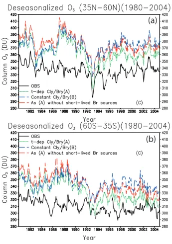
3.3 Mid-latitude column ozone

Figure3shows a comparison of zonal mean column O₃in the NH and SH mid latitudes from satellite observations and the model runs. The observations are the merged TOMS/SBUV dataset of R. Stolarski (personal communication, 2005). This dataset

20

uses Nimbus 7 TOMS and SBUV, the NOAA 9, 11, and 14 SBUV/2 and the Earth Probe TOMS. Generally the model columns overestimate the observations. This difference is largest in the late 1980s when the model values in the NH are up to 70 DU too large. Compared with previous full chemistry SLIMCAT runs this worse agreement is due to the extension of the model lower boundary from around 350 K down to the surface. The

25

model now predicts O₃in the lowermost stratosphere and with the ERA40 analyses this is overestimated, similar to the polar regions (see Sect. 3.2).

(10)

ACPD

Full Screen / Esc

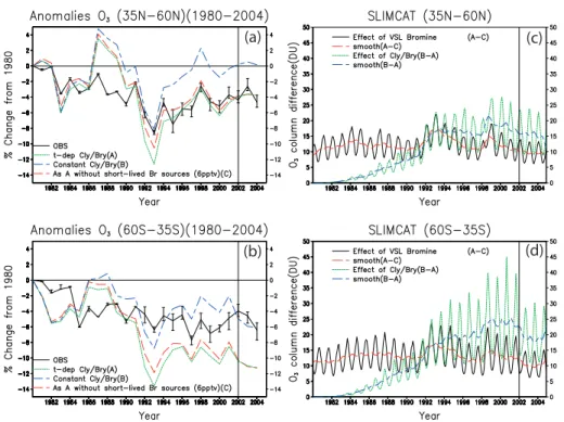
EGU (expressed as % change since 1980) for the NH (35◦N–60◦N) and the SH (35◦S–

60◦S). Overall, model run A reproduces the observed decrease in column ozone in these regions between 1980 and the mid 1990s, although it overestimates the de-crease in the SH. As seen in previous CTM runs (e.g. Chipperfield, 2003) the model does capture some of the long-term variability although there are significant di

ffer-5

ences. The model has a strong positive deviation in the late 1980s and too strong a dip in the early 1990s. These are likely more accentuated in our run than that of Hadjini-colaou et al. (2005) because we include the full depth of the stratosphere. In addition some of the observed variability on the timescale of a few years is reproduced by the model, especially before the early 1990s. Later in the 1990s the modelled variations

10

do not agree as well and this again is likely related at least in part to the changing ECMWF analyses. It should be noted that after the change of the model forcing winds from ERA-40 to operational winds (31 December 2001) there is a significant change in the modelled anomaly in the SH.

Including the additional constant 5 pptv of Br_y from short-lived species tends to

de-15

crease mid-latitude column O₃ by around 10 DU throughout the model runs (Figs.4c, d). When the O₃ anomaly is calculated with respect to the appropriate 1980 levels, the anomaly from run C is very similar to run B except during periods of high aerosol loading where an enhanced decreased (of around 2%) is seen.

3.4 Lower and upper stratosphere

20

Figure 5 shows the variation in O₃ mixing ratio at NH and SH mid-latitudes at 20 km and 40 km for 3 model runs. In the upper stratosphere there is some variability but O₃ declines from the late 1980s through 2004. The decline is larger in the runs with increasing halogens but run B still shows a similar variation. In the lower stratosphere the O₃variation is clearly more reflective of what happens to the total column with

mini-25

mum values around 1993 followed by some increase. Note, however, that in the SH the column decrease after the change of forcing analyses in 2002, is not seen in the 20 km O₃ but does coincide with an abrupt decrease at 40 km. Figure 6 shows the

(11)

equiv-ACPD

Full Screen / Esc

EGU alent results for the modelled total inorganic chlorine (Cl_y). This shows the expected

increase through the late 1990s followed by a peak and the recent turnover. In the model this seems to have occurred in 1998–2000 at 40 km (run A); in the lower strato-sphere the dynamical variability makes the situation less clear, through the maximum modelled values occurred around 2001. Given this change in Cl_y, which we expect to

5

be a main driver for the model chemical O₃trend, it is useful to explore the factors that have contributed to the modelled O₃variations in the upper and lower stratosphere.

In the upper stratosphere, which is chemically more simple, the model O₃continues to decline through 2004 despite the turnover in model Cl_y. Figures7,8and9show the corresponding plots of CH₄, ClO and temperature. Over this time period the changes in

10

stratospheric CH₄are first driven by the increase in tropospheric CH₄. In addition there is interannual variability in atmospheric transport which causes variability in CH₄, which is generally anticorrelated with Cl_y due to the opposing gradients. Notably, between 1996 and 2001 at 20 km in the NH CH₄decreased, indicating a large role for dynamics in the model here. In the upper stratosphere there is larger relative variability.

15

Figures8a, b shows the variation of ClO at 40 km. Changes in CH₄ will affect the partitioning of the two main Cl_y reservoirs ClO and HCl; increases in CH₄ will tend to decrease ClO. Therefore the modelled CH₄ changes after 2000, when Cl_y is decreas-ing, have tended to increase NH ClO (i.e. oppose Cl_y changes) and decrease SH ClO. This leads to an overall larger decrease in ClO in the SH.

20

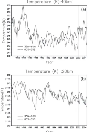
Finally, Figs.9a, b shows the model (ECMWF) temperatures at 40 km. In the upper stratosphere warmer temperatures tend to decrease O₃due to faster catalytic loss. In the early 1980s the analyses show unrealistically large T variations of around 10 K in 2 years. The large decrease of temperature from 1984 to 1986 in both hemispheres leads to the O₃ increase seen in Figs. 5a, b. After 1986 the NH temperatures tend

25

to increase while the SH temperatures remain fairly constant with an abrupt increase around 2002. Therefore, in the model, upper stratosphere O₃ does not increase post 2000, despite decreasing Cl_y, due to (i) decreasing CH₄and increasing temperatures in the NH and (ii) abrupt changes in the model meteorological fields in early 2002

(12)

ACPD

Full Screen / Esc

EGU in the SH due to a change of forcing analyses. This again illustrates the problem of

diagnosing long-term changes from a single CTM experiment. Clearly, direct diagnosis of O₃ recovery from the effects of halogen changes can be achieved by taking the difference between appropriate chemical model experiments.

3.5 Mid-latitude profile changes

5

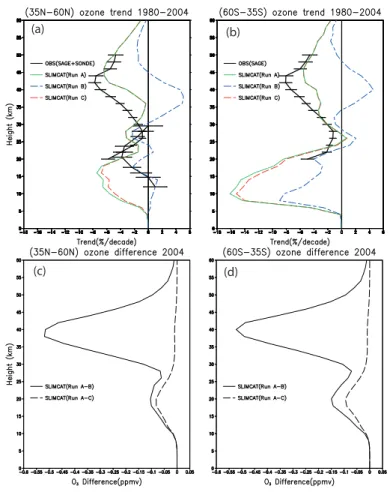
An important step in the attribution of ozone changes to the correct cause is the match-ing of “fmatch-ingerprints” between observed and modelled changes (e.g. WMO, 2003). One such important test is to examine the profile of modelled ozone changes which con-tributes to the column mid-latitude changes described above. Figure 10 shows es-timates of the modelled trend for 1980–2004 for runs A, B and C, along with di

ffer-10

ences between model runs for the year 2004 which shows the effect of increasing halogens (A–B) and additional bromine (A–C). The trends were diagnosed using a model (Ziemke et al., 1997) with a regression onto a term for the Effective Equivalent Stratospheric Chlorine (EESC). The trend was converted from units of O₃loss per unit EESC to %/decade by using the near-linear rate of change of EESC with time in the

15

1980s.

The observed trend, based on sonde data in the lower stratosphere and satellite data higher up, shows a characteristic double peak structure with maximum trends of around −9%/decade near 40 km and -6%/decade in the NH lower stratosphere. (There is not enough sonde date in the SH for a trend analysis). The basic model run A tends

20

to capture this structure although the 40 km peak is smaller and displaced upwards slightly while in the NH lower stratosphere the modelled trend is much larger than ob-served below 15 km. The modelled lower stratosphere (LS) trend is larger in the SH, although there is no data for comparison. The trend from model run B differs from zero and also shows some of the vertical structure seen in the trend from run A. In particular,

25

it is interesting to note that run B has a positive trend near 40 km and a large nega-tive trend in the SH lower stratosphere. Hence, this component of the modelled trend (i.e. dynamically induced or due to other chemistry) has acted to offset the halogen

(13)

ACPD

Full Screen / Esc

EGU trend in the upper stratosphere (US) and increased the trend in the SH lower

strato-sphere. Figures10c, d show the difference in O₃between selected runs. These profiles are much smoother and show the effect in 2004 of the overall halogen increases and increased stratospheric Br_y. The LS changes are now more symmetrical between the NH and SH. The 40 km change of −0.5 ppmv (Fig. 10) corresponds to a change of

5

around −7%/decade for the 1985–2000 change in Cl_y. The lower stratospheric change of −0.15 ppmv corresponds to around −5 to −7%/decade over the same period.

Clearly, taking the difference between 2 model runs with the same meteorology gives a much more direct and cleaner signal of the relevant chemical forcing. This is also seen in Fig.11which shows a latitude height plot of the percentage difference between

10

runs A and B. The increasing halogens (runs A–B) gives the characteristic double peak structure with loss near 40 km due to the ClO+O cycle as well as loss in the lower stratosphere near 20 km. The “cleaner” diagnosis of ozone changes seen in Figs.10c, d and11 tend to be more similar to the trends derived from observations in terms of spatial variations (e.g. Fig. 4.9 of WMO, 2003). The equivalent plot of Fig.11diagnosed

15

from the trend of run A is alot noisier (not shown), but the differences can already be seen in Fig.10a ,b for mid-latitudes. Again, it seems that the meteorological analyses used to force the model introduce spurious variations which affect the trend calculation, while diagnosis of trends in the real atmosphere might separate a cleaner ’chemical’ signal.

20

Finally, from Fig.10we can note that the effect of increased bromine is confined to the lower stratosphere where the bromine cycles are important.

4 Conclusions

We have used the SLIMCAT off-line 3-D chemical transport model to investigate long-term changes in stratospheric ozone in the mid-latitude lower and upper stratosphere.

25

The CTM was forced using ECMWF ERA-40 reanalyses from 1977 until the end of 2001 and then operational analyses until the end of 2004.

(14)

ACPD

Full Screen / Esc

EGU A key message from these simulations is that care is needed when using analysed

meteorological data, or results which depend on such data, for long-term trend studies. Models which are forced by reanalyses certainly capture much of the apparent interan-nual variability (e.g. in column ozone) but the analyses also exhibit spurious features. For the ERA-40 data used here these include producing very large NH CTM ozone

5

columns in the late 1980s and upper stratospheric temperature decreases around 1985 which lead to local ozone increases. Nevertheless, the analyses do provide realis-tic meteorology (e.g. more realisrealis-tic polar temperatures than would be calculated by a GCM) against which chemical experiments can be performed.

A number of CTM experiments have been performed to assess the impact of

increas-10

ing halogens and bromine from short-lived species on mid-latitude ozone. The basic model reproduces the observed anomalies of column ozone in the NH, with the excep-tion of the late 1980s, where the model has too large values, and an overestimate of the dip around 1992. The model generally performs less well for the SH column ozone anomaly relative to 1980 values. The model overestimates the decrease through 2002,

15

although this could be explained by an overestimation of the 1980 values, and also pro-duces a marked decrease around 1993 which is not observed. This feature is seen in essentially all 2-D and 3-D model runs and its absence in the observations has not been explained (see WMO, 2003).

Trends in the model runs have been analysed using a regression model and by

20

fitting the chemical signal to an EESC function. The modelled trend profile captures the observed double peak structure with large losses in the lower stratosphere and the upper stratosphere, although the model appears to overestimate the trends in the very low stratosphere near 10 km. However, the trends from the basic model do not show such a clean structure as the observations. Model-model differences which isolate

25

the effect of increasing halogens show a “fingerprint” which matches the observations much better, especially for the variation with latitude and height. We would argue that the trend calculation is somewhat compromised by unrealistic variations in the analyses used to force the model.

(15)

ACPD

Full Screen / Esc

EGU Finally, the model has been used to investigate the variation of O₃ at 40 km. In this

region the model O₃ is affected by variations in temperature and transport of CH₄. Together these produce variations which can be larger than those due to changes in Cl_y loading. Although the modelled variations in temperature and long-lived tracers may not be realistic, this demonstrates the difficulty in separating such effects from

5

ozone observations in the real atmosphere. This emphasises that the diagnosis of the onset of recovery from halogen-catalysed loss at 40 km, similar to that which has been performed in the Antarctic LS (Yang et al., 2005), needs careful separation of these effects.

Acknowledgements. This work was supported by the UK Natural Environment Research Coun-10

cil and by the EU through the SCOUT-O3 project. We thank V. Fioletov for help with the trend analysis. We thank BADC for helping to provide the ECMWF analyses.

References

Chipperfield, M. P.: Multiannual simulations with a three-dimensional chemical transport model, J. Geophys. Res., 104, 1781–1805, 1999.

15

Chipperfield, M. P.: A three-dimensional model study of long-term mid-high latitude lower strato-sphere ozone changes, Atmos. Chem. Phys., 3, 1253–1265, 2003.

Chipperfield, M. P.: A new version of the TOMCAT/SLIMCAT off-line chemical transport model: Intercomparison of stratospheric tracer experiments, Q. J. Roy. Meteorol. Soc., in press, 2006.

20

Chipperfield, M. P. and Jones, R. L.: Relative influences of atmospheric chemistry and transport on Arctic O₃trends, Nature, 400, 551–554, 1999.

Chipperfield, M. P., Feng, W., and Rex, M.: Arctic Ozone Loss and Climate Sensitiv-ity: Updated Three-Dimensional Model Study, Geophys. Res. Lett., 32(11), L11813, doi:10.1029/2005GL022674, 2005.

25

Dorf, M.: PhD thesis, University of Heidelberg, Heidelberg, Germany, 2005.

Dorf, M., B ¨osch, H., Butz, A., Camy-Peyret, C., Chipperfield, M. P., Engel, A., Goutail, F., Grunow, K., Hendrick, F., Hrechanyy, S., Naujokat, B., Pommereau, J.-P., Van Roozendael, M., Sioris, C., Stroh, F., Weidner, F., and Pfeilsticker, K.: Balloon-borne stratospheric BrO

(16)

ACPD

Full Screen / Esc

EGU

measurements: Comparison with Envisat/SCIAMACHY BrO limb profiles, Atmos. Chem. Phys. Discuss., 5, 13 011–13 052, 2005.

Feng, W., Chipperfield, M. P., Davies, S., Sen, B., Toon, G., Blavier, J. F., Webster, C. R., Volk, C.M., Ulanovsky, A., Ravegnani, F., von der Gathen, P., Jost, H., Richard, E. C., and Claude, H.: Three-dimensional model study of the Arctic ozone loss in 2002/2003 and comparison

5

with 1999/2000 and 2003/4, Atmos. Chem. Phys., 5, 139–152, 2005.

Hadjinicolaou, P., Jrrar, A., Pyle, J. A., and Bishop, L.: The dynamically driven long-term trend in stratospheric ozone over northern mid-latitudes, Q. J. Roy. Met. Soc., 128, 1393–1412, 2002.

Hadjinicolaou, P., Pyle, J. A., and Harris, N. R. P.: The recent turnaround in stratospheric ozone

10

over northern middle latitudes: A dynamical modelling perspective, Geophys. Res. Lett., 32, L12821, doi:10.1029/2005GL022476, 2005.

Montzka, S., Butler, J., Hall, B., Mondell, D., and Elkins, J.: A decline in tropospheric organic bromine, Geophys. Res. Lett., 30, 1826–1829, 2003.

Newman, P. A., Gleason, J. F., McPeters, R. D., and Stolarksi, R. S.: Anomalously low ozone

15

over the Arctic, Geophys. Res. Lett., 24, 2689–2692, 1997.

Pfeilsticker K., Sturges, W. T., B ¨osch, H., Camy-Peyret, C., Chipperfield, M. P., Engel, A., Fitzen-berger, R., M ¨uller, M., Payan, S., and Sinnhuber, B.-M.: Lower stratospheric organic and inorganic bromine budget for the Arctic winter 1998/99, Geophys. Res. Lett., 27, 3305–3308, 2000.

20

Salawitch, R. J., Weisenstein, D. K., Kovalenko, L. J., Sioris, C. E., Wennberg, P. O., Chance, K., Ko, M. K. W., and McLinden, C. A.: Sensitivity of ozone to bromine in the lower stratosphere, Geophys. Res. Lett., 32, L05811, doi:10.1029/2004GL022226, 2005.

Sinnhuber, B.-M., Arlander, D. W., Bovensman, H., Burrows, J. P., et al.: Comparison of mea-surements and model calculations of stratospheric bromine monoxide, J. Geophys. Res.,

25

107, 4398, doi:10.1029/2001JD000940, 2002.

Stolarski, R. S., Douglass, A. R., Steenrod, S., and Pawson, S.: Trends in stratospheric ozone: Lessons learned from a 3D chemical transport model, J. Atmos. Sci., in press, 2006. Uppala, S. M., Kallberg, P. W., Simmons, A. J., Andrae, U., et al.: The ERA-40 Re-analysis, Q.

J. Roy. Meteorol. Soc., 131, 2961–3012, doi:10.1256/qj.04.176, 2005.

30

World Meteorological Organization (WMO): Scientific Understanding of Ozone Depletion: 2002, Global Ozone Research and Monitoring Project – Report No. 47, World Meteorological Or-ganization, Geneva, 2003.

(17)

ACPD

Full Screen / Esc

EGU

Yang, E. S., Cunnold, D. M., Newchurch, M. J., and Salawitch, R. J.: Change in ozone trends at southern high latitudes, Geophys. Res. Lett., 32, L12812, doi:10.1029/2004GL022296, 2005 Ziemke, J. R., Chandra, S., McPeters, R. D., and Newman, P. A.: Dynamical proxies of column

ozone with applications to global trend models, J. Geophys. Res., 102, 6117–6129, 1997.

(18)

ACPD

Full Screen / Esc

EGU Table 1. CTM experiments

Run Halogens Br_ysources

A time-dependent CH₃Br+ Halons + VSLS + trop. Bry

B fixeda CH₃Br+ Halons + VSLS + trop. Bry

C time-dependent CH₃Br only

D time-dependent CH₃Br only but total bromine scaled to match A

a

(19)

ACPD

Full Screen / Esc

EGU Fig. 1. DOAS-observed profile of BrO volume mixing ratio (pptv, circles) at Kiruna (67◦N) on

24 March 2004. Also shown are model profiles of Br_yspecies and bromine source gases from runs A (solid lines) and D (dashed lines).

(20)

ACPD

Full Screen / Esc

EGU Fig. 2. Mean TOMS column O₃poleward of (top) 63◦N in March and (bottom) 63◦S in October

(updated from Newman et al., 1997). Also shown are the corresponding model (chemically integrated and passive ozone) results from runs A and B. (The passive O₃tracer is reset equal to the chemically integrated O₃every 1 July and 1 January then advected in the model without any further chemical change. The difference between the passive O3 and the corresponding

chemically integrated O3indicates the chemical O3loss since this time). Note different ranges

(21)

ACPD

EGU Fig. 11. Latitude-height plot of the percentage difference in zonal mean annual mean ozone