HAL Id: hal-00299513
https://hal.archives-ouvertes.fr/hal-00299513
Submitted on 15 Apr 2008
HAL is a multi-disciplinary open access
archive for the deposit and dissemination of
sci-entific research documents, whether they are
pub-lished or not. The documents may come from
teaching and research institutions in France or
abroad, or from public or private research centers.
L’archive ouverte pluridisciplinaire HAL, est
destinée au dépôt et à la diffusion de documents
scientifiques de niveau recherche, publiés ou non,
émanant des établissements d’enseignement et de
recherche français ou étrangers, des laboratoires
publics ou privés.
monitoring ultra low frequency activity in California
J. Cutler, J. Bortnik, C. Dunson, J. Doering, T. Bleier
To cite this version:
J. Cutler, J. Bortnik, C. Dunson, J. Doering, T. Bleier. CalMagNet ? an array of search coil
magne-tometers monitoring ultra low frequency activity in California. Natural Hazards and Earth System
Science, Copernicus Publications on behalf of the European Geosciences Union, 2008, 8 (2),
pp.359-368. �hal-00299513�
Nat. Hazards Earth Syst. Sci., 8, 359–368, 2008 www.nat-hazards-earth-syst-sci.net/8/359/2008/ © Author(s) 2008. This work is licensed under a Creative Commons License.
Natural Hazards
and Earth
System Sciences
CalMagNet – an array of search coil magnetometers monitoring
ultra low frequency activity in California
J. Cutler1,2, J. Bortnik3,2, C. Dunson2, J. Doering2, and T. Bleier2
1Space and Systems Development Laboratory, Department of Aeronautics and Astronautics, 496 Lomita Mall, Stanford
University, Stanford, California, USA
3Department of Atmospheric and Oceanic Sciences, Room 7115, Math Sciences Building, UC Los Angeles, California,
90095–1565, USA
2Quakefinder, LLC, 250 Cambridge Avenue, Palo Alto, California, 94306, USA
Received: 19 September 2007 – Revised: 6 December 2007 – Accepted: 6 December 2007 – Published: 15 April 2008
Abstract. The California Magnetometer Network (CalMag-Net) consists of sixty-eight triaxial search-coil magnetome-ter systems measuring Ultra Low Frequency (ULF), 0.001– 16 Hz, magnetic field fluctuations in California. CalMagNet provides data for comprehensive multi-point measurements of specific events in the Pc 1–Pc 5 range at mid-latitudes as well as a systematic, long-term study of ULF signals in ac-tive fault regions in California. Typical events include ge-omagnetic micropulsations and spectral resonant structures associated with the ionospheric Alfv´en resonator. This paper provides a technical overview of the CalMagNet sensors and data processing systems. The network is composed of ten reference stations and fifty-eight local monitoring stations. The primary instruments at each site are three orthogonal in-duction coil magnetometers. A geophone monitors local site vibration. The systems are designed for future sensor ex-pansion and include resources for monitoring four additional channels. Data is currently sampled at 32 samples per second with a 24-bit converter and time tagged with a GPS-based timing system. Several examples of representative magnetic fluctuations and signals as measured by the array are given.
1 Introduction
A number of magnetometer networks are deployed through-out the world to measure magnetic field variations to provide insight into the two-dimensional geographic distribution and dynamic variation of current flow and particle precipitation in the magnetospheric-ionospheric system.
Correspondence to: J. W. Cutler
(jwc@stanford.edu)
For example, the CANOPUS array deployed in north-ern Canada contains thirteen fluxgate magnetometers (along with additional riometers, photometers, and imaging sys-tems) to monitor high-latitude ionospheric currents and au-roral activity (Rostoker et al., 1995). The CANOPUS array is currently being expanded to include an additional 15 triax-ial fluxgate magnetometers and eight two-axis induction coil magnetometers (Mann et al., 2004).
Another example, the Finnish pulsation magnetometer chain (Hebden et al., 2005), monitors geomagnetic pulsa-tions with seven induction coil systems in Finland and one in Crete.
Magnetometer arrays are also used to probe conductiv-ity structures of the Earth. Geomagnetic depth sounding (GDS) techniques use triaxial magnetic measurements to ob-tain orientations to nearby conductivity anomalies (Gregori and Lanzerotti, 1980; Schmucker, 1985). Typical GDS mea-surement examples include the survey of northern Italy by Armadillo et al. (2001) and a survey of North America by Neal et al. (2000).
Complementing the GDS technique which relies solely on magnetic field measurements, are magnetotelluric methods which use three axis magnetic and two axis electric measure-ments to determine the depth-profile of conductivity struc-tures (Simpson and Bahr, 2005).
For example, a magnetotelluric network has been de-ployed as part of the Parkfield earthquake prediction experi-ment (Bakun and Lindh, 1985; Roeloffs and Langbein, 1994) to monitor sections of the San Andreas fault in California. UC-Berkeley has deployed two sites (Morrison et al., 1996), and an additional three sites are under development by Stan-ford University for deployment in the San Francisco Bay Area (Bijoor et al., 2005).
235˚ 235˚ 240˚ 240˚ 245˚ 245˚ 35˚ 35˚ 40˚ 40˚ HLD PTV MET LEB JLN YUC CRN EMP HDW OCT California Nevada Legend QF−HS QF−1000/1003 QF−1005
Fig. 1. A map of sensor locations in CalMagNet. The QF-1005
reference stations are shown as yellow triangles and labeled with station codes. Light blue and red triangles represent HS and QF-1000/1003 stations respectively. Station locations coarsely reflect the San Andreas and adjacent fault systems, and are placed in high probability earthquake regions.
To provide additional low-latitude magnetic field measure-ments, we have developed and deployed the California Mag-netometer Network (CalMagNet), an array of sixty-eight in-duction coil magnetometer systems.
L-shell values, which approximately represent the number of Earth radii that the local magnetic field line extends into space (Campbell, 2003), of the CalMagNet sensor systems range from 1.6–1.9.
Example signals include geomagnetic micropulsations (Jacobs, 1970; Bortnik et al., 2007) and spectral resonant structures (SRS) associated with the ionospheric Alfv´en res-onator (Belyaev et al., 1990).
CalMagNet is also monitoring ULF activity in active fault regions of California. Reports have appeared in the litera-ture indicating anomalous electromagnetic activity preced-ing large quakes (e.g. see reviews by Hayakawa (1999), Park et al. (1993), Johnston (1997) and the references therein).
In direct relevance to this paper, we note two observations made during large recent California earthquakes.
Fraser-Smith et al. (1990) and Bernardi et al. (1991) describe an anomalous signal preceding the the 18 Octo-ber 1989 M 7.1 earthquake that occurred in Loma Prieta, California. However, Park et al. (2007) detected no
anoma-lous activity with electric dipoles preceeding the M 6.0 earth-quake at Parkfied, California, on 28 September 2004.
Therefore, CalMagNet is being used for a systematic sur-vey of ULF activity in diverse fault regions to assess any po-tential correlations between various earthquake events and ULF signals.
In this paper, we describe the CalMagNet sensor systems. In Sect. 2, we describe our network topology and strategy for sensor placement.
In Sect. 3, details of the sensor systems are given, includ-ing a system block diagram, analog to digital conversion pa-rameters, and sensor transfer function and noise floors.
In Sect. 4, we give examples of measured ULF signals and events.
We conclude in Sect. 5 with a summary of system capabil-ities and data distribution methods.
2 Network topology
Site selection for CalMagNet sensors is primarily directed by our long-term strategic goal to provide sensitive mea-surements of magnetic field fluctuations in the ULF range, located as close as possible to all land-based earthquakes greater than magnitude 5 in California. With a desired maxi-mum distance of 10 km from an epicenter, this would require over 100 sensor systems along the over 2000 km of active fault zones in California. Due to cost constraints, this is not currently feasible.
Therefore, we guide our network topology and sensor placement with statistical methods indicating potentially higher probability locations for large earthquakes. Areas of increased seismic potential are identified from the out-put of a technique for describing driven, nonlinear threshold systems, the Phase Dynamics Probability Change (PDPC) method (Tiampo et al., 2002). We place our sensors in these “hotspots” to potentially improve the likelihood of proximal measurements of a large earthquake.
We have deployed four classes of sensor systems, the QF-1005, QF-1003, QF-1000, and QF-HS, to extend the range of measurement opportunities. Design details are given in the next section. Ten, high-performance systems, the QF-1005 s, perform detailed measurements of ULF magnetic ac-tivity. Positions of these ten systems are given in Table 1. The remaining fifty-eight sensor systems are lower cost sys-tems that extend the geographic coverage of the network to increase our likelihood of measurements near a large earth-quake, but with reduced measurement sensitivity at lower frequencies. Figure 1 shows the location of CalMagNet sen-sor systems.
Complementing the installed sites, we have a transportable QF-1005 for specialized field campaigns of short-term mea-surements (weeks to months). Similar in operational prin-ciple to the system described by Karakelian et al. (2000), this transportable unit will be installed near the epicenter of
J. W. Cutler et al.: CalMagNet – A ULF Magnetometer Network in California 361
Table 1. Location summary of the ten QF-1005 sensor systems in geodetic coordinates with calculated L-shell values.
ID Name Lat. (◦N) Lon. (◦W) Elev. (m) L-Value HDW Honeydew 40.244 124.116 123 1.982
HLD Healdsburg 38.694 122.947 85 1.895 EMP East Milpitas 37.415 121.780 637 1.832 PTV Portola Valley 37.336 122.196 457 1.822 MET Mettler 35.055 119.031 136 1.731 BEC LeBec 34.827 118.897 1324 1.721 YUC Yucaipa 34.072 117.081 981 1.701 CRN Corona 33.834 117.585 379 1.684 OCT Ocotillo Wells 33.142 116.136 60 1.665 JLN Julian 33.101 116.597 1280 1.658
Table 2. Summary of CalMagNet sensor system characteristics. System Type
Characteristic
HS 1000 1003 1005
Number of stations 24 11 23 10
Geophone no no yes yes
Extra Channels 0 0 4 4
Samples per second 20 20 20 32
Bits per sample 12 12 16 24
GPS Timing no no yes yes
Coil Specs.
Gain @ 1 Hz (V/pT) 2×10⁻³ 2×10⁻³ 2×10⁻³ 10−3
Noise @ 1 Hz (pT) 3 3 3 0.1
Pass Band (Hz) 0.5–4 0.5–4 0.5–4 0.001–12
future earthquakes to search for any post-earthquake ULF
anomalies. It will also be used for specialized remote
referencing measurements when local signals under study are dominated by larger, wide-area signals (Egbert, 1997; Larsen, 1989).
3 Sensor systems
CalMagNet is composed of four classes of sensor systems. Their characteristics are summarized in Table 2, including the number and types of systems, induction coil parameters, extra channels, sampling rate and resolution, and GPS time-tagging. In the rest of this section, we provide a detailed sum-mary of the ten high-performance stations, the QF-1005 s, and include brief summaries of the additional three classes.
3.1 QF-1005 System
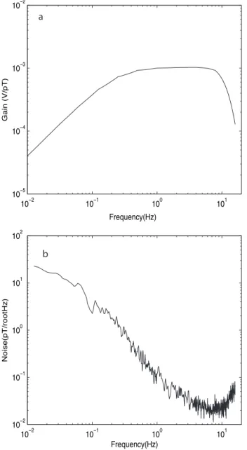
Figure 2 is a block diagram of the major components of the QF-1005. The primary instruments for the QF-1005 are three orthogonal induction coil magnetometers, the ANT/4, designed and manufactured by Zonge Engineering (Zonge, 2006). The transfer function and noise floor and gain of a typical ANT/4 coil are plotted in Fig. 3, panels a and b, re-spectively and summarized in Table 3.
A high pass analog filter rolls off the gain below 0.25 Hz to suppress the monotonic increase in signal strength at lower frequencies. An anti-aliasing, analog filter rolls off the gain above 12 Hz to suppress 60 Hz noise while still allowing de-tection of the first Schumann resonance. During calibra-tion, coil characteristics are optimized to achieve high co-herence between separate coils, greater than 99%. After field measurements during system testing, an additional filter was installed to further reduce 60 Hz noise contamination. An analog, 5-pole Butterworth filter with a 11.5 Hz cutoff fre-quency was installed to provide a total of 100 dB attenuation at 60 Hz.
Three coils are installed at each site. The first coil is aligned in the geodetic north/south direction (15◦±2◦ west
of geomagnetic north) with positive signal levels indicating a magnetic field vector pointing to the north.
The second coil is aligned in the geodetic east/west direc-tion (15◦±2◦south of geomagnetic east) with positive signal levels indicating a magnetic field vector pointing to the east. The third coil is installed vertically using a plumb line. A positive signal indicates a magnetic field vector pointing in the down direction.
A calibration signal is applied twice a day to each coil. At approximately local noon and midnight (within 5 min of the hour mark), an 8 nT peak-to-peak signal at 1 Hz is applied to each coil through a calibration coil built into the magnetome-ters. The calibration signal lasts five minutes. The sensor response is monitored for any degradation in signal quality.
Analog data channels are digitized by a commercial 8-channel, 24-bit analog-to-digital converter system, the PAR 8 CH by Symmetric Research. Samples are taken at a frequency of 32 samples per second. The sample rate is adjustable and was set to provide reasonable data file sizes for our frequency band of interest, less than 10 Hz. It was also set such that any 60 Hz signal contamination would fold over onto 4 Hz during Fourier-based spectral analysis (ver-sus 0 Hz when sampled at 30 Hz). The PAR 8 CH uses eight independent analog-to-digital converter chips, the ADS 1210 from Burr Brown, to reduce cross-talk noise contamination.
text text Junction Box 2 m 2 m 2 m Hx--channel 2 (Zonge Ant-4) Geophone textAir Conductivity Sensor Analog Filter 24 bit Digitizer 8-channels GPS Garmin GPS-16HVS CPU 40GB Hard drive Power System Batteries
LED Status Lights WiFi Transceiver WiFi Transceiver Satellite-Based Internet Geophone--channel 4 (Giscogeo SN4-4.5) Air Cond.--channel 5 (Quakefinder experimental) ~ 15 m ~ 5 m ~ 1 m 3 expansion channels 10-1 00 m AC Outlet Pre Amp Pre Amp Hz--channel 3 (Zonge Ant-4) Hy--channel 1 (Zonge Ant-4) Pre Amp
Fig. 2. Block diagram of QF-1005 system. Hx, Hy. and Hz represent the 3 search-coil magnetometers, oriented in the North, East and nadir
directions respectively. A single axis geophone measures local motion. An experimental air conductivity sensor is attached, and there are three spare channels for future sensor expansions. The large gray central box houses analog filters, sampling systems, a computer, power systems, and communication equipment. Data transfers to the data center typically occur over satellite phone or Internet connections.
The primary CalMagNet instruments, namely the induc-tion coil magnetometers, are susceptible to moinduc-tion-induced noise. Oscillating microradian tilts of the induction coils in the ambient earth magnetic field result in signals that are sim-ilar to naturally occurring signals. Ideally, coils should be placed near broadband seismometer stations to provide de-tailed monitoring of ground motion (Karakelian et al., 2000). Due to cost constraints, CalMagNet systems are not all lo-cated near broadband seismometer stations. To augment the existing wide-area seismic monitoring stations, we have in-stalled secondary sensors on the systems, a Giscogeo geo-phone SN 4–4.5, that are five times more sensitive than the induction coils to motion at frequencies greater than 4 Hz.
Four of the eight channels of the data acquisition are avail-able for experimental and future sensor expansion. Currently, at several sites, experimental air conductivity sensors are in-stalled. A number of experimental dipole electric antennas
from Quasar Federal Systems (Delory et al., 2005) will be deployed in the near future to test their operation.
Each system is controlled by an embedded PC-104 proces-sor system that manages data acquisition and transfer. Raw sample data from the sensors is stored in five minute blocks, and archived locally on a standard 2.5 inch hard drive with a capacity greater than 40 GB. This provides over 600 days of storage of 8 channels sampled at 32 Hz and 24 bits for local archiving during the presence of communication failures.
Raw data collected over a 24 h period is transferred nightly to a data center over commercial, satellite-based Internet links. The data center archives sensor data, monitors health of sensor systems, and produces a variety of products such as daily dynamic spectrograms (Cutler, 2005). Future upgrades will stream the data in near real-time to the data center for more timely processing.
J. W. Cutler et al.: CalMagNet – A ULF Magnetometer Network in California 363 10−2 10−1 100 101 10−5 10−4 10−3 10−2 G a in (V/ p T ) 10−2 10−1 100 101 10−2 10−1 100 101 102 N o ise (p T /ro o tH z) Frequency(Hz) a b Frequency(Hz)
Fig. 3. Characteristics of a single ANT/4 magnetometer. (a) Plot
of gain versus frequency for the ANT/4, pre-amplifier, and filter.
(b) Noise floor of the ANT/4 magnetometer. These are measured
values from coils deployed in CalMagNet. They were obtained by taking two coils to a remote, low-noise location, and differencing the signals to remove common mode signal while leaving only the internal noise of the system. Values differ slightly from Table 3 due to local environmental noise conditions during this particular test.
GPS-based time tagging of data samples is provided by a Garmin GPS–16 HVS receiver. The pulse per second output of the receiver (accurate to ±1 microsecond) is combined with a 800 nanosecond counter on the PAR 8 CH to provide an overall timing error less than 3.3 microseconds.
Table 3. Summary of typical Zonge ANT/4 magnetometer gain and
noise characteristics. Values are average measurements made from multiple ANT/4 tests in quiet locations.
Frequency (Hz) Gain (V/pT) Noise (pT/Hz12)
0.001 3 x10⁻⁶ 250 0.01 3 x10⁻⁵ 15
0.1 3 x10⁻⁴ 1.5
1 10−3 0.1
10 10−3 0.02
3.2 Additional sensor systems
In 1998, the initial CalMagNet sites, QF-HS systems, were deployed through an educational program where high school students built low-cost, “Heathkit-like” systems. The educational program taught students about scientific instru-mentation and geomagnetic studies.
In 2001, we began upgrading to commercial versions, in-creasing both reliability and sensitivity. These are the QF-1000 systems. In 2003, NASA provided funding to build and deploy twenty new sensors in the Mojave Desert of southern California. Through this NASA contract, our upgraded sen-sor system, the QF-1003, now includes GPS time synchro-nization, a Globalstar communication system, an air conduc-tivity sensor, and a geophone. The third generation system, the QF-1005, has been described above.
4 Example signals and analysis
Survey and classification of ULF signal sources received by the CalMagNet is underway in our data center (Cutler, 2005). Typical signals include geomagnetic pulsations re-sulting from ionospheric and magnetospheric processes (Ja-cobs, 1970), cultural noise such as public transportation sys-tems (Liu, 1999), and movement of the coil in the earth’s magnetic field (Karakelian et al., 2000). In this section, we provide an overview of typical signals received by CalMag-Net and example analysis efforts.
4.1 Geomagnetic pulsations
Pc 1 geomagnetic pulsations are typical signals received by the network (Jacobs, 1970).
These waves are thought to originate in the equatorial re-gion of the outer magnetosphere (Cornwall, 1965), propagate along field lines into the high latitude ionosphere, and propa-gate down to low latitudes within the F 2-region ionospheric duct (Fraser, 1968; Manchester, 1968), where they are ob-served by our instruments.
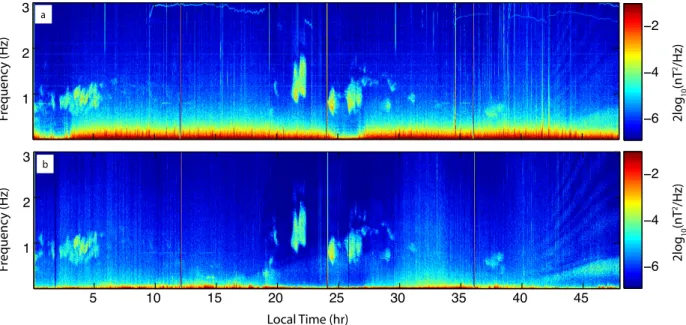
Figure 4 shows Pc 1 geomagnetic micropulsations
re-ceived by the network. Data from 17–18 April 2006 is
plotted from two sites, East Milpitas near San Francisco and
1 2 3 −6 −4 −2 5 10 15 20 25 30 35 40 45 1 2 3 Local Time (hr) −6 −4 −2 Fr equenc y (Hz) Fr equenc y (Hz) 2lo g10 (nT 2/Hz) 2lo g10 (nT 2/Hz) a b
Fig. 4. Dynamic spectrograms on 17–18 April 2006 at two CalMagNet Sites: (a) East Milpitas (EMP), near San Francisco, and (b) Julian
(JLN), near San Diego. Strong Pc 1 pulsations occur at both sites between 0.5 and 2 Hz periode.
Julian near San Diego. Multiple Pc1 pulsations are seen dur-ing the early morndur-ing and night at both sites due to a strong magnetic storm that occurred 14 April 2006.
4.2 Ionospheric Alfv´en Resonator
Another common ULF signal is the spectral resonant struc-ture (SRS) of the the ionospheric Alfv´en resonator (IAR) (Bosinger et al., 2002). According to current models, the primary excitation source is electromagnetic emissions from global thunderstorm activity (Belyaev et al., 1990). Charac-teristics of the IAR such as the fundamental frequency are governed by local ionospheric conditions. Distributed mea-surements by CalMagNet of SRS properties allow measure-ment of ionospheric properties over California.
Wave parameters of typical SRS activity as measured by
CalMagNet are shown in Fig. 5. These parameters are
calculated following the methodology of Means (1972) and Fowler et al. (1967) using the wave detection and characteri-zation approach outlined by Bortnik et al. (2007).
Plot a shows the zenith angle of three days of data from site JLN starting from noon local time on 03 May 2006. Plots b–f plot additional wave parameters from a focused time period, 21 h of data starting at 1400 local time on 05 May 2006 to 0700 on 06 May 2006. Plot g is the power spectral density of combined three channel data from three CalMagNet sites.
Several interesting characteristics of SRS are highlighted in this example.
First, the recently described fine structure of the IAR (Bosinger et al., 2004) is clearly seen in plots b–e.
Second, plot g shows the simultaneous wide-area occur-rence and local characteristics of SRS. SRS is measured si-multaneously at sites HLD, MET, and JUL, which are are separated by over 840 km. The variations in center frequency and signal strength at each of the sites shows the differences in local ionospheric conditions.
The spatial dimensions of the ionosphere that are charac-terized by a single site’s measurement of SRS are yet to be determined.
4.3 Response to ground motion
The responsive of the system to ground motion is shown in Fig. 6. On 25 March 2006 at 17:56 PST, a Mw4.6 offshore
earthquake occurred 25 km to the northwest of station Hon-eydew. Figure 6 plots the geophone and vertical induction coil data from the site. The arrival of the P and S waves are clearly seen in both channels. As shown, the geophone is an indicator for noise contamination of the induction coils by motion.
4.4 Cultural noise
Cultural noise sources, such at the commuter trains in the San Francisco Bay Area, have the potential to contaminate CalMagNet systems (Liu, 1999). The effects of narrow band noise sources such as power lines can be reduced through analog and digital filtering techniques. Broadband, non de-terministic noise (such as nearby automotive traffic, wind-induced motion through tree root systems, farming machin-ery, and moving ferromagnetic materials such as chain link fences) must be characterized in the long term and specific
J. W. Cutler et al.: CalMagNet – A ULF Magnetometer Network in California 365
Local Time (days)
F re q u e n cy (H z) 0.5 1 1.5 2 2.5 3 0 2 4 6 8 20 40 60 80 100 120 140 160
Local Time (days)
F re q u e n cy (H z) 2.6 2.7 2.8 2.9 3 3.1 3.2 0 1 2 3 4 5 50 100 150
Local Time (days)
F re q u e n cy (H z) 2.6 2.7 2.8 2.9 3 3.1 3.2 3.3 0 1 2 3 4 5 −150 −100 −50 0 50 100 150
Local Time (days)
F re q u e n cy (H z) 2.6 2.7 2.8 2.9 3 3.1 3.2 0 1 2 3 4 5 0.2 0.4 0.6 0.8
Local Time (days)
F re q u e n cy (H z) 2.6 2.7 2.8 2.9 3 3.1 3.2 3.3 0 1 2 3 4 5 −40 −20 0 20 40
Local Time (days)
F re q u e n cy (H z) 2.6 2.7 2.8 2.9 3 3.1 3.2 0 1 2 3 4 5 −25 −20 −15 −10 −5 10−1 100 −10 −8 −6 −4 Frequency (Hz) lo g1 0 (n T 2/H z) HLD MET JLN El lip ti ci ty R a ti o D e g re e s D e g re e s D e g re e s D e g re e s lo g 1 0 (n T 2/H z) a b d c e g f
Fig. 5. Typical SRS as measured by CalMagNet. (a) Zenith angle of k-vector with respect to the z-axis. Three days of data are shown,
starting at noon local time on 03 May 2006 from site JLN-605. (b) Zenith angle, zoomed in view of the third SRS event. (c) Azimuth angle of k-vector with respect to the x-axis. (d) Ellipticity. (e) Angle of major ellipse axis with respect to the x-axis. (f) Power of combined three-axis signal. (g) Power spectral density at three CalMagNet sites averaged over 1–3 am local time on 06 May 2006. The vertical bars at time 1, 1.5, 2, 2.5, 3, and 3.5 are the calibration signals.
noise characteristics cataloged. These sources are site pendent and libraries of local noise examples are under de-velopment. In extreme cases of noise contamination, sites can be moved to quieter locations.
Low frequency noise from the rapid transit system in the San Francisco area, BART, is seen in Fig. 4. In the top plot, broadband noise below 0.5 Hz is seen and corresponds to BART train activity. There is a noticeable two hour decrease after midnight which corresponds to the typical reduction in
−1
0
1
cm/
s
17.902
17.906 17.910
17.914
17.918
6.8
7.0
7.2
n
T
Local Time (hr)
(a)
(b)
Fig. 6. Data during a nearby earthquake is plotted from station HDW, Honeydew. (a) normalized geophone data. (b) normalized data from
the vertical induction coil. The low-amplitude periodic signal in (b) is a nearby cultural noise source that appears during the day. Time is given in local time as the number of hours since midnight, 25 March 2006. System response to the P and S waves are clearly seen in both plots. See Karakelian et al. (2002) for additional coseismic signals.
BART traffic. Spurious harmonic tones between 1–2 Hz and a wandering tone near 3 Hz are also visible.
5 Conclusions
We have deployed an array of sixty-eight ULF monitoring stations in California called the CalMagNet. Frequencies from 1 mHz to 12 Hz are measured at ten high-performance stations. Frequencies from 0.5 Hz to 4 Hz are measured with fifty-eight lower-cost stations. The purpose of the network is to provide detailed, multi-point measurements of ULF mag-netic fluctuations such as geomagmag-netic micropulsations and to monitor ULF activity in active fault zones for any poten-tial earthquake related signals.
A data center is currently under development to support
CalMagNet sensors (Cutler, 2005). Data is archived on
Quakefinder servers, and external access to raw data is
pro-vided to partnered researchers. A variety of daily data prod-ucts are produced including dynamic spectrograms, transfer function compensated time series, and magnetic activity indices that summarize power levels in distinct frequency bands. Several examples of our data have been presented in the present paper, and work is currently underway to make such information available for public viewing online.
Acknowledgements. The authors wish to thank our generous
supporters, especially Celeste Ford and Stellar Solutions. This work was conducted in part by NASA cooperative agreement NNG04GD16A. Many thanks to B. Camins and B. Hunter for all the sweat and blisters it took to install the CalMagNet sites. We thank S. Klemperer and T. Fraser-Smith for their feedback and comments. We also thank our reviewers and editors.
Edited by: M. Contadakis
J. W. Cutler et al.: CalMagNet – A ULF Magnetometer Network in California 367 References
Armadillo, E., Bozzo, E., Cerv, V., Santis, A. D., Mauro, D. D., Gambetta, M., Meloni, A., Pek, J., Speranza, F., and Schultz, A.: Geomagnetic depth sounding in the northern apennines (Italy), Earth, Planets and Space, 53, 385–396, 2001.
Bakun, W. H. and Lindh, A. G.: The Parkfield, California, earth-quake prediction experiment, Science, 229, 619–624, 1985. Belyaev, P., Polyakov, S., Rapoport, V., and Trakhtengerts, V. Y.:
The ionospheric Alfv´en resonator, J. Atmos. Sol.-Terr. Phy., 52:9, 781–788, 1990.
Bernardi, A., Fraser-Smith, A. C., McGill, P. R., and Villard, O. G. J.: ULF magnetic field measurements near the epicenter of the Ms 7.1 Loma Prieta earthquake, Phys. Earth Planet. In., 68, 45–63, 1991.
Bijoor, S., Glen, J., McPhee, D. K., and Klemperer, S. L.: Ultra-low frequency electromagnetic monitoring of earthquakes in the San Francisco Bay Area: Initial results of an Earthscope PBO project, EOS Transactions AGU, Fall Meeting, T51B-1343, 2005. Bortnik, J., Cutler, J. W., Dunson, C., and Bleier, T. E.: An
au-tomatic wave detection algorithm applied to Pc 1 pulsations, J. Geophys. Res., 112, A04204, doi:10.1029/2006JA011900, 2007. Bosinger, T., Haldoupis, C., Belyaev, P. P., Yakunin, M. N., Se-menova, N. V., Demekhov, A. G., and Angelopoulos, V.: Spec-tral properties of the ionospheric Alfv´en resonator observed at a low-latitude station (L=1.3), J. Geophys. Res., 107(A10), 1281, doi:1029/2001JA005076, 2002.
Bosinger, T., Demekhov, A., and Trakhtengerts, V.: Fine structure in ionospheric Alfv´en resonator spectra observed at low latitude (L=1.3), Geophys. Res. Lett., 31, L18802, doi:10.1029/2004GL020777, 2004.
Campbell, W. H.: Introduction to Geomagnetic Fields, 2nd Edition, Cambridge University Press, United Kingdom, 2003.
Cornwall, J. M.: Cyclotron instabilities and electromagnetic emis-sion in the ultra low frequency and very low frequency ranges, J. Geophys. Res., 70(1), 61–69, 1965.
Cutler, J.: A data fusion center for seismo-electromangetic commu-nity, The 3rd Annual Meeting of GEON, San Diego, CA, 2005. Delory, G. T., Grimm, R. E., Nielsen, T., and Farrell, W. M.:
Detection of subsurface liquid water using magnetotellurics on Mars, EOS Transactions AGU, Fall Meeting, 86(52), P31C-0217, 2005.
Egbert, G. D.: Robust multiple-station magnetotelluric data pro-cessing, Geophys. J Internat., 130 pp., 475–496, 1997.
Fowler, R., Kotick, B., and Elliott, R.: Polarization analysis of nat-ural and artificially induced geomagnetic pulsations, J. Geophys. Res., 72, 2871–2883, 1967.
Fraser, B. J.: Temporal variations in Pc 1 geomagnetic micropulsa-tions, Planet. Space Sci., 16, 111, 1968.
Fraser-Smith, A. C., Bernardi, A., McGill, P. R., Ladd, M. E., Hel-liwell, R. A., and O. G. Villard, J.: Low-frequency magnetic field measurements near the epicenter of the Ms 7.1 Loma Pri-eta earthquake, Geophys. Res. Lett., 17, 1465–1468, 1990. Gregori, G. P. and Lanzerotti, L. J.: Geomagnetic depth sounding by
induction arrow representation: A review, Rev. Geophys. Space Phys., 18, 203–209, 1980.
Hayakawa, M.: Atmospheric and Ionospheric Electromagnetic Phe-nomena Associated with Earthquakes, Terrapub, Tokyo, 996, 1999.
Hebden, S. R., Robinson, T. R., Wright, D. M., Yeoman, T., Raita,
T., and Bosinger, T.:. A quantitative analysis of the diurnal evolu-tion of ionospheric Alfv´en resonator magnetic resonance features and calculation of changing IAR parameters, Ann. Geophys., 23, 1711–1721, 2005,
http://www.ann-geophys.net/23/1711/2005/.
Jacobs, J. A.: Geomagnetic Micropulsations, Springer-Verlag, 1970.
Johnston, M. J. S.: Review of electric and magnetic fields accom-panying seismic and volcanic activity, Surv. Geophys., 18, 441– 476, 1997.
Karakelian, D., Klemperer, S. L., Fraser-Smith, A. C., and Beroza, G. C.: A transportable system for monitoring ultra low frequency electromagnetic signals associated with earthquakes, Seismol. Res. Lett., 71, 423–436, 2000.
Karakelian, D., Beroza, G. C., Klemperer, S. L., and Fraser-Smith, A. C.: Analysis of ultra-low frequency electromagnetic field measurements associated with the 1999 M 7.1 Hector Mine earthquake sequence, Bot. Bull. Acad. Sinica, 92, 1513–1524, 2002.
Larsen, J. C.: Transfer functions: smooth robust estimates by least-squares and remote reference methods, Geophys. J. Internat., 99, 645–663, 1989.
Liu, T. T.: Ultra-low frequency magnetic fields in the San Francisco Bay Area: Measurements, models, and signal processing, Ph. D. thesis, Stanford University, June 1999.
Manchester, R. N.: Correlation of Pc 1 Micropulsations at Spaced Stations, J. Geophys. Res., 73(11), 3549–3556, 1968.
Mann, I. R., Milling, D. K., Kale, A., Rae, I. J., Dent, Z. C., Loto’Aniu, T., and Wallis, D. D.: The expanded and upgraded CANOPUS magnetometer array: An extensive ground-based magnetometer array in the THEMIS and ILWS era, American Geophys. Union, Spring Meeting, SM31A–02, May 2004. Means, J.: Use of the three-dimensional covariance matrix in
an-alyzing the polarization properties of plane waves, J. Geophys. Res., 77, 5551–5559, 1972.
Boyd, O. S., Morrison, H. F., Fraser-Smith, A., and Park, S.: An array for monitoring ULF fields and changes in resistivity, The 13th Workshop on Electromagnetic Induction in the Earth, The International Association of Geomagnetism and Aeronomy, On-uma, Japan, 12–18 July 1996.
Neal, S. L., Mackie, R. L., Larsen, J. C., and Schultz, A.: Vari-ations in the electrical conductivity of the upper mantle beneath North America and the Pacific Ocean, J. Geophys. Res., 106(B4), 8229–8242, 2000.
Park, S. K., Johnston, M. J. S., Madden, T. R., Morgan, F. D., and Morrison, H. F.: Electromagnetic precursors to earthquakes in the ULF band: a review of observations and mechanisms, Rev. Geophys., 31, 117–132, 1993.
Park, S. K., Dalrymple, W., and Larsen, J. C.: The 2004 Parkfield earthquake: Test of the electromagnetic precursor hypothesis, J. Geophys. Res., 112, B05302, doi:10.1029/2005JB004196, 2007. Roeloffs, E. and Langbein, J.: The earthquake prediction
experi-ment at Parkfield, Rev. Geophys., 32, 315–336, 1994.
Rostoker, G., Samson, J. C., Creutzberg, R., Hughes, T. J., Mc Diarmid, D. R., McNamar, A. G., Jones, A. V., Wallis, D. D., and Cogger, L. L: CANOPUS – a ground-based instrument ar-ray for remote sensing the high latitude ionosphere during the ISTP/GGS program, Space Sci. Rev., 71, 743–760, 1995. Schmucker, U.: Geophysics of the Solid Earth, the Moon and the
Planets, 2, Springer, 1985.
Simpson, F. and Bahr, K.: Practical Magnetotellurics, Cambridge, 2005.
Tiampo, K. F., Rundle, J. B., McGinnis, S., Gross, S. J., and Klein, W.: Mean field threshold systems and phase dynamics: An appli-cation to earthquake fault systems, Europhys. Lett., 60, 481–487, 2002.
Zonge: Zonge engineering and research organization. http://www. zonge.com/,last access: 15 January 2008, 2006.