HAL Id: hal-01196924
https://hal.archives-ouvertes.fr/hal-01196924
Submitted on 10 Sep 2015HAL is a multi-disciplinary open access archive for the deposit and dissemination of sci-entific research documents, whether they are pub-lished or not. The documents may come from teaching and research institutions in France or abroad, or from public or private research centers.
L’archive ouverte pluridisciplinaire HAL, est destinée au dépôt et à la diffusion de documents scientifiques de niveau recherche, publiés ou non, émanant des établissements d’enseignement et de recherche français ou étrangers, des laboratoires publics ou privés.
Coupling of 1D and 2D models for river flow modelling
Pascal Finaud-Guyot, Carole Delenne, Vincent Guinot
To cite this version:
Pascal Finaud-Guyot, Carole Delenne, Vincent Guinot. Coupling of 1D and 2D models for river flow modelling. La Houille Blanche - Revue internationale de l’eau, EDP Sciences, 2011, �10.1051/lhb/2011028�. �hal-01196924�
COUPLAGE 1D-2D POUR LA MODELISATION FLUVIALE
Pascal FINAUD-GUYOT(1,2), Carole DELENNE(1)Vincent GUINOT(1)
(1)
HydroSciences Montpellier (CNRS, IRD, UM1, UM2); Université Montpellier 2; CC MSE; 34095 Montpellier Cedex 5, France - e-mail: [email protected]; [email protected]
(2)
Institut de Mécanique des Fluides et des Solides de Strasbourg (CNRS, ENGEES, INSA, UdS), 2 rue Boussingault, 67000 Strasbourg, France - e-mail : [email protected]
La modélisation 1D des écoulements en rivière est généralement insatisfaisante quand des débordements apparaissent dans la mesure où les transferts de quantité de mouvement entre les lits mineur et majeur sont négligés. Les approches 2D nécessitent un maillage fin du lit mineur pour correctement prendre en compte la topographie ce qui augmente le temps de calcul. Les modèles 1D-2D existants négligent également les transferts de quantité de mouvement entre lits. Une nouvelle méthodologie 1D-2D permet de réduire le nombre de mailles en comparaison avec un maillage 2D classique en incluant chaque cellule 1D dans une unique cellule 2D représentative de la plaine d’inondation. Cela permet également une réduction du temps de calcul car le calcul des flux entre mailles 1D et 2D (qui imposent généralement un faible pas de temps pour garantir la stabilité de la solution) n’est plus nécessaire. Les équations sont résolues avec une approche aux volumes finis qui conduit à un problème de Riemann à l’interface entre deux cellules 1D (ou 2D) qui est résolu grâce au solveur HLLC. Plusieurs hypothèses permettent de déterminer l’échange de masse et de quantité de mouvement entre les cellules 1D et 2D. Un cas test compare SW12D à une approche 2D sur la base de données expérimentales. La capacité de SW12D à reproduire les résultats d’un modèle 2D est validée sur une topographie réelle. Dans tous les cas, SW12D offre une précision de résultats au moins égale à celle de l’approche classique avec un temps de calcul réduit.
MOTS CLEFS : modélisation 1D-2D, équations de Saint-Venant, SW12D, interaction lit mineur – lit
majeur
Coupling of 1D and 2D models for river flow modelling
1D river flow modelling approaches are generally inefficient when overbank flow occurs as the momentum transfers between the main channel and the overbank are neglected. 2D approaches require a precise meshing of the river bed to correctly take the topography into account, leading to high computational time. The existing implementations of the coupling 1D and 2D approaches take only mass transfer into account, while momentum transfers are neglected. A new 1D-2D methodology allows for a drastic reduction in the number of cells compared to a classical 2D mesh by including each 1D-cell within a single 2D-cell that represents the floodplain. This also reduces the calculation time as the computation of the fluxes between 1D- and 2D-cells (that generally requires a small time step to ensure solution stability) is not necessary. The equations are solved using a finite volume approach that leads to a Riemann problem at the interface between two 1D- (or 2D-) cells that is solved using the HLLC solver. Instead of computing the flux between a 1D- and a 2D-cell, several hypotheses are used to determine the mass and momentum exchange. A numerical test case compares SW12D to a classical 2D approach on the basis of experimental values. A real world test case is also used to check the ability of SW12D to reproduce results produced by a classical 2D approach. In both cases, SW12D is more efficient and allows for a significant reduction of the computational duration.
KEY WORDS: 1D-2D methodology, shallow water equations, SW12D, main channel-overbank transfer
I INTRODUCTION
Nowadays, river flow modelling is frequently used, especially in flood risk management and engineering. The one-dimensional approaches prove to be efficient as long as overbank flow can be neglected, but they do not take into account the momentum transfer that is essential to a correct representation of phenomena such as meander shortcuts [1]. When these approximations cannot be made, 1D cell-based or 2D models should be used. In 2D river flow modelling, a precise meshing of the river bed is required to correctly take the topography into account. The mesh close to the river bed is therefore composed of small cells and the computational time step must be reduced to ensure stability of the numerical solution.
An alternative approach consists in coupling 1D and 2D models. Generally, existing 1D-2D models take only mass transfer into account in the coupling process, while momentum transfer is neglected [2, [3, [4, [5]. Therefore, the modelling of configurations involving phenomena such as meandering shortcuts or head loss due to river bends may produce incorrect results. A new coupling approach, that takes the momentum transfer into account, is proposed and allows for a reduction of the computational time. This methodology is implanted in a software called SW12D (Shallow Water 1D-2D).
The description of the proposed model is presented in Section 2. The numerical method used in SW12D is then developed in the third section. The last part presents computational examples that have been used to highlight the performance of SW12D and the proposed model.
II MODEL DESCRIPTION
The proposed 1D-2D model has been built to achieve three main goals:
- take the momentum transfer into account in the exchange between the 1D and the 2D models, - reproduce the precision obtained with a classical 2D model,
- reduce the computational time compared to a classical 2D model.
II.1 Model hypothesis
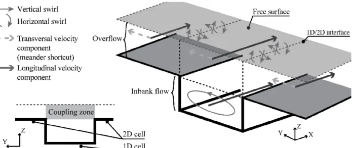
Figure 1: Proposed model for the flow in a 2D-cell and its included 1D-cell. Left: definition of the cells and the coupling zone; right: flow hypotheses – uniform distribution of the velocity over the vertical, identical transverse velocity components in the 1D- and 2D-cell, mean of the transversal velocity in the bottom of the main channel equal 0 due to the vertical swirl and formation of horizontal swirls due to velocity shear along
the 1D/2D interface.
The proposed model involves 1D-cells to represent canalized flow (such as main river channels or streets in urban area) within a classical unstructured 2D mesh as in Sobek-1D2D [3]. On the 1D-cells, the flow is considered follow the direction of the main channel.
To achieve these proposed goals, several hypotheses have been made on the geometry (see Figure 1): - (i) each 1D-cell is included in a 2D-cell,
- (ii) the bottom elevation is the same on each side of the main channel; on the flow:
- (iii) the water elevation is the same on a 2D-cell and its included 1D-cell,
- (iv) the velocity component in the longitudinal direction is uniform over a vertical line, - (v) the transversal velocity component is constant in the 2D and the coupling zone; and on the flow behaviour:
- (vi) the velocity shear between the 1D and the 2D flows leads to the apparition of swirls and thus to a momentum transfer that can be estimated using Bousmar and Bertrand’s formulation,
- (vii) the velocity shear between 1D and coupling zone leads to a vertical swirl that can be taken into account via head losses coefficient.
II.2 Governing equations
The governing equations are established using a mass and momentum balance over a control volume containing both a 1D- and 2D-flow. The parts of the global equations corresponding to each domain are separated, thus yielding an exchange term T. On both the 1D- and the 2D-control volumes, the differential equations can be written as:
T S G F U ± = ∂ ∂ + ∂ ∂ + ∂ ∂ y x t (1)
(
)
(
)
∂ ∂ + − ∂ ∂ + − = + = + = = y gh S S h g x gh S S h g h g h r h qr r h qr h g h q q r q h x f x x f x φ φ φ φ φ φ φφ φ φ φ φ φ φ φ 2 , , 0 2 , , 0 2 2 2 2 2 1 2 1 0 2 1 2 1 G S F Uwhere U is the vector of the conserved variable, F and G are the flux functions, S the source term, g the gravitational acceleration, h the water depth, q (resp. r) the unit-discharge in the x (resp. y) direction,
x
S0, (resp. S0,y) the bottom slope in the x (resp. y) direction, Sf,x (resp. Sf,y) the friction slope in the x
(resp. y) direction. In 2D, the term φ stands for the porosity [6], [7] and represents the fact that the whole 2D-cell is not available for 2D-flow (since one part is used for the 1D-flow). In 1D, φ corresponds to the channel width.
By hypothesis, when the 1D equations are written in the referential associated to the channel (i.e. the x
axis is in the same direction than the 1D-channel), the flux function G, the bottom slope S0,y and the partial derivative of the width ∂φ ∂y are nil.
III 2. NUMERICAL METHOD
When the equations that have to be solved involve source terms, the time splitting method is generally used. This method proposes to solve the whole problem over each time step as several simpler sub-problems which are solved using the most appropriate numerical technique [8]. The source and transfer terms are split into four physical and two equilibrium terms:
[
p f]
[
l m t]
y x t S S S T T T G F U + + ± + + = ∂ ∂ + ∂ ∂ + ∂ ∂ 0 (2)Equation (2) is solved using the following algorithm:
- solve the conservative part of the equations with the source terms corresponding to the topography (i.e. the bottom slope S0 and the porosity or channel width variation Sp),
- take the friction terms Sf into account,
- take into account the longitudinal momentum transferTl.
These three steps correspond to the solution of the physical part of the model. To guarantee that the model hypotheses are verified, two balancing steps are performed:
- mass balance between the 2D- and its associated 1D-cell through the transfer term Tm to respect
hypothesis (iii),
- transversal momentum balance between the cells throughTt.
After each step of the algorithm, an intermediate value of the conserved variable is estimated: n,c
U , n,f
U , n,l
U , n,m
U and n,t
III.1 Conservation part of the equations
The conservative part of the equations including the geometrical source terms is solved using a finite volume approach. The equations are discretized as follow:
( )
∑
∈ + + + + ∆ − = i N j i n ij ij n if ij i n i n i L A t 12 2 1 1 S F P U U (3)where the subscripts i denotes either a 1D- or a 2D-cell and ij the interface between the cells i and j (being respectively on the left- and right-hand side of the interface); ∆t is the computational time step, Ai the plan
view area of the cell i, N
( )
i the set of the neighbouring cells of the cell i, Lij the width of the interface ij, n iU the average value of Uover the cell i at the time n, n+12
ij
F the average value of the flux at the interface ij over the time step n,n+1, Pij the matrix that transforms the variable in the global coordinate system into the local
coordinate system attached to the interface and
i n ij +12
S is the contribution of the source terms to the cell i computed from U between the cells i and j.
In the proposed software, the computation of both the n+12 ij F and i n ij +12
S terms is performed using the HLLC solver [9], allowing to estimateUafter the first step: Un,c.
III.2 Integration of the friction term
The friction term Sf is computed by solving the following ordinary differential equation in each direction of space: r R h K r q g t r q R h K r q g t q y h y x h x 3 1 , 2 2 2 2 3 1 , 2 2 2 2 d d d d =− + =− + (4)
where Kx and Rh,x are the Strickler coefficient and the hydraulic radius in the x direction (respectively Ky
and Rh,y in the y direction). Over each 2D-cell and in the transversal direction of the 1D-cell, the hydraulic
radius is approximated with the water depth. In the main direction of the 1D-cell, the full expression of the hydraulic radius is taken into account. The methodology used to calculate the hydraulic radius is justified in [10]. The intermediate state Un,f involves an intermediate value of the components of the unit-discharge that
are calculated by solving the equations (4):
( ) ( )
( )
( ) ( )
( )
∆ + − = ∆ + − = t R h K r q g r r t R h K r q g q q y h c n y c n c n c n f n s h c n x c n c n c n f n 3 1 , 2 , 2 2 , 2 , , , 3 1 , 2 , 2 2 , 2 , , , exp exp (5)III.3 Longitudinal momentum transfer
After the solution of the conservative part of the equations and the integration of the source terms due to geometry and friction, the longitudinal momentum transfer is performed. The hypothesis (vi) of the model states that the shear due to the difference of longitudinal velocity between the 2D- and the 1D-cell generates horizontal swirls. The average mass exchanged through the interfaces between the 2D-cell and its associated 1D-cell is nil. However, the exchanged yields a momentum transfer. The formulation proposed by Bertrand [11] and Bousmar [12] is used. The unit discharge qlat generated by the swirls is estimated by:
(
)
nf D f n D f n D lat u u h q =ψ 1, − 2, cosβ 2, (6)where β is the angle between the main channel direction and the interface (that is, between the 2D-cell and its associated 1D-cell), nf
D
h2, is the water depth within the 2D-cell at the end of the friction step,
f n
D
u1, is the
longitudinal component of the velocity at the end of the friction step on the 1D-cell (respectively nf D
u ,
2 on the
2D-cell) and ψ is a proportional factor. Bousmar has conducted experiments that show that the ψ factor is not influenced by the geometry and is therefore taken equal to 0.016.
As the unit-discharge generated by the swirls can be calculated, it is possible to determine the water volume that is exchange between the 1D- and 2D-cells and therefore to transfer the momentum contained within this volume, leading to the estimate n,l
U .
III.4 Mass balance
At the end of the previous step, the value of the conserved variable n,l
U may not respect the hypothesis used to build the model. Therefore a mass balance is performed to insure that the water surface elevation is the same in the 2D-cell and its associated 1D-cell (except if the water surface elevation in the 1D-cell is below the bottom elevation in the corresponding 2D-cell). It can be shown that the water surface elevation after the mass balance step should be equal to the mean of the water surface elevation in both cell weighted by the plan view area of each cell:
D D l n D D l n D D m n A A z A z A z 2 1 , 2 2 , 1 1 , + + = (7)
The momentum contained in the volume transferred from one cell to the other is also transferred to insure that the momentum balance on each cell is respected in the estimate ofUafter the mass balance step: n,m
U .
III.5 Transversal momentum equilibrium
By construction, the transverse component of the velocity is the same on the 1D- and the 2D-cells. The transversal component of the velocity should therefore be equal to:
m n D D m n D D m n D m n D D m n D m n D D t n h A h A v h A v h A v , 2 2 , 1 1 , 2 , 2 2 , 1 , 1 1 , + + = (8)
The flow in the transverse direction being known, the water volumes exchanged across the interface between the 2D- and its associated 1D-cell are:
t v h L V t v h L V t n t n D R R t n t n D L L ∆ = ∆ = , , 2 , , 2 (9)
where LL is the length of the interface between the 2D- and its associated 1D-cell corresponding to the left
bank (respectively LR for the right bank). The momentum contained in the mass volumes that flow through
the interfaces are also transferred to insure the respect of the momentum balance over each cell.
The vertical swirls generated by the over flow in the 1D-cell are responsible for a headloss. However, the headloss coefficient law that may depend on both the geometry and the flow have not yet been estimated. Therefore, the current version of proposed software SW12D does not take this headloss into account.
IV 3. COMPUTATIONAL EXAMPLES
The proposed 1D-2D model aims to reproduce the results obtained with a classical 2D software with a reduced computation time. Also, the proposed model should be able to correctly represent the phenomena that involve momentum transfer between the main channel (represented by the 1D-cells) and the overbank (corresponding to the 2D-cells). To highlight the performance of the proposed model, a comparison of the results produced by various numerical softwares (SW12D and SW2D) with experimental data has been carried out. A comparison has also been performed on a real-world test case corresponding to an engineering study.
IV.1 Sinuous experiment
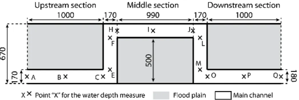
The sinuous experiment consists in a topography with four 90° bends (Figure 2). The bottom elevation of the floodplain is 0.1 m higher than the main channel. Upstream, a permanent discharge is imposed (5 l s-1). At the downstream end, the water depth is imposed using a wear such as keeping the flow only in the main channel (“Inbank experiment”) or having overflow (“Flood experiment”). In the two experiments, both the water depth and the flow velocity have been measured.
Figure 2: Plan view of the configuration used for the sinuous experiment. Dimensions in mm. The bottom elevation is nil in the main channel and equal to 0.1 m in the main channel.
For the “Inbank experiment”, the measured water depths are compared to the numerical results produced by both SW12D and SW2D (see Figure 3a). In the SW12D mesh’s cross-section, there is only one 1D-cell to represent the main channel included in a 2D-cell that represents the overbank. For SW2D, rectangular cells (about 1 cm2) are used. The water depths produced by SW12D are in adequation with the experimental values whereas SW2D does not manage to reproduce the experiment, even with a fine mesh. However, the location of the headloss due to bends are well-located by both softwares. The overestimation of the water depth by SW2D has been explored and is probably due to the downstream boundary condition. Since the aim of the current article is to present the SW12D coupling methodology, no further investigation on SW2D have been carried out. Moreover, the computation time is 906 s with SW2D and only 46 s with SW12D, corresponding to a time reduction by factor 19.7 for more accurate results.
Figure 3a : Water depth for the “Inbank Experiment” Figure 3b : Velocity ratio for the “Flood experiment” Figure 3: Comparison of the surface elevation and velocity ratio measured and calculated by SW12D and SW2D.
For the “Flood experiment”, the measured water depths are correctly reproduced by both models. The ratio of the velocity in the main channel to the velocity in the overbank flow is compared between the experiment and the numerical data (see Figure 3b). In this case, SW12D better reproduces the velocity ratio compared to SW2D. This may be explained by the hypothesis on the repartition of the experimental discharge between the main channel and the overbank that should have been made for the determination of the upstream condition. However, this cannot be verified without further experiment. For this experiment, the use of SW12D instead of SW2D allows a time reduction by 81.
IV.2 Real world test case
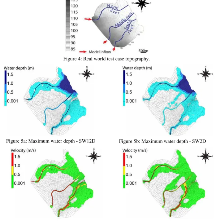
A real world configuration has also been used to compare SW12D and SW2D. The topography has been provided by Ginger Environment and Infrastructures and corresponds to a small portion of a real engineering study area. The modelled area presents three rivers called (from north to south): the North river, the Middle river and the South river (Figure 4).
Figure 4: Real world test case topography.
Figure 5a: Maximum water depth - SW12D Figure 5b: Maximum water depth - SW2D
Figure 5c: Maximum velocity - SW12D Figure 5d: Maximum velocity - SW2D Figure 5: Comparison of the maximum water depth and velocity computed by SW12D and SW2D. The overall hydrodynamic comportment remains the same with both models. However, SW2D identify:
- a flow from the Middle river to the downstream of the North river with both a small discharge and depth (that appears on Figure 5b and 5d due to a threshold effect)
- a flow from the middle of the South river to the downstream of the Middle river. Locally, this flow leads to two different hydrodynamical comportments. However, both comportments are physically coherent. It is impossible to state if one is more representative of the real world flow.
It is difficult to compare in detail the results obtained with both softwares principally because of the complexity of any real world configuration. However, the results obtained are very similar with a reduction of the computation time by 16 using SW12D instead of SW2D.
V CONCLUSION
A new 1D-2D coupling methodology has been developed to take into account the mass and momentum exchanges between the 1D- and the 2D-model. This represents a significant improvement as the momentum
transfer is generally neglected in the existing 1D-2D models. Accounting for momentum transfer in the governing equation allows for a correct representation of the phenomena such as meander shortcuts.
The validation of the proposed methodology, implanted in the SW12D software, has been realized on numerous numerical test cases. The comparison of the SW12D results with the classical 2D software SW2D highlights a significant improvement of the modelling of momentum transfer between the main channel and the overbank linked phenomena. Similar comparison with the 1D software HEC-RAS (not presented here) leads to the same conclusion [10, [13]. Moreover, the use of SW12D allows for a substantial reduction of the computation time in comparison with a classical bidimensional software.
VI ACKNOWLEDGEMENTS
This research has been partly carried out during a Ph. D. Thesis funded by GEI (Ginger Environnement et Infrastructures), a Ginger Group Company. The experimentats have been carried out at the National Superior School of Agronomy of Montpellier (SupAgro Montpellier).
VI.1 REFERENCES AND CITATIONS
[1] US Army Corps of Engineers, Hydrologic Engineering Center (2006). HEC-RAS, River Analysis System –
User’s Manual.
[2] Altinakar, M. S., Miglio, E. & Wu, W. (2008). Coupling 1D-2D shallow water models for simulating floods due to overtopping and breaching of levees. In Proceedings of the 8th World Congress on
Computational Mechanics (WCCM8) – 5th European Congress on Computational Methods in Applied Sciences and Engineering (ECCOMAS 2008), Venice (Italy).
[3] Dhondia, J. F. & Stelling, G. S. (2002). Application of one-dimensional – two-dimensional integrated hydraulic model for flood simulation and damage assessment. In Proceedings of the 28th ICCE 2002,
ASCE, Cardiff, 2002.
[4] Erpicum, S., Archambeau, P., Dewals, B. J., Detrembleur, S. & Pirotton, M. (2006). Fluid-structure interaction modelling with a coupled 1D-2D surface flow solver. In Proceedings of Riverflow 06,
Lisbon (Portugal), 2006.
[5] Erpicum, S., Archambeau, P., Dewals, B. J., Detrembleur, S. & Pirotton, M. (2006). 1D and 2D solvers coupling for free surface flow modelling. In Proceedings of the 7th International Conference on
Hydroinformatics, HIC 2006, Nice, France, 2006.
[6] Finaud-Guyot, P., Delenne, C., Lhomme, J., Guinot, V. & Llovel, C. (2010). An approximate-state Riemann solver for the two-dimensional shallow water equations with porosity. International Journal
for Numerical Methods in Fluids.62, 1299-1331.
[7] Lhomme, J. & Guinot, V. (2007). A general approximate-state Riemann solver for hyperbolic systems of conservation laws with source terms. International Journal for Numerical Methods in Fluids, 53, 1509-1540.
[8] Guinot, V. (2003). Godunov-type schemes, An introduction for engineers. Elsevier.
[9] Guinot, V. & Soares-Frazao, S. (2006). Flux and source term discretization in two-dimensional shallow water models with porosity on unstructured grids. International Journal for Numerical Methods in
Fluids, 50, 309-345.
[10] Finaud-Guyot, P. (2009). Macroscopic flood modelling: Taking into account directional flows and main channel – floodplain transfer. PhD thesis, Université Montpellier 2. (In French).
[11] Bertrand, G. (1994). Le calcul d’axes hydrauliques dans les rivières à plaines inondables. Technical report, Ministère Wallon de l’Equipement et des Transports, D. 213, Chatelet, Belgium. In French. [12] Bousmar, D. (2002). Flow modelling in compound channels. PhD thesis, Université Catholique de
Louvain.
[13] Finaud-Guyot, P., Delenne, C., Guinot, V. & Llovel, C. (2011). 1D-2D coupling for river flow modelling. Comptes rendus de l’académie des Sciences. (Accepted)