Extracting low frequency climate signal from GRACE data

HAL Id: hal-00330780

https://hal.archives-ouvertes.fr/hal-00330780

Submitted on 4 Oct 2006

HAL is a multi-disciplinary open access

archive for the deposit and dissemination of

sci-entific research documents, whether they are

pub-lished or not. The documents may come from

teaching and research institutions in France or

abroad, or from public or private research centers.

L’archive ouverte pluridisciplinaire HAL, est

destinée au dépôt et à la diffusion de documents

scientifiques de niveau recherche, publiés ou non,

émanant des établissements d’enseignement et de

recherche français ou étrangers, des laboratoires

publics ou privés.

Extracting low frequency climate signal from GRACE

data

O. de Viron, I. Panet, M. Diament

To cite this version:

O. de Viron, I. Panet, M. Diament. Extracting low frequency climate signal from GRACE data.

eEarth, 2006, 1 (1), pp.9-14. �hal-00330780�

www.electronic-earth.net/1/9/2006/ © Author(s) 2006. This work is licensed under a Creative Commons License.

eEarth

Extracting low frequency climate signal from GRACE data

1_{Institut de Physique du Globe de Paris (associated with the CNRS and the University Paris 7), Paris, France} 2_{LAREG, Institut G´eographique National, Marne-La-Vall´ee, France}

Received: 27 March 2006 – Published in eEarth Discuss.: 15 May 2006

Revised: 29 August 2006 – Accepted: 28 September 2006 – Published: 4 October 2006

Abstract. For more than four years, the GRACE pair of

satellites have been orbiting the Earth, monitoring the time variable mass distribution for scales ranging from regional to global. The GRACE data have been released for a broad scientific community and sets of gravity fields are available. This paper shows that there are evidences at interrannual time scales for the presence of ENSO signal in the data, strongly correlated with the hydrological mass distribution, and also similar to the expected hydrological signature asso-ciated with the ENSO cycle. This signal dominates, at global scale, the one associated with geodynamic sources.

1 Introduction

The GRACE satellite mission gives access to the temporal variability of the gravity field at global scale. It is now in progress for more than three years, and 43 spherical harmon-ics developments of the gravitational potential fields, dis-tributed by the Center for Space Reasearch (CSR, Austin, Texas) are now available for analysis (Tapley et al., 2004). The product are spherical developments of the geopotential up to degree 120, from April 2002 to February 2006.

Monitoring the gravity field as a function of time allows to follow the changes in mass distribution within the Earth tem. This is of vital importance for studying the climate sys-tem, as it is very difficult to monitor, at global scale, the mass redistribution inside the superficial fluid layers, a mandatory task for improving our knowledge of the Earth climate. The GRACE data have already been shown successful in test-ing hydrological models at the annual (Tapley et al., 2004; Ramillien et al., 2004; Rowlands et al., 2005) and interran-nual (Andersen and Hinderer, 2005) periods. Another inter-est of the GRACE mission is the detection of mass changes

Correspondence to: O. de Viron

(deviron@ipgp.jussieu.fr)

due to tectonics (Mikhailov et al., 2004; Sun and Okubo, 2004; Han et al., 2006; Diament et al., 20061). However, such signals are globally weaker than those related to fluid envelopes. Therefore, it is necessary to substract the climate signal from the GRACE data in order to isolate the signal of geodynamic origin.

We analyze GRACE data in order to investigate the low frequency signal and its physical meaning. More specifi-cally, we expect a contribution from the El-Ni˜no Southern Oscillation (ENSO), a global signal in the climate system at interannual timescale. ENSO impact on the hydrology has been reported (e.g., Donders et al., 2005; Foley et al., 2002; Whiting et al., 2004), in various locations. Consequently, we can expect it to be observable in the data as a mode of com-mon variability of the mass distribution at global scale over the continents. The ENSO impact on the ocean is known to be mainly steric and is consequently not expected to be asso-ciated with a noticable gravity signal. To search for an ENSO signal in the GRACE data, the Empirical Orthogonal Func-tion (EOF) decomposiFunc-tion is particularly well-suited. First developed for atmosphere science study, this method decom-poses a given time varying field in modes of variabilities, in such a way that an important part of the variance can be re-trieved from only a few modes, each mode being a time series associated with a geographical distribution. It is thus very ef-ficient at retrieving common variability from noisy signals.

The paper is organized as follows. In Sect. 2, we explain how we prepare the data prior to analysis. In Sect. 3, a very short explanation about the EOF method is given. Section 4 is devoted to the EOF analysis of the space gravity data, and to the discussion of the results. In Sect. 5, we look for the ENSO signature in an hydrology model simulation over the

1_{Diament, M., King, G., Michailov, V., Panet, I., and de Viron,}

O.: Space gravity reveal subduction in the Andaman sea caused by the giant Sumatra-Andaman Earthquake, Geophys. Res. Lett., submitted, 2006.

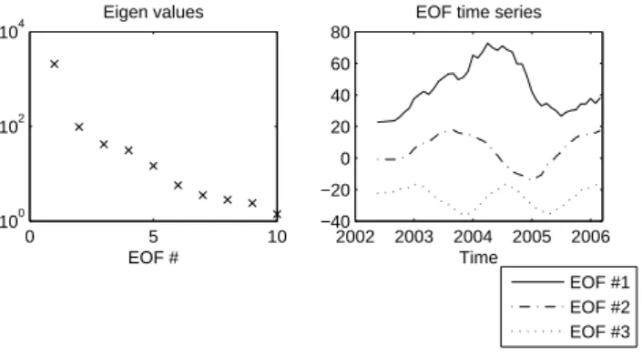
10 O. de Viron et al.: Low frequency signal in grace data 0 5 10 100 102 104 Eigen values EOF # 2002 2003 2004 2005 2006 −40 −20 0 20 40 60 80 Time EOF time series

EOF #1 EOF #2 EOF #3

Fig. 1. EOF decomposition of the CSR GRACE data: the left panel

shows the eigenvalues, which are a measure of the variance ex-plained by the EOF, and the right panel shows the time series as-sociated with the EOF, for the three first modes. The first one has been divided by 3, and an arbitrary shift has been added to separate the time series.

last 20 years. Discussion and concluding remarks are given in Sect. 6.

2 Data used and their preparation

The CSR products, with 43 monthly solutions between April 2002 and February 2006 and a missing field in June 2003, have been used for this study. The spatial fields have been reconstructed on 2.5-degree by 2.5-degree grids, from the spherical harmonics development, up to degree 50, with half a Hamming window progressively cutting off from degree 30. In this study, since we focus on continental area, the ocean grid points are not analyzed. All the computations were done using the geoid topography.

We fit and removed the seasonal signal (composed of an annual, and semi-annual oscillation) for each grid point, over the existing 4 years of data. Then, the results were smoothed with a 4-month window, in order to emphasize the low fre-quency signal.

We assume that the internannual signal has an hydrologi-cal origin, consequently, we finally keep only continent data, as this is where the hydrology signal is, and we used the land dynamics (LaD) hydrology for comparison (see Milly and Shmakin, 2002). The LAD data are available from January 1980 to May 2005, with a 1 degree resolution. For compar-ison with the GRACE results, we converted the mass fields to geoid, using the formula of Swenson and Wahr (2002), at the same 2.5×2.5 resolution, removed the annual signal, and smoothed them with a 4-month window.

To compare with the ENSO, we used the Southern Oscil-lation Index (SOI, i.e. scaled difference of pressure anomaly between Darwin and Tahiti, see Trenberth, 1984) smoothed with the same 4-month window as the other data sets.

3 Methods used: the EOF and SVD decompositions

To characterize the spatio-temporal variability of the grav-ity field, we choose to use the EOF decomposition. This method is explained in details for instance in Preisendorfer (1988). The EOF decomposition represents a space-time data set (xi(tj), i=1, ..., n, j =1..., m) in terms of a given

num-ber N of variability modes, each of which is a time series Ak(t )and a geographical distribution Xk(i), with

xi(tj) = N

X

k=1

Ak(tj)Xk(i) (1)

These modes are obtained from the eigenvalue decompo-sition of the covariance matrix R=FTF, with the matrix Fij=xi(tj). The eigenvalues represent the variance

ex-plained by the mode of variability, and the eigenvectors, of-ten called EOF as they are orthogonal, represent the space distribution of the modes. The modes are sorted by decreas-ing eigenvalue, so that the first mode explains more variance than any other. The time variability associated with each EOF can be retrieved by projecting the matrix F on the eigen vector.

To retrieve the modes of common variability between two datasets, we used the Singular Value Decomposition (SVD). This method is classically applied when two combined data fields (xi(tj) and yi(tj), i=1, ..., n, j =1..., m) are to be

analysed. The method decomposes the signal into time series associated with pairs of spatial patterns. Each pair explains a fraction of the covariance between the two fields. The co-variance matrix is then defined as

C = xTy (2)

A singular value decomposition is then performed on the co-variance matrix

C = U LVT (3)

The columns of U are the eigenvectors for x, and the columns of V those of y. Similarly as what was done for the EOF, each data field is then projected on the eigenvectors in order to obtain the time series.

4 EOF decomposition of the GRACE data

We performed an EOF decomposition on the continent geoid data, using the CSR data. The results are shown on Fig. 1. The left panel displays the eigen value as a function of the EOF number. Most of the variance is explained by the first two modes. The right panel shows the time series of the three first EOF modes. Note that the first one has been divided by 3, in order to show them all on the same plot. The two first modes are interannual, the third is nearly annual, and will not be discussed here. Note that the seasonal cycle has been removed, otherwise this would be the first mode. The

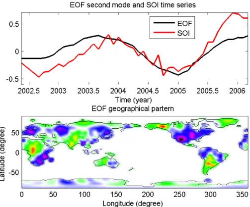
Fig. 2. Top panel: First EOF time series computed on the CSR GRACE data, and scaled SOI. Bottom panel: Geographical pattern associated

with the first EOF. The results have to be understood as the factor multiplying the time series. Warm colors indicate places where the mass distribution is in phase with the time series, and cold colors indicate places where it is out of phase.

geographical pattern of the first mode appears to be the pro-jection on the continent mask of a degree 2 order 0 spherical harmonics, and is linked to the variation of the dynamic flat-tening, J2, of the Earth. Considering its magnitude and its

very clean geographical pattern, we thus suspect it to be not related to any geophysical process, and we will not further discuss it.

The ENSO is a very important signal in the climate sys-tem, and it is global scale. Number of studies have reported impact of the ENSO on the pluviometry and on the hydrol-ogy, locally and globally (e.g. Dilley and Heyman, 1995; Cayan et al., 1999; Soden, 2000). Consequently, we expect an ENSO associated signal to be found as a common mode of variability in the mass distribution at the Earth surface, com-ing from mass variation in hydrology. In Fig. 2, we display the time series of the second EOF and the SOI. The correla-tion coefficient between the two is equal to 0.74. To assess the significance of this coefficient, we need to estimate the number of degrees of freedom of the system. This number is classically obtained, for time series, by dividing the length of the signal by the decorrelation time, i.e. the lag for which the auto-correlation drops below e−1. We found that there are 6 degrees of freedom in our signal, which makes the computed correlation coefficient significant at more than 98%. This supports our hypothesis that the second EOF mode is related to the ENSO cycle. On the bottom panel, we display the

ge-ographical pattern associated with this mode. We discuss it here below, in comparison with the hydrological signal.

5 EOF decomposition of the LAD data

In order to test whether this mass variation is due to a conti-nental hydrology signal, we applied the same analysis to the hydrology data. In Fig. 3, we display the results from the EOF analysis applied to the geoid variations computed out of the LAD data, of which the simulation ends in May 2005. We limited our analysis to the last 20 years, as in the first 5 years, the simulation does not seem to be stabilized yet.

The time series of the first mode, in the first few years, looks like the model is still stabilizing. If we remove the first 3 years of hydrology data, this mode disapears, and the previously second mode becomes the first one.

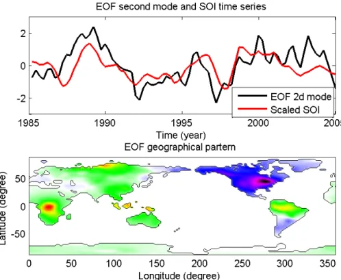
As for the GRACE products, the second EOF time series is well correlated with the SOI. The correlation coefficient is 0.59, and is significant at the 99.5% level, considering that there are 15 degrees of freedom. The bottom panel repre-sents the mass distribution which would be associated with the ENSO. The two geographical patterns have some impor-tant common features. In particular, the rather negative mass anomalies on the North America are present and in phase on both EOF, so is the positive anomaly on Eurasia, although the GRACE data show some additional smaller scale negative

12 O. de Viron et al.: Low frequency signal in grace data

Fig. 3. Left top panel: First two EOF time series and scaled SOI of the LAD hydrology model. Bottom panel: Geographical pattern

associated with the first EOF.

Fig. 4. Covariance Map of the hydrology geoid and SOI. For each

grid point, the colorscale represents the covariance between the time variation of the geoid height from hydrology at the point and the SOI. Cold colors indicate anticorrelation, and warm color indicate correlation. The zero-covariance has been set to white.

anomalies. The anomaly on central Africa appears in both maps. The existence of differences between the two maps are not surprising as, with only 4 years of data, we cannot sider that we have a very good sampling of the El-Ni˜no con-figuration. In addition, no major Ni˜no/Ni˜na event occured during the GRACE era, and it is quite possible that the hy-drology signal somewhat differs when there is a major event. Nevertheless, it seems reasonable, considering that both the time series agree, and that the geographical patterns have im-portant similarities, to assume that the signal we obtain by the EOF analysis of the GRACE data is due to an hydrological signal.

To confirm this hypothesis, we computed a Singular Value Decomposition (SVD) of the two set fields. The results we obtained showed that the SVD modes are similar both in time series and in geographical patterns to the one obtained by the EOF.

6 ENSO signature in the LAD hydrology

We have shown that there are low frequency signals in the GRACE data, and in the LaD hydrology, which have some important similarity in the geographical pattern. We have also shown that the time variability is well correlated with the SOI for the same epoch. We used the whole 20 years of LaD data, to find the hydrology signature of the ENSO. This will close the loop, allowing to test to which extend the EOF mode that we found correlated with the SOI is indeed

the hydrology signal associated with the ENSO. To this end, we computed a map of the covariance between the SOI and the hydrology.

The results are displayed on Fig. 4. As shown by compar-ison with Fig. 3, the geographical patterns are quite similar, which shows that the EOF decomposition of the hydrology data has retrieved the ENSO-associated signal, and not only a small fraction of it. This strongly supports that the signal we have retrieved from the GRACE data is indeed associated with the ENSO cycle.

7 Conclusions

Our aim was to investigate the interannual signal in the GRACE data, and in particular, we thought likely that the ENSO cycle, which is the largest global climate mode at in-terannual period, would be present in the GRACE data. Of course, finding a signal which is supposed to be at interan-nual period with a few year data is very challenging, but we think we found some convincing indications that there are long term variability present in the GRACE data, and that an important part of it comes from the hydrological signal associated with the ENSO cycle.

We found 2 modes explaining most of the variance of the low frequency GRACE signal. The first one seems unphysi-cal, as it is purely a degree two order zero spherical harmonic (related to the variation of the dynamic flattening, J2, of the

Earth). The second one is associated with the ENSO. The first mode in the LAD data also seems unphysical, as the model seems to have not finished its stabilisation yet. The second mode exhibits a time series significantly correlated with the SOI, and a reasonably similar geographical pattern is also present in the hydrology data. Moreover, the geo-graphical pattern associated with this mode is typical of the hydrological signature of the El-Ni˜no.

To conclude, we suggest that GRACE have captured, dur-ing those four years of available data, signal comdur-ing from long term variability in the climate system, more precisely associated with the ENSO cycle. This seems to be the domi-nant signal retreived at low frequency by GRACE. Extracting the mass variation associated with global scale phenomenon as the ENSO cycle is of broad interest for many scientists of the Earth sciences. Global time variable gravity missions are unique opportunities to provide a global information on the water distribution, which is necessary to constrain global circulation models of the climate system.

These results also show the efficiency of the EOF method to retrieve consistent signal, for instance of climate origin, in the GRACE data. It also shows how this signal can be separated from signal of Earth interior origin, a mandatory task to use GRACE data to study geodynamics.

Acknowledgements. This study was supported by CNES. This

paper is the IPGP contribution #2172. The authors thank two anonymous referees for helpful comments on the manuscript.

Edited by: T. Van Dam

References

Andersen O. B. and Hinderer, J.: Global inter-annual changes from GRACE: Early results , Geophys. Res. Lett., 32, L01402, doi:10.2029/2004GL020948, 2005.

Biancale, R., Lemoine, J.-M., Balmino, G., Bruinsma, S., Perosanz, F., Marty, J.-C., Loyer, S., and G´egout, P.: 3 years of geoid variations from GRACE and LAGEOS data at 10-day intervals over the period from July 29th, 2002 to March 24th, Data CD, CNES/GRGS product, 2005.

Cayan, D. R., Redmond, K. T., and Riddle, L. G.: ENSO and Hydrologic Extremes in the Western United States, J. Climate, 12(9), 2881–2893, 1999.

Dayana, U. and Lambb, D.: Global and synoptic-scale weather patterns controlling wet atmospheric deposition over central Eu-rope, Atmos. Environ., 39, 521–533, 2005.

Dilley, M. and Heyman, B. N.: ENSO and disaster: Droughts, floods and El Ni˜no-Southern Oscillation warm events, Disasters, 19(3), 181–193, 1995.

Donders, T. H., Wagner, F., Dilcher, D. L., and Visscher, H.: Mid- to late-Holocene El Ni˜no-Southern Oscillation dynamics reflected in the subtropical terrestrial realm, Proc. Nat. Ac. Sci. USA, 102(31), 10 904–10 908, 2005.

Foley, J. A., Botta, A., Coe, M. T., and Costa, M. H.: El Ni˜no-Southern Oscillation and the climate, ecosystems and rivers of Amazonia, Global Biogeochem. Cycles, 16(4), 1132, doi:10.1029/2002GB001872, 2002.

Han, S., Jekeli, C., and Shum, C. K.: Time-variable aliasing ef-fect of ocean tides, atmosphere, and continental water mass on monthly mean GRACE gravity field, J. Geophys. Res., 109, B04403, doi:10.2029/2003JB002501, 2004.

Han, S., Shum, C. K., Bevis, M., Ji, C., and Kuo, C.: Crustal Di-latation Observed by GRACE After the 2004 Sumatra-Andaman Earthquake, Science, 313(5787), 658–662, 2006.

Mikhailov, V., Tikhotsky, S., Diament, M., Panet, I., and Ballu, V.: Can tectonic processes be recovered from new gravity satellite data?, Earth Planet. Sci. Lett., 228, 281–297, 2004.

Milly, P. C. D. and Shmakin, A. B.: Global modelling of land water and energy balances. Part I: The land dynamics (LaD) model, J. Hydrometeol., 3(3), 283–299, 2002.

Mo, K. C. and Livezey, R. E.: Tropical-Extratropical Geopotential Height Teleconnections during the Northern Hemisphere Win-ter, Mon. Wea. Rev., 114(12), 2488–2515, doi:10.1175/1520-0493(1986)114, 1986.

Preisendorfer, R. W.: Principal Component Analyses in Meteorol-ogy and Oceanography, Elsevier, 444 p., 1988.

Rowlands, D. D., Luthcke, S. B., Kolsko, S. M., Lemoine, F. G. R., Chinn, D. S., McCarthy, J. J., Cox, C. M., and Anderson, O. B.: Resolving mass flux at high spatial and temporal resolution using GRACE intersatellite measurements, Geophys. Res. Lett., 32, L04310, doi:10.1029/2004GL021908, 2005.

Ramilien, G., Cazenave, A., and Brunau, O.: Global time varia-tions of hydrological signals from GRACE satellite gravimetry, Geophys. J. Int., 158, 813–826, 2004.

Swenson, S. and Wahr, J.: Methods for inferring regional surface-mass anomalies from Gravity Recovery and Climate Experiment

14 O. de Viron et al.: Low frequency signal in grace data

(GRACE) measurements of time-variable gravity, J. Geophys. Res., 107(B9), 2193, doi:10.1029/2001JB000576, 2002. Sun, W. and Okubo, S.: Coseismic deformations detectable by

satellite gravity missions: A case study of Alaska (1964, 2002) and Hokkaido (2003) earthquakes in the spectral domain, J. Geo-phys. Res., 109, B04405, doi:10.1029/2003JB002554, 2004. Soden, B. J.: The Sensitivity of the Tropical Hydrological Cycle to

ENSO, J. Climate, 13(3), 538–549, 2000.

Tapley, B. D., Bettadpur, S., Ries, J. C., Thompson, P. F., and Watkins, M. W.: GRACE Measurements of Mass Variability in the Earth System, Science, 305, 503–503, 2004.

Trenberth, K. E.: Signal versus Noise in the Southern Oscillation, Mon. Wea. Rev., 112, 326–332, 1984.

Whiting, J. P., Lambert, M. F., Metcalfe, A. V., Adamson, P. T., Franks, S. W., and Kuczera, G.: Relationships between the El-Ni˜no Southern Oscillation and spate flows in southern Africa and Australia, Hydrol. Earth Syst. Sci., 8(6), 1118–1128, 2004.