A satellite-based method for estimating global oceanic DMS and its application in a 3-D atmospheric GCM

HAL Id: hal-00203720

https://hal.archives-ouvertes.fr/hal-00203720

Submitted on 13 Jan 2020

HAL is a multi-disciplinary open access

archive for the deposit and dissemination of

sci-entific research documents, whether they are

pub-lished or not. The documents may come from

teaching and research institutions in France or

abroad, or from public or private research centers.

L’archive ouverte pluridisciplinaire HAL, est

destinée au dépôt et à la diffusion de documents

scientifiques de niveau recherche, publiés ou non,

émanant des établissements d’enseignement et de

recherche français ou étrangers, des laboratoires

publics ou privés.

A satellite-based method for estimating global oceanic

DMS and its application in a 3-D atmospheric GCM

Sauveur Belviso, Cyril Moulin, Laurent Bopp, Emmanuel Cosme, Elaine

Chapman, Kazushi Aranami

To cite this version:

Sauveur Belviso, Cyril Moulin, Laurent Bopp, Emmanuel Cosme, Elaine Chapman, et al.. A

satellite-based method for estimating global oceanic DMS and its application in a 3-D atmospheric GCM.

Emissions of atmospheric trace compounds, Springer, pp.305-332, 2004,

�10.1007/978-1-4020-2167-1_8�. �hal-00203720�

A satellite-based method for estimating global oceanic

DMS and its application in a 3-D atmospheric GCM

Sauveur Belviso, Cyril Moulin, Laurent Bopp, Emmanuel Cosme, Elaine Chapman and Kazushi Aranami

1. INTRODUCTION

In order to assess in three-dimensional atmospheric models the climate effects of anthropogenic sulphate aerosols, it is necessary not only to compute spatial and temporal distributions of anthropogenic sulphate, but also to simulate spatially and temporally the emission, transport and transformation of natural sulphur gases and aerosols emitted at the Earth's surface. Jones et al. (2001) recently obtained a value of - 1.9 W m2 for the effect of anthropogenic sulphate aerosol on cloud albedo and on precipitation efficiency (the 'indirect' sulphate aerosol forcing effect), and demonstrated in a sensitivity test that doubling oceanic dimethylsulphide (OMS) emission fluxes reduced the indirect effect by over 25%. Thus, changes in marine DMS emissions appear to significantly affect estimates of the magnitude of anthropogenic sulphate forcing.

Estimates of annual global DMS emissions vary widely, but are expected to be in the range of 10 to 50 TgS y(1 (Intergovernmental Panel on Climate Change (IPCC), 1996). The wide range results from uncertainties attached both to the global distribution of sea-surface DMS concentrations and to computing DMS air-sea exchange rates. Besides reducing uncertainties on present-day emissions estimates, it is also important to investigate the climate sensitivity of the marine DMS source. Ice core records of methanesulphonate and sulphate, some important atmospheric oxidation products of DMS, exhibit clear climatic variations over a full glacial cycle (Legrand et al., 1991; Hansson and Saltzman, 1993). Moreover, parameters driving DMS emissions are strongly dependent on climate variables such as sea-surface temperature, wind velocity, and irradiance, which affect atmospheric and oceanic physics, and control marine biology. Although considerable progress has been made in understanding the marine and

atmospheric biogeochemical cycle of DMS, the impact of global warming on marine DMS emissions remains to be established, as well as the magnitude and sign of the climate-OMS feedback on indirect sulphate aerosol forcing. Central to the understanding of the links between climate change and the biogeochemical cycle of DMS is the investigation of the interannual variability of the marine source of DMS.

In this chapter, a new global distribution of sea-surface DMS concentrations based on satellite-derived data is presented and evaluated using field measurements. We use this new distribution in the three­ dimensional Atmospheric General Circulation Model of the Laboratoire de Meteorologie Dynamique (LMD-ZT), along with model time-step wind fields and a recent parameterization of the DMS mass transfer coefficient, to generate oceanic DMS emission fluxes in simulating the atmospheric sulphur cycle in remote areas of the southern hemisphere.

2.

GLOBAL FIELDS OF SURFACE DMS

The modelling work of Archer et al. (2002) illustrates the complexity of oceanic DMS biogeochemistry and why no linear relationship exists to predict DMS concentration from a single biological parameter (chlorophyll

a, for example). The principal precursor of DMS in oceanic surface waters is dimethylsulphoniopropionate (DMSP), which is primarily synthesised by phytoplankton. The transformation of DMSP to DMS and the accumulation of DMS in surface waters are intricately linked to food-web dynamics and physico-chemical processes, including photochemical degradation, vertical mixing, and sea to air flux (Archer et al., 2002, and references therein). To our knowledge, the study of Archer et al. (2002) is the first attempt to test our understanding of the cycling of DMS in the sea with such a detailed model. No attempts have been made yet to couple comprehensive ecosystem models of this type to atmospheric general circulation models to predict global DMS flux. Given the magnitude of computing resources and the time that would be required to complete even a one-month simulation, trying to couple such detailed models is currently impractical. For the foreseeable future, then, global scale distributions of DMS oceanic concentrations are likely to rely on statistical analyses of DMS datasets or parameterized empirical equations, such as described in this section.

2.1.

Kettle et al.

(1999)

A non-exhaustive summary of three-dimensional global climate change and chemical transport models which include a sulphur-cycle scheme is shown in Table 1. Many current models rely on the global database of sea surface DMS measurements assembled by Kettle et al. (1999).

Table I. Marine sources of OMS in three-dimensional general circulation models (GCMs). Name of GCM References Marine OMS

ECHAM3 Feichter et a!., 1996 Bates et a!., 1987 ECHAM4 Roeckner et a!., 1999 Bates et a!., 1992 NCAR CCM3 Barth et a!.. 2000 Benkovitz et al..

1994* CCM 1-GRANTOUR Chuang et a!.. 1997 Spiro et a!., 1992

CCCMA Lohmann et a!., 1999 Kettle et a!., 1999** GISS GCMII Chin et a!.. 1996 Bates et a!., 1987 GISS GCMII-prime Koch et a!., 1999 Kettle et a!., 1999**

GOCART Chin et a!., 2000 Kettle et a!., 1999** LMO-ZT Boucher and Pham, 2002 Kettle et a!., 1999** Hadley Center Jones et a!., 2001 Kettle et a!., 1999** Climate Model

MIRAGE Ghan et a!., 2000 ab Kettle & Andreae, 2000 COSAM GCM Barrie et a!., 2001 Kettle & Andreae, lntercomparison 2000

* The OMS emtsswns in each oceanic latitude band is distributed to the l 0X I o grid

proportional to the chlorophyll concentration. while preserving the total emissions values of Bates et a!., 1992.

** A. J. Kettle made his updated oceanic OMS concentration database (i.e., K&A2000) available on the web long before the Kettle and Andreae (2000) paper was submitted. It is likely that some of the models referred to in this table actually used K&A2000 but cited it as Kettle et a!. 1999, because that was the only reference available at that time.

This database, initially derived from 15,617 measurements, was processed to create a series of climatological annual and monthly maps on a 1 o latitude x 1 o longitude grid. To form a first-guess global field of DMS sea

surface concentrations, Kettle et al. divided the Earth' s oceans into a series of 57 biogeochemical provinces. The average DMS concentration in each province was calculated, and in those instances where no data were available for a given climatological province, the average DMS concentration from an adjacent province was used.

Kettle Ol"'d Andreae

(2000)

80"N

80"5

O"E 1QO•E

Kettle et ol.

(1<.399)

Figure 1 (Plate 16). Comparison of predicted oceanic DMS concentrations from the work of Kettle and Andreae, 2000 (upper panel) and Kettle et al., 1999 (lower panel) for the month of December. Shaded areas denote regions where DMS is higher than 4 nM. Isolines are every 1 from I to LO nM. (©American Geophysical Union).

The southern ocean OMS field appears extremely sensitive to concentration changes in the south subtropical convergence (SSTC) and subantarctic (SANT) provinces, since the SSTC data are substituted into five adjacent provinces, and SANT data are substituted into all of the circumpolar Antarctic waters. Similarly, data from the North Atlantic drift province (NADR) are substituted in two oceanic provinces of the northern hemisphere.

This global database of sea surface DMS concentrations was recently updated (Kettle and Andreae, 2000, hereafter referred to as K&A2000), using observations collected in the SSTC, SANT and NADR provinces. New sea surface OMS data gathered by Sciare et al.

(1999)

and Belviso et al. (2000) were used by Kettle and Andreae in revising their

1999

data base to the K&A2000 version. As shown in Figure 1, the predicted DMS fields appear to be very dependent on the new measurements.

Substantial differences between the two global data sets were observed in the mid- and high- latitudes of both hemispheres for the month of December. This lack of stability suggests that it may not be appropriate to assimilate the original monthly fields of observed sea surface DMS (Kettle at al.,

1999)

to climatological fields, and demonstrates why it is extremely important to update this unique database as more observations become available.

2.2.

Anderson et al.

(2001)

In a recent study by Anderson et al. (200

1),

the K&A2000 database, which contains chlorophyll o. as a recorded variable, was extended by merging nutrients and light from globally gridded fields to generate the CJQ index. Here, C is the chlorophyll concentration, J is the irradiance and Q is a nutrient term, a proxy of the algal growth rate. This index was shown to be significantly linearly correlated to DMS in the range 2.3-22 nmol r1 (nM). However, DMS variability in low-concentration areas (high latitudes in the winter hemisphere, for example) is not resolved by this relationship.

2.3.

Aumont et al.

(2002)

Aumont et al. (2002) recently presented a model of the global distribution of sea surface OMS concentrations. The DMS parameterizations proposed were not based on mechanistic equations describing processes that control oceanic DMS production and removal, but instead were based on non-linear relationships relating DMS to the chlorophyll a content of surface waters and to the food-web structure of the ecosystem (i.e., the trophic state). These relationships were established from datasets obtained during several cruises carried out in contrasting areas of the world oceans (Figure 2, see also Aumont et al. (2002) for details). In the parameterizations, particulate dimethylsulphoniopropionate (pDMSP), a precursor compound of DMS,

first is derived from surface chlorophyll a. (Chi) concentrations. However, phytoplankton pDMSP production is highly specie-dependent; diatoms are poor DMSP producers whereas non-siliceous species are greater DMSP producers.

Figure 2 (Plate 17). Geographical coordinates of seawater samples used to establish the parameteri zations of equations 1-3 (thick dots and lines: Mediterranean Sea (PROSOPE and DYFAMED projects). Atlantic Ocean (EUMELI and MARATHON projects) and Indian Sector of the Austral Ocean (ANT ARES project)). Observations used to evaluate predicted sea surface DMSP and DMS levels (crosses and thin dots) are taken from the North Pacific Ocean (Aranami et al., 2001), the Central and South Pacific Ocean (cruise ACE-I, Bates et al., 1998), and the Indian Sector of the Austral Ocean (Sciare et al., 1999).

Thus, the pDMSP-Chl relationship uses the Fp-ratio, defined as the ratio of the diagnostic pigments fucoxanthin (of diatoms) and peridinin (of dinoflagellates) to total pigments (Claustre, 1994), to estimate the partition between non-siliceous and siliceous (diatoms) species. A linear relationship was used to estimate the contribution of diatoms to pDMSP. A non-linear function best accounted for the relationship between non-diatom Chi and pDMSP. Hence, the diagnosis of DMSP from Chi modulated by the Fp ratio is as follows:

pDMSP = (20 X Chl X Fp) + 13.64

The DMS-to-pDMSP ratio also is derived from the Claustre (1994) Fp-ratio. Aumont et al. (2002) found a significant correlation between these two ratios, the best fit relationship being:

and

DMS/pDMSP = 0.015316 + 0.005294/(0.0205 + Fp)

for Fp < 0.6 (Eq. 2a)

DMS/pDMSP = 0.569xFp- 0.3 15

for Fp > 0.6 (Eq. 2b)

As evident from these equations, DMS can be estimated from a trophic status ratio (Fp) and the chlorophyll concentration of surface waters. This approach was first implemented in the global three-dimensional ocean carbon cycle model IPSL-OCCM2, using a proxy of the Fp-ratio directly predicted by the model (Aumont et al., 2002).

2.4.

Use of Sea WiFs Satellite Data

The ocean colour Sea-viewing Wide Field-of-view Sensor (SeaWiFS) instrument was launched in August 1997 onboard the SeaStar spacecraft and is still operating after more than five years. SeaWiFS is a multispectral radiometer that measures the radiances scattered by the Earth-Atmosphere system at eight wavelenghts in the visible and near-infrared with a quasi­ global daily coverage. Red and Near-infrared measurements (670, 765 and 865 nm) are used to estimate aerosol properties (optical thickness and Angstrom coefficient) for atmospheric correction of measurements in the rest of the visible spectrum (4 12, 443, 490, 5 10 and 555 nm). Once corrected from the atmospheric perturbation, these measurements are used to estimate the chlorophyll-a concentration in surface waters. Sea WiFS can pick out ocean colour features as small as 1 kilometre across.

2.4.1 Calculation of Global DMS Concentration Fields

The form of the relationships given in Equations 1 and 2 makes them suitable for use with ocean colour data from the satellite based Sea-viewing Wide Field-of-view Sensor. One key problem concerning the use of these equations in combination with ocean colour data is the prediction of the Fp ratio, since SeaWiFS does not yet provide any explicit speciation of phytoplankton.

Following the approach of Claustre (1994), Figure 3 shows that the Fp­ ratio of sea surface waters is a highly significant (r2 = 0.89), non-linear

function of the chlorophyll concentration (Chi). The data shown in Figure 3 were obtained during the research cruises shown in Figure 2. The best fit relationships are: Fp = 0.0168 + 0.481Chl - 0.063(Ch1)2 and Fp= 0.933 for Chi > 4 mg m 3 for Chi < 4 mg m·' (Eq. 3a) (Eq. 3b) Global fields of chlorophyll were obtained from one year (Oct. 1997 to Sept. 1998) of monthly composites of Sea WiFS chlorophyll available from NASA/GSFC/DAAC (http://eosdata.gsfc.nasa.gov/data/dataset/SEA WIFS/ index.html). For our purposes, the data were regridded onto a one degree grid.

:20

--£!-; I ,._ c. . u. 0 -:;, ><.r:.

�c.

c-·- t'CI (1)­ ... 0 ..a­_u.S ::I 0 .:::;_ lll.r:. >c. :C I c 0 ::I ... E� E E 0 II u 1 .---.---.---,----.--�---,--� 0.8 0.6 0 0.4 0.2 0.5 0 _{0 0} 1 1.5 2 2.5 Chi a

(mg m-3)

3 3.5

Figure 3. Fp-ratio versus sea surface concentrations of Chlorophyll a. measured in the Mediterranean Sea, Atlantic Ocean and Indian Sector of the Austral Ocean. See Fig. 2 for geographic locations of sample collection.

Equations 3a and 3b were used to estimate the Fp-ratio from the SeaWiFS chlorophyll, and both parameters were then used in equations 1, 2a

and 2b to retrieve monthly near-global gridded fields of OMS concentration. Figure 4 shows the monthly maps of sea-surface OMS for January and July.

Compared to the results of Kettle and Andreae (2000), our estimates show a much higher spatial variability, in particular in frontal and upwelling regions. This higher variability is expected since the distribution of sealife in the oceans is far from uniform. We thus expect this approach to strongly improve the capability to capture mesoscale OMS concentration variability. Note that no data are available at high latitude during winter in both hemisphere because SeaWiFS observations are limited to regions with sufficient solar irradiance.

It

Figure 4 (Plate /8). Fields of sea surface OMS concentration (nM) for January (upper panels) and July (lower panels). This work (left column) and Kettle and Andreae (2000) (right column). (©American Geophysical Union).

2.4.2 Evaluation of SeaWiFS-derived OMS concentrations with temporally and spatially coincident observations

OMS concentrations and other oceanic constituents were measured in December 1997 and August 1998 during cruises of RIV Marion Dufresne

(Sciare et al., 1999; Sciare et al., unpublished). Ship transects are shown in Figure 2. Each trip was comprised of three legs: (1) from La Reunion Island (20°S, 56°E) to Crozet Island (46°S, 50°E); (2) from Crozet Island to Kerguelen Island (49°S, 69°E); and (3) from Kerguelen Island to Amsterdam Island (37°S, 77°E). Figure 5 compares the SeaWiFS-derived and K&A2000 DMS concentrations with observed sea-surface DMS concentrations in December 1997 (Sciare et al., 1999) and August 1998 (Sciare et al., unpublished). Use of weekly mean rather than monthly mean chlorophyll maps from SeaWiFS data may be preferable for evaluating predicted versus observed DMSP and DMS levels. Unfortunately weekly Sea WiFS data are not yet available.

Since DMSP was also measured (Sciare et al., unpublished)·, Figure 5 also compares predicted and observed DMSP concentrations. Note that Figure 5 shows observed total DMSP levels (tDMSP), i.e. the cumulated levels of particulate DMSP (pDMSP) and dissolved DMSP (dDMSP), whereas Equations 1-2 involve only pDMSP. Indeed, in subtropical and subantarctic waters of the Indian Ocean during December 1997 and August 1998, dDMSP accounted for 20 to 80% of tDMSP. Dissolved DMSP is a very labile compound usually exhibiting turnover times on the order of hours rather than days (e.g., Zubkov et al., 2001). Since dDMSP is released from phytoplankton by direct excretion, grazing or viral lysis, it is expected that measured dDMSP results from the turnover of pDMSP produced in the previous few days. Thus, it is more appropriate to compare predicted pDMSP from monthly mean chlorophyll maps and observed tDMSP than to compare directly predicted and observed pDMSP concentrations. In other words, observed tDMSP concentrations are more adapted to a comparison with predicted mean pDMSP because they provide a longer integration over time.

As seen in Figure 5, SeaWiFS data in combination with equations 1-3 slightly overestimate pDMSP in August 1998 inside and outside the chlorophyll patch. The SeaWiFS data predict a four- to five-fold enhancement of pDMSP in the patch, whereas observations show a two-fold increase. In August, observed DMS levels outside the chlorophyll patch exhibit fluctuations in the range 0.4-3 nM, but the median observed value of 0.95 nM is in fairly good agreement with the predicted baseline DMS level of 1.2 nM. Inside the patch, the median observed and predicted DMS concentrations are 1.1 and 1.6 nM, respectively. The estimates of K&A2000 are markedly lower relative to observations and the Sea WiFS-derived

predictions, except at the beginning of the trip in the subtropical waters. It appears that use of SeaWiFS data in combination with equations 1-3 reduces the amplitude of the OMS fluctuations during the winter months in subantarctic waters of the Indian Ocean, and overestimates OMS by at most 50%. 2DD 1D ::::;; ..:. U) ::::;; c December 1997 I I Crozet 11mp1D numbw Ker uelen August1998 Crozet I Kerguelen I mp .. num�r

Figure 5. Comparison of spatially and temporally coincident DMSP (upper panel) and OMS (lower panel) in subantarctic water of the Indian Ocean for observed (Sciare et al., 1999 and Sciare unpublished) and predicted (SeaWiFS-derived and K&A2000) concentrations for December 1997 (left column) and August 1998 (right column).

Four major pDMSP peaks are predicted via the SeaWiFS data at the location of the chlorophyll patches crossed during the December 1997 trip. The predicted magnitudes are in close agreement with the field observations except near cruise end, where predicted pDMSP is three-fold higher than

observed. Outside these chlorophyll patches, predicted pDMSP concentrations are similar (subtropical waters) or up to three-fold lower than observed. Four major OMS peaks are also predicted by the Sea WiFS data at the location of the chlorophyll patches. OMS field observations also were clearly enhanced at these locations. The SeaWiFS-derived magnitude of the first three OMS peaks, however, is considerably lower (5- to 10-fold) than observed, with better agreement on the fourth peak. Predicted baseline OMS, outside the chlorophyll patches, is at least twice and up to 10-fold lower than observed. However, as will be discussed in section 2.4.3, there is reason to believe that the OMS concentrations in this region may have been anomalously high during December 1997.

In summary, it appears that SeaWiFS-based predictions underestimate observed DMSP and OMS concentrations during the summer and may overestimate them during the winter. Sea WiFS-based predictions of both compounds thus have a reduced amplitude of seasonal variability relative both to observations and to the estimates of K&A2000. The comparisons indicate that OMS spatial variability is much better captured with SeaWiFS­ based predictions than in the climatological data base of K&A2000 in the geographic areas covered by the ship cruises, at least for December 1997 and August 1998. The approach described here in employing SeaWiFS data and equations 1-3 results in an oceanic OMS baseline concentration of 1.1 nM, less than half the baseline of 2.3 nM reported by Anderson et al. (200 1 ). 2.4.3 Evaluation of Sea WiFS-derived DMS concentrations using temporally non-coincident observations

We investigated the spatial distribution of predicted and observed OMS in the north, central and south Pacific Ocean at the same latitude, longitude and month of year but for different years, i.e., comparisons that are spatially coincident but temporally non-coincident. The location of the measurements is shown in Figure 2.

Since the field datasets contained chlorophyll as a recorded variable, we also can document the interannual variability in sea surface chlorophyll in the selected areas. The closer the agreement between measurements and Sea WiFS-derived predictions of chlorophyll, the closer should be the agreement between predicted and observed OMS. As shown in Figure 6, we found little difference in chlorophyll concentrations measured in

July-August-September 1997 (Aranami et al., 2001) and those derived from SeaWiFS data collected in July-August-September 1998.

1!1 10 5E .5.. en :s 0 !I 0 2.5 2 � .., _{E 1.5} 0> -=-:c 0 0.5 0 --ob5. --K&A2000 ---sw • 'I II

1\

II I

I

₁

_{r�� Tt}

II

I

I

_I

I \

I

I _I I

I

I 111 I

', V :

1/

I

�

I

I!

"""" ., ., H H"

H�

g

sw >(>( )()()()()()()(.)()()()(

�

111 I I

n

I I I I I I

_I

_I I I _I

�

I I �

Figure 6. Comparison of spatially coincident but temporally non-coincident observed (Aranami et al., 2001) and predicted (SeaWiFS-derived and K&A2000) DMS (upper panel) and chlorophyll (lower panel) in surface waters of the North Pacific.

Both measured and predicted-baseline chlorophyll, and concentrations near the central chlorophyll patch, are similar. The amplitudes of measured and predicted DMS variations inside and near the central chlorophyll patch are in rather good agreement. The first fifteen measurements outside the patch fall much closer to SeaWiFS-based predictions than to the estimates of K&A2000. Elsewhere, the SeaWiFS-based predictions tend to underestimate the temporally non-coincident DMS observations. We found also little

318

difference in chlorophyll measured in October-November-December 1995 (Bates et al., 1998) and predicted based on SeaWiFS data of October­ November-December 1997 (Figure 7).

Exceptions occur at the beginning of the survey in the equatorial Pacific waters and at the end, where measured chlorophyll levels are two- to three­ fold higher than the Sea WiFS-derived predictions. The discrepancy in equatorial Pacific waters is due to the relaxation of the equatorial upwelling associated with the 1997 El-Nino event. In these areas, the SeaWiFS-derived approach also predicts too little DMS. Outside these areas, such predictions differ markedly from the estimates of K&A2000. In general, observed baseline DMS shows closer agreement with SeaWiFS-derived baseline DMS than with the estimates of K&A2000. Table 2 shows the zonal distribution of observed and predicted average DMS concentrations in subtropical and subantarctic waters investigated during the ACE-I cruise (Bates et al.,

1998).

Table 2. Zonal distribution of average oceanic DMS concentrations observed during cruise 128 and predicted from the data base of Kettle and Andreae (2000) and predicted from SeaWiFS satellite observations using the techniques described in this chapter.

DMS K&A2000 SeaWiFS-derived Latitudinal observed DMS predicted DMS predicted

bands (nM) mean (nM) (nM) (median) mean (median) mean (median) 20-30°S 1. 1 ( 1.0) 0.6 (0.6) 1 .4 ( 1 .4) 30-40°S 2.4 (2.2) 2. 1 (2.3) 1 .4 ( 1 .4) 40-soos 1. 8 ( 1 .4) 2.6 (2.2) 1 .6 ( 1 .5) 50-60°S 0.8 (0.8) 2.0 (2.0) 1 .3 ( 1 .3)

Observations are in much better agreement with SeaWiFS-derived predictions than with the estimates of K&A2000, except in the latitude band 30-40°S where SeaWiFS-predicted DMS is underestimated by about 40% relative to observations. This contrasts with the temporally coincident results presented in Figure 5 for December 1997 in subantarctic Indian Ocean surface waters.

i' c

-�

0 .(' E "' E 6 5 _--(b;_ _K&A2000 sw 4 2 35 "S 40 "S • Ob5. SW 0.5

I

t

T

. ��

:-''� �

�·

•ne- � 0 -- ... ... Sample number

/1

.. : ll' ' ' ' ,

Figure 7. Comparison of spatially coincident but temporally non-coincident observed (Bates et al., 1998) and predicted (SeaWiFS-derived and K&A2000) DMS (upper panel) and chlorophyll (lower panel) in surface waters of the Central and South Pacific . Arrows indicate areas where observed and SeaWiFS-derived chlorophyll levels are markedly different.

In the corresponding latitude bands for December 1997, Sea WiFS­ derived predictions are 45% (20-30°S), 82% (30-40°S) and 51% (40-50°S) lower than observed. Consequently, SeaWiFS-derived estimates appear to better reproduce the late austral spring OMS distribution in the Pacific than in the Indian Ocean. Since the zonal distribution of satellite chlorophyll is similar in both areas (data not shown, except in the latitude band 47-49°S corresponding to the Kerguelen Plateau where very high chlorophyll was observed with no equivalent in the Pacific along the trajectory of cruise ACE-I), and since the Indian Ocean DMSPs are rather well reproduced by SeaWiFS-derived data (Figure 5), the observed OMS levels in the area Crozet-Kerguelen-Amsterdam in December 1997 should be considered an anomaly. A situation where very high OMS levels are associated with very high concentrations of dDMSP and low pDMSP is typical of the senescence phase of a phytoplanctonic bloom. In the senescence phase, phytoplankton lysis releases to solution compounds present in the cytoplasm, where they undergo microbial degradation. Microbial degradation of DMSP and OMS is a matter of extensive investigation, but it is not within the scope of this chapter to summarize recent advances in this field. However, to maintain OMS and dDMSP at the very high levels observed in December 1997 we suggest, according to Kiene et al. (2000), that the bacterial sulphur demand in the area was low, a relatively high proportion of dDMSP was converted to OMS, and OMS consumption was low.

As indicated previously, the oceanic OMS data gathered by Sciare et al. ( 1999) in the area La Reunion-Crozet-Kerguelen were used by Kettle and Andreae in revising their 1999 data base to the K&A2000 version. Based on the evidence that OMS concentrations in this area were anomalously high during the measurement period, the substitution in K&A2000 of the Sciare et al. (1999) values into adjacent biogeochemical provinces, where no OMS data were available, may need to be revisited. Also, given the anomalous concentrations and the sensitivity of climatological global distributions (c.f., Figure l) to such values, the need is clearly illustrated for more numerous, continuous, long-term surface measurements of oceanic OMS concentrations in the Southern Ocean and elsewhere.

3. USE OF GLOBAL OCEANIC DMS DISTRIBUTIONS IN ATMOSPHERIC MODELS

3.1. Air-sea exchange processes and parameterizations

The transfer of DMS from the world's oceans to the atmosphere is governed by parameters affecting air-sea exchange processes. In a simple conceptual model, the air-sea interface can be visualized with thin, stagnant films on both the water and air sides, with the interfacial flux governed by the DMS concentration gradient and by 'resistance' to mass transport in the air and water phases (Frost and Upstill-Goddard, 1999). Using typical DMS ocean and air concentrations, Henry's law coefficients, and basic equations of mass transfer, it can be demonstrated that for DMS the major resistance to mass transfer occurs on the aqueous side, and that DMS air concentrations are negligible compared to aqueous concentrations (C,J. The overall flux (F) of DMS across the air-sea interface thus can be mathematically represented as

(Eq. 4) where kw is a kinetic parameter which incorporates the aqueous phase resistance to mass transfer and represents the rate of approach to system equilibrium. kw is typically referred to as the 'mass transfer velocity' or 'piston velocity' and has units of length per unit time. The minus sign in equation 4 indicates the direction of the DMS flux, from the ocean to the atmosphere.

Using mass transfer theory, kw can be related to the ratio of the transfer coefficients for momentum and mass across the air-sea interface (Liss and Merlivat, 1986). This ratio is commonly referred to as the Schmidt number (Sc) and is mathematically expressed as

Sc =VI D (Eq. 5)

where v is the kinematic viscosity of the fluid (in this case, seawater) and D is the diffusivity of the gas of interest in this fluid (i.e., the diffusivity of DMS in seawater). Note that both v and D are temperature and salinity dependent. If kw can be determined for one gas, and is independent of gas

solubility, then its value for other gases can be determined using the Schmidt number:

(Eq. 6) The value of the Schmidt number exponent n is considered to be a function of the thickness of the interfacial film across which the gas exchange takes place (Frost and Upstill-Goddard, 1999), and thus may have different values under different conditions.

Numerous empirical expressions for kw as a function of wind speed have been developed over the years from field and laboratory experiments. Within current global three-dimensional atmospheric models, the most commonly used kw parameterizations are those of Liss and Merlivat ( 1986) and Nightingale et al. (2000).

Liss and Merlivat ( 1986) proposed a three regime linear parameterization of kw with the wind speed at a 10 m height above the surface (u10). The linear coefficients varied according to regime. In contrast, Nightingale et al. (2000) postulated the existence of a continuous quadratic relationship between kw and wind speed. Furthermore, they removed potential hidden stability effects from the parameterization by converting all field-measured­ wind-speeds to an equivalent neutral wind speed at a 10 meter height above the surface (u10n). This hidden stability effect can be illustrated by considering a situation where an air mass is advected over the ocean and where the water temperature (T w

)

is greater than the air temperature (Ta). At

the air-ocean interface, air parcels are warmed, begin to rise, and are replaced by cooler air parcels. Similarly water parcels are cooled, begin to sink, are replaced by warmer water parcels, and the process repeats itself. Conversely, consider a situation where Ta > T" . At the air-ocean interface, air parcels are cooled and water parcels are warmed, reinforcing the tendency of the parcels to stay in their original positions. If in the two situations the air masses are moving at the same rate, intuitively one can see that the turbulence engendered in the first situation may enhance mass transfer, and that the possibility for this enhancement is missed if a kw parameterization is based solely on u10• The expression of Nightingale et al. (2000) thus is recommended for use in global atmospheric models where a wind-speed-dependent parameterization of kw is needed.

The analysis of Nightingale et al. (2000) suggested that the following parameterization explains over 80% of the total variance in their combined observational data set:

kw = 0.222 UJOn 2 + 0.333 UIOn (Eq. 7)

The above equation is for a gas with a Schmidt number of 600 in the marine environment, with a Schmidt number exponent of n = -1/2. Here

u1on is in m s-1 and kw is in em hr-1•

Numerous global atmospheric models have utilized the approach described above in estimating DMS fluxes from the world's oceans, using everything from climatological monthly-averaged to instantaneous model time-step wind speeds in the parameterized kw expressions. Recent work (Chapman et al., 2002) has demonstrated that substantial spatial and temporal variations in emissions fluxes occur when using different wind­ speed-averaging periods. For example, a significant number of marine locations show DMS emissions fluxes that are 10-60% lower when calculated using monthly average wind speeds as opposed to 20-minute instantaneous model time-step winds. Time averaging eliminates the influence of extreme events on a solution. Use of time-averaged wind speeds with the continuous, quadratic Nightingale et al. (2000) kw parameterization eliminates the contribution of sporadic high winds to DMS emission fluxes, with longer and longer averaging periods eliminating more and more events, leading to lower and lower flux estimates.

Once in the atmosphere, DMS emitted from the oceans will undergo transport, oxidation, and deposition processes. A model, most typically a three dimensional atmospheric general circulation model, incorporating such processes is needed to predict gas phase DMS concentrations if comparisons with field observations of gaseous DMS are to be made.

3.2.

Three-dimensional atmospheric modeling

The Atmospheric General Circulation Model of the Laboratoire de Meteorologie Dynamique (Paris, France) LMD-ZT (Boucher et al., 2002) was used to simulate the emission, transport and transformation of DMS and five other sulphur species. In the model version employed here, a 96 x 72 spatially variable grid zooms in on the mid- and high- southern latitudes, and

specific parameterizations improve polar atmospheric physics (Krinner et al., 1997). The model simulates processes involving emissions, boundary layer mixing, advective and convective transport, dry and wet scavenging, and oxidation in the gaseous and aqueous phases. Gas-phase chemistry is based on the scheme first introduced by Pham et al. (1995). OMS is oxidized by OH and N03 radicals producing S02 and DMSO. No other reaction with an additional oxidant was considered here. We assume that MSA production proceeds via DMSO through the addition pathway of OMS oxidation. Aqueous-phase oxidation of S02 by 03 and H202 is also considered. Dry deposition is parameterized through deposition velocities, which are prescribed for each chemical species and surface type (Cosme et al., 2002). The model is nudged to ECMWF analysis following the method described by Genthon et al. (2002). Meteorological data extending from October 1997 to September 1998, corresponding to the global distributions of Sea WiFS­ derived OMS concentrations, are used for surface boundary conditions and nudging. Oceanic OMS concentrations are prescribed globally as monthly means with the constraints that (1) a minimum value of 0.2 nmol r1 (Belviso et al., 2000) is assumed in regions where no SeaWiFS data are available (i.e., at high latitudes in wintertime due to low insolation), and (2) a maximum value of 50 nmol r1 is also specified to eliminate the few unrealistic values obtained at very large Chl a. content in coastal waters. OMS emissions from the oceans are simulated on-line using model-time-step wind speeds and the parameterization of Nightingale et al. (2000). Sea ice is assumed to produce a lid effect on air-sea OMS mass transfer. Two simulations were performed, one with the SeaWiFS-derived distribution of oceanic OMS concentrations and one with the K&A2000 distribution of oceanic OMS concentrations.

3.3. Results and discussion

3.3.1. Latitudinal distribution of DMS emissions

Table 3 summarizes the annual OMS emissions from both simulations, globally and in the southern Ocean south of 30°S. The global totals fall within the generally accepted OMS-emission-range of I 0 to 50 Tg S yr 1

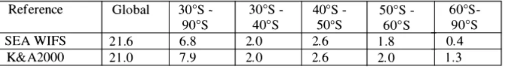
(IPCC, 1996). Southern Ocean emission totals represent approximately one­ third of the global flux, regardless of whether the K&A2000 or Sea WiFS­ derived OMS data base is used as input in the model. Latitudinal distributions based on the two oceanic OMS data bases are similar from 30° to 60°S, but differ markedly south of 60°S.

Table 3. Latitudinal distribution of DMS emissions (TgS yf1) as produced by the LMD-ZT model. SEA WIFS and K&A2000 respectively refer to the simulations that u sed the oceanic DMS concentration maps derived from SeaWiFS data and from the data base of Kettle and Andreae (2000).

Reference Global 30°S - 30°S - 40°S - 50°S - 60°S -90°S 40°S 500S 60°S 90°S S EA WIFS 2 1 .6 6.8 2.0 2.6 1 .8 0.4 K&A2000 2 1 .0 7.9 2.0 2.6 2.0 1 .3

3.3.2. Seasonal variations of DMS emissions

Table 4 presents the primary statistics of monthly OMS emissions in the Southern Ocean. The simulation based on SeaWiFS-derived oceanic OMS concentrations displays a seasonality about 13 times less pronounced than the simulation based on K&A2000. Winter and summer OMS emission t1uxes calculated with the SeaWiFS-derived OMS concentrations are approximately equal, whereas the summer emission flux is markedly higher than winter emission flux when K&A2000 OMS concentrations are used.

Table 4. Minimum, maximum, mean and standard deviation (SD) (in TgS yr·') of monthl y DMS emissions in the southern ocean, between October 1 997 and September 1 998 as produced by the LMD- ZT model, using oceanic DMS concentrations derived from SeaWiFS data and from the data base of Kettle and Andreae (2000).

reference Minimum Maximum Mean S D SEAWIFS 5 .9 7 .2 6.8 0.4 K&A2000 2.4 1 6. 1 7 .9 5 .4

3.3.3. Atmospheric concentrations of sulphur compounds

Figure 8 compares time series of observed and simulated atmospheric concentrations of OMS and non-sea salt sulphate (nss-sulphate) at Amsterdam Island (77°30'E, 37°50'S), Halley (26°l9'W, 75°35'S, Antarctica), and Dumont d'Urville (DDU, 140°l'E, 66°40'S, Antarctica). It should not be forgotten that model predictions are representative of the entire area within a given grid cell, whereas observations are at a very specific point. Also, the predicted values of both gas phase OMS and nss-sulphate depend strongly on the chemical mechanism and other sulphur (anthropogenic, volcanic, etc.) sources used in LMD-ZT model, and the

accuracy with which the model simulates vertical mixing and other meteorological processes. Because of its relatively short atmospheric lifetime (about one day in summer), air concentrations of OMS are closely linked to localized oxidant fields, meteorological mixing processes, and emissions, whereas nss-sulphate, an end product of many atmospheric sulphur oxidation reactions, is likely to have been transported over long distances. Long-term surface measurements of sulphur compounds in the mid- and high- southern latitudes usually display a well marked seasonality, with a summer maximum and a winter minimum (e.g. Sciare et al., 2000; Minikin et al., 1998). This behaviour is captured by the model, as shown in Figure 8. OMS 600. Amsterdam L 400 300. 400. Q 0 200. 100. 0 N 0 J F � A � J J A S 240. Nes sulfate 200. _{Amsterdam r. SQ.} 160. _1\ \ _' I \ _{' '} 120. I _{,, '}

�

40 ao. _' ' 40. ,_ ' 0. 0. 0 N D J F 1.1 A M J J " s OMS Halley 0 N D J F � A M J J A S Nss sulfate ' _Halley . , ., ' ' ' ' I J J '() I 0 N D J F � A 1.1 J J It s 500. �00. 300. ao . 40. 0. 0 0 9-� , 01 I R l '.o l DMS DDU Nse sulfate DDU

�

0 ' --0 �� D J F II It �� J J A S

Figure 8. Seasonal variations in observed and model-predicted atmospheric surface DMS and nss-sulphate (pptv) at Amsterdam Island, Halley and Dumont d'Urville. Solid l ines and dashed lines symbol i ze respectivel y model results using SeaWiFS -derived and K&A2000 oceanic DMS concentrations. Observations are drawn from Sciare et al . (2000) (Amsterdam Island), Mini kin et al . ( 1 998) (Halley) and Jourdain and Legrand (200 I) (Dumont d'Urville).

Figure 8 also indicates that there are substantial differences between observed and simulated atmospheric OMS concentrations (up to factors of -5), regardless of whether K&A2000 or SeaWiFS-derived oceanic OMS

estimates are used. The SeaWiFS-derived DMS simulation produces atmospheric DMS levels at Amsterdam Island that are too high in austral winter and too low in austral summer relative to observations, while at Dumont d'Urville the simulations underestimate DMS and nss-sulphate during the austral summer. Conversely, at Halley simulations using the SeaWiFS-derived and K&A2000 DMS data bases both capture the seasonality of atmospheric nss-sulphate, although the observed nss-sulphate maximum of February occurs in January in both simulations.

Closer agreement between observed and simulated nss-sulphate occurs at Halley when the SeaWiFS-derived oceanic DMS data base is used. Substantial differences between observed and simulated atmospheric DMS concentrations have been noted in other works (e.g., Chin et al., 1996; Barth et al., 2000; Easter et al., 2002), and reflect the difficulties in accurately simulating localized wind fields, mixing and boundary layer phenomena, oxidant fields, and chemical processes in the as yet less-than-fully­ understood atmospheric DMS reaction sequence, all of which influence the gas phase DMS concentrations predicted by any atmospheric general circulation model. Because of these modelling uncertainties, and the limited temporal period of comparison, it is not feasible for us to make any generalizations about which oceanic DMS concentrations data base (K&A2000 or SeaWiFS-derived) is 'better' to use. We note, however, that the use of K&A2000 apparently leads to more realistic atmospheric concentrations of DMS at Amsterdam Island. SeaWiFS-derived DMS concentrations, however, offer the opportunity to document the interannual variations of the marine source of DMS.

The SeaWiFS-derived oceanic DMS data also raise interesting questions for future research efforts. As noted previously, there is a lack of strong seasonality in SeaWiFS images of oceanic chlorophyll concentrations in the vicinity of Amsterdam Island (and thus the SeaWiFS-derived oceanic DMS levels), yet observed atmospheric DMS levels demonstrate a strong seasonality. Do oceanic DMS levels in this region show seasonality, or not? At Amsterdam Island, seawater DMS concentrations varied by a factor of 3.6 between winter and summer with mean concentrations of 0.4 and 1.4 nM, respectively (Nguyen et al., 1990). The maximum DMS concentration was 2 nM in December 1987. Mean DMS fluxes were in the range 1.3-3 11mol m-2 d-1, respectively, so only roughly twice higher in summer than in winter. These results contrast with the more recent data of Sciare et al. (1999). Indeed, the mean concentration and the mean flux of DMS in

December 1997 were 9. 1 nM and 16.4 f.lmol m-2 d-1, respectively. The seawater DMS samples, however, were not collected in the vicinity of Amsterdam Island but in the latitude band 32-38°S about 2000 km to the west of Amsterdam Island. Although fluxes in the range 13-16 f.tmol m-2 d-1 appear to be consistent with long-term observations of summer atmospheric concentrations of DMS and rainwater concentrations of sulphate and methanesulphonate (Sciare et al., 1999), there is no evidence from seawater samples that DMS fluxes in summer closer to Amsterdam Island are indeed in such a range. If not, are atmospheric DMS variations due to localized seasonal differences in atmospheric oxidant fields and mixing processes, or to oceanic processes? For example, the flux of DMS from the ocean to atmosphere may be greater in winter than in summer because of stronger winter winds. If the removal of DMS by ventilation dominates other removal processes in winter, one can expect a feedback on winter sea surface DMS concentrations provided that DMS production from phytoplankton remains unchanged. Also, seasonal changes in phytoplankton speciation or changes in various DMSP and DMS turnover rates may be stronger in the subtropical Indian Ocean than elsewhere. There is currently very little information on the biogeochemistry of oceanic DMS in the area, and more work is clearly needed here and in improving the simulated behaviour of DMS in atmospheric models.

4.

SUMMARY

Oceanic DMS concentration maps can be derived from SeaWiFS satellite data. DMS spatial variability is better captured with this approach relative to earlier works, although there appears to be a tendency to overestimate oceanic wintertime DMS in the mid-latitudes of the southern hemisphere. This tendency occurs because chlorophyll levels, used in deriving the DMS concentrations, remain high in winter at these latitudes. A baseline oceanic DMS level of 1. 1 nM is attained with this technique. With these limitations in mind, nevertheless, we believe that the use of SeaWiFS-derived data should be continued to provide information on the interannual variability and potential climate effects on oceanic DMS.

The gridded SeaWiFS-derived oceanic DMS database can be used as input to three dimensional global atmospheric models. When coupled with parameterizations of the air-sea mass transfer coefficient, estimates of the

flux of DMS from the ocean to the atmosphere can be obtained via model simulations. Using the three-dimensional atmospheric General Circulation Model of the Laboratoire de Meteorologie Dynamique, model-time-step wind speeds, an atmospheric-stability-dependent parameterization of the mass transfer coefficient, and the SeaWiFS-derived oceanic DMS distributions, we estimate an annual southern ocean DMS emission of 6. 8 Tg S y( 1 • This value represents approximately one-third of the annual global

DMS marine emission, and underscores the importance of this region as a source of natural sulphur emissions.

5. REFERENCES

Anderson. T. R., S. A. Spall, A. Yool. P. Cipollini. P. G. Challenor, and M. J. R. Fasham. Global fields of sea surface dimethylsulfide predicted from chlorophyll, nutrients and light, J. Mar. Syst. . 30, 1 -20, 200 I .

Aranami, K. , S. Watanabe, S. T'unogai, M. Hayashi, K. Furuya, and T. Nagata, Biogeochemical variation in dimethylsulfide, phytoplankton pigments and heterotrophic bacterial production in the Subarctic North Pacific during summer, J. Oceanogr. , 57. 315-322,

200 1 .

Archer, S.D. , F.J. Gilbert, P.D. Nightingale. M. V . Zubkov. A.H. Taylor, G.C. Smith. and P.H. Burkill, Transformation of dimethylsulfoniopropionate to dimethylsulfide during summer in the North Sea with an examination of key processes via a modelling approach. Deep-Sea Res. II, 49, 3067-3101, 2002 .

Aumont, 0., S. Belviso. and P. Monfray, Dimethylsulfoniopropionate (DMSP) and dimethylsulfide (DMS) sea surface distributions simulated from a global 3-D ocean carbon cycle model. J. Geophys. Res., 1 07, C4. 10.102911999 JC000 1 1 1, 2002.

Barrie, L.. Y. Yi. W.R. Leaitch, U. Lohmann, P. Kasibhatla, G.-J. Roelofs. J. Wilson, F. McGovern, C. Benkovitz. M.A. Meliere, K. Law, J. Prospera, M. Kritz, D. Bergmann, C. Bridgeman. M. Chin, J. Christensen, R. Easter, J. Feichter, C. Land, A. Jeuken, E. Kjellstrom, D. Koch, and P. Rasche! al. , A comparison of large scale atmospheric sulphate aerosol models (COSAM): Overview and highlights, Tell us, 5 3B, 625-645, 200 1 .

Barth, M. C., P. J. Rasch, J. T. Kiehl, C. M. Benkovitz and S. E. Schwartz, Sulfur chemistry in the National Center for Atmospheric Research Community Climate Model: Description, evaluation, features, and sensitivity to aqueous chemistry, J. Geophys. Res., 105, 1387-1415, 2000.

Bates. T. S .. 1. D. Cline, R. H. Gammon, and S. R. Kelly-Hansen, Regional and seasonal variations in the flux of oceanic dimethylsulfide to the atmosphere, J. Geophys. Res. , 92. 2930-2938, 1 987.

B ates, T. S . , B. K. Lamb, A. Guenther, J. Dignon, and R. E. Stoiber, Sulfur emissions from natural sources, J. Atmos . Chern. , 14, 3 1 5-337, 1 992.

B ates, T. S., V.N. Kapustin, P.K. Quinn, D.S. Covert, D.J. Coffman, C. Mari, P.A. Durkee, W.J. DeBrutn, and E. Satzman, Processes controlling the distribution of aerosol particles in the lower marine boundary layer during the First Aerosol Characterization Experiment (ACE­

I), J. Geophys. Res. , 1 03 , 1 6,369- 1 6,383, 1 998.

Belviso, S., R. Morrow, and N. Mihalopoulos, An Atlantic meridional transect of surface water dimethylsulfide concentrations with 1 0- 1 5 km horizontal resolution and close examination of ocean circulation. J. Geophys. Res. 1 05 , 1 4,423 - 1 4,43 1 , 2000.

B enkovitz, C. M., C. M. Berkowitz, R. C. Easter, S . Nemesure, R. Wagener, and S. E. Schwartz, Sulfate over the North Atlantic and adjacent continental regions : Evaluation for October and November 1 986 using a three-dimensional model driven by observation-derived meteorology, J. Geophys. Res. , 99, 20,725 -20,756, 1 994 .

Boucher, 0., M. Pham, and C. Venkataraman, Simulation of the atmospheric sulfur cycle in the Laboratoire de Meteorologie D ynamique General Circulation Model. Model description, model evaluation and global and European budgets, Note scientifique 23 de I'Institut Pierre Simon Laplace, Paris, France, 2002.

Chapman, E . G. , R. C. Easter, X . Bian, and S . J. Ghan, The influence of wind speed averaging on estimates dimethylsulfide emission fluxes, J. Geophys. Res . , 1 07, 1 0 . 1 029, doi: 200 1 JDOO I 564, 2002.

Chin, M., D . J. Jacob, G. M. Gardner, M. S . Foreman-Fowler, and P. A. Spiro, A global three­ dimensional model of tropospheric sulfate, J. Geoph ys. Res . , 1 0 1 , 1 8667- 1 8690, 1 996. Chin, M., R. B. Rood, S . -J. Lin, J. -F. Muller, and A. M . Thompson, Atmospheric sulfur cycle simulated in the global model GOCART: Model description and global properties, J. Geophys. Res. , I 05, 24,67 1 -24,687, 2000.

Chuang, C . , J. E. Penner, K. E. Taylor, A. S. Grossman, and J. W. Walton, An assessment of the radiative effects of anthropogenic sulfate, J. Geophys. Res., I 02, 376 1 -3778, 1 997. Claustre, H., The trophic status of various oceanic provinces as revealed by phytoplankton. pigment signatures, Limnol. Oceanogr., 39, 1 206- 1 2 1 0, 1 994.

Cosme, E., C. Genthon, P. Martinerie, 0. Boucher and M. Pham, The sulfur cycle at high­ southern latitudes in the LMD-ZT General Circulation Model, J. Geophys . Res., I 07, 4690,

1 0.1 029/2002JD002 1 49, 2002.

Easter, R. C., S. J. Ghan, Y. Zhang, R. D. Saylor, E.G. Chapman. N. S. Laulainen, H. Abdui­ Razzak, L. R. Leung, X. B ian and R. A. Zaveri, MIRAGE: Model description and evaluation of aerosols and trace gases, submitted for pub lication in J. Geophys. Res., 2002.

Feichter, J., E. Kjellstrom, H. Rodhe, F. Dentener, J. Lelieveld, and G-J. Roelofs, Atmos. Environ., 30. 1 693- 1 707, 1996.

Frost, T. and R. C . Upstill-Goddard, Air-sea gas exchange into the millennium: Progress and uncertainties, in Oceanography and Marine Biology: an Annual Review, 37, 1 -45, 1 999. Genthon, C., G. Krinner, and E. Cosme. Free and l aterally-nudged antarctic climate of an atmospheric general circul ation model, Mon. Wea. Rev. , 1 30, 1 60 1 - 1 6 1 6, 2002.

Ghan, S., R. Easter, E. Chapman, H. Abdui-Razzak, Y. Zhang, R. Leung, N. Laulainen, R. Saylor and R. Zaveri, A physically based estimate of radiative forcing by anthropogenic sulfate aerosol, J. Geophys. Res. , 1 06, 5279-5293 , 200 1 a.

Ghan, S . , N. Laulainen, R. Easter, R. Wagener, S . Nemesure, E. Chapman, Y. Zhang and R. Leung, Evaluation of aerosol direct radiative forcing in MIRAGE, J. Geophys. Res. , I 06, 5295-53 1 6, 200 l b .

Hansson, M . E . and E. S . Saltzman, The first Greenland ice core record o f methanesulfonate and sulfate over a full glacial cycle, Geophys. Res. Lett. , 20, 1 1 63 - 1 1 66, 1 993.

IPCC, Climate Change, 1 995 : The science of climate change, edited by J. T. Houghton, L. G. Meira Filho, J. Bruce, H. Lee, B . A. Callander, E. Haites, N. Harris and K. Maskell, Canbridge University Press, 1 996.

Jones, A., D. L. Roberts, M. J. Woodage, and C . E. Johnson, Indirect sulphate aerosol forcing in a climate model with an interactive sulphur cycle, J. Geophys. Res. , 1 06, 20.293-20, 3 1 0, 200 1 .

Jourdain B. and M. Legrand, Seasonal vanatwns of atmospheric dimethylsulfide, dimethylsulfoxide. sulfur dioxyde, methanesulfonate and non-sea-salt sulfate aerosols at Dumont d'Urville (coastal Antarctica, December 1 998-July 1 999). J . Geophys. Res. , 1 06, 1 4,39 1 - 1 4,407, 200 1 .

Kettle, A . J., M.O. Andreae, D . Amouroux, T.W. Andreae, T. S . Bates, H . Berresheim, H . B ingemer, R . Boniforti, M . A.J. Curran, G.R. DuTullio, G . Helas, C . B . Jones, M.D. Keller, R.P. Kiene, C. Leek, M . Levasseur, M. Maspero, P. Matrai, A.R. McTaggart, N. Mihalopoulos, B . C . Nguyen, A. Novo, J.P. Putaud, S. Rapsomanikis, G. Roberts, S . Schebeke, R. Simo, R. Staubes, S . Turner, ans G . Uher, A global database o f sea surface dimethylsulfide (DMS) measurements and a procedure to predict sea surface DMS as a function of latitude, longitude, and month, Global B iogeochem. Cycles, 1 3 , 399-444, 1 999. Kettle, A.J. and M . 0. Andreae, Flux of dimethylsulfide from the oceans: A comparison of updated data sets and flux models, J. Geophys. Res . , 1 05, 26,793-23 ,808, 2000.

Kiene, R. P . , L. J. Linn, J. A. Burton, New and important roles for DMSP in marine microbial communities, J. Sea Res. , 43, 209-224, 2000.

Koch, D., D. Jacob, I. Tegen, D. Rind, and M. Chin, Tropospheric sulfur simulation and sulfate direct radiative forcing in the Goddard Institute for Space Studies general circulation model, J. Geophys. Res . , 1 04, 23,799-23 , 822, 1 999.

Krinner, G., C. Genthon, Z.X. Li, and P. Le Van, Studies of the Antarctic climate with a stretched-grid general circulation model, J. Geophys. Res. , 1 02, 1 3 ,73 1 - 1 3 ,745 , 1 997. Legrand, M., C . Feniet-Saigne, E. S . Saltzman, C. Germain, N. I. Barkov, and V. N. Petrov, Ice-core record of oceanic emissions of dimethylsulfide during the last climatic cycle, Nature, 350, 1 44- 1 46, 1 99 1 .

Liss, P . S . and L . Merlivat, Air-sea gas exchange rates : Introduction and synthesis, in The Role of Air-Sea Exchange in Geochemical Cycling, edited by P. B . Menard, pp. 1 1 3- 1 27 . D. Reidel, Norwell, Mass., 1 986.

Lohmann, U . , K. von Salzen, N. McFarlane, H . G. Leighton, and J. Feichter, Tropospheric sulfur cycle in the Canadian general circulation model, J. Geophys. Res. , 1 04, 26,833-26,858, 1 999.

Minikin, A., M . Legrand, J. Hall, D. Wagenbach, C . Kleefeld, E. Wolf, E. C. Pasteur, and F. Ducroz. Sulfur-containing species (sulfate and methanesulfonate) in coastal Antarctic aerosol and precipitation, J. Geophys. Res., 103, 1 0,97 5 - 1 0,990, 1 998.

Nightingale, P. D . , G. Malin, C . S . Law, A. J. Watson, P . S . Liss, M. I. Liddicoat, J. Boutin and R. C. Upstill-Goddard, In situ evaluation of air-sea gas exchange parameterizations using novel conservative and volatile tracers, Glob. Biogeochem. Cycles, 1 4, 373-387, 2000. Nguyen, B . C . , N. Mihalopoulos, and S. Belviso, Seasonal variation of atmospheric dimethylsulfide at Amsterdam Island in the S outhern Indian Ocean, J. Atmos . Chern. , 1 1 ,

1 23- 1 4 1 , 1 990.

Pham, M., J.-F. Muller, G. Brasseur, C. Granier, and G. Megie, A three-dimensional study of the tropospheric sulfur cycle, J. Geophys. Res. , 1 00, 26,06 1 -26,092, 1 995.

Roeckner, E . , L. Bengtsson, J. Feichter, J. Lelieveld and H. Rodhe, Transient climate change simulations with a coupled Atmosphere-Ocean GCM including the tropospheric sulfur cycle, J. Clim., 1 2, 3004-3032, 1 999.

Sciare, J., N . Mihalopoulos, and B . C. Nguyen, Summerti me seawater concentrations of dimethylsulfide in the Western Indian Ocean: reconciliation of fluxes and spatial variability with long-term atmospheric observations, J. Atmos. Chern. , 32, 357-373, 1 999.

Sci are, J . , M. Kanakidou, and N. Mihalopoulos, Diurnal and seasonal variation of atmospheric dimethylsulfoxide (DMSO) at Amsterdam Island in the southern Indian Ocean . J. Geophys. Res . , 1 05 , 1 7,257- 1 7 ,265 , 2000.

Spiro, P. A . , D. J. Jacob, J. A. Logan, Global inventory of sulfur emissions with l 0X l 0 resolution. J . Geophys . Res . , 97, 6023 -6036, 1 992.

Zubkov. M. V., B. M. Fuchs. S . D. Archer, R. P. Kiene, R. Amann, and P. H. Burkill, Linking the composition of bacterioplankton to rapid turnover of dissolved dimethylsulfonio­ propionate in an algal bloom in the North Sea. Environ. Microbial . , 3 , 304-3 1 1 , 200 1 .