HAL Id: hal-03191256
https://hal.archives-ouvertes.fr/hal-03191256
Submitted on 7 Apr 2021HAL is a multi-disciplinary open access archive for the deposit and dissemination of sci-entific research documents, whether they are pub-lished or not. The documents may come from teaching and research institutions in France or abroad, or from public or private research centers.
L’archive ouverte pluridisciplinaire HAL, est destinée au dépôt et à la diffusion de documents scientifiques de niveau recherche, publiés ou non, émanant des établissements d’enseignement et de recherche français ou étrangers, des laboratoires publics ou privés.
To cite this version:
Michiel Postema, Spiros Kotopoulis, Klaus-Vitold Jenderka. Physical principles of medical ultrasound. Christoph F. Dietrich. EFSUMB Course Book 2nd Edition, pp.1-23, 2019, �10.37713/ECB01�. �hal-03191256�
Physical principles of medical ultrasound
1 2
Michiel Postema1,2,3, Spiros Kotopoulis4, Klaus-Vitold Jenderka5 3
4
1 School of Electrical and Information Engineering, University of the Witwatersrand, 5
South Africa; 6
2 Inserm Research Unit U930: Imaging and Brain, Université François-Rabelais de 7
Tours, France; 8
3 LE STUDIUM Loire Valley Institute for Advanced Studies, Orléans, France; 9
4 Department of Gastroenterology, Haukeland University Hospital, Bergen, Norway; 10
5 Department of Engineering and Physics, Merseburg University of Applied 11
Sciences, Merseburg, Germany. 12
13
Sound and ultrasound
14
Acoustics is the scientific field that studies sound. Sound is a form of mechanical 15
periodic molecular displacement (vibration) of matter. The time it takes for a vibration 16
cycle to complete is called a period. The number of vibration cycles that occur during 17
a set time is referred to as the frequency. The frequency f of a vibration is the inverse 18 of its period T: 19 20 Eq. 1 21
Sound with frequencies below 20 cycles per second, i.e., below 20 Hz, is called 22
infrasound. Although infrasound is too low to be heard by human beings, it can be 23
perceived (felt). 24
The audible range is defined by frequencies between 20 Hz and 20,000 Hz (20 kHz). 25
This range has been defined by the average hearing of healthy 18-years-old men. 26
Frequencies higher than 20 kHz are referred to as ultrasound. 27
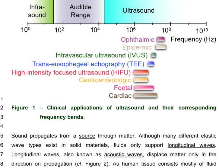
Figure 1 shows some clinical application of ultrasonics and their respective frequency 28
bands. 29
31
Figure 1 – Clinical applications of ultrasound and their corresponding 32
frequency bands. 33
34
Sound propagates from a source through matter. Although many different elastic 35
wave types exist in solid materials, fluids only support longitudinal waves. 36
Longitudinal waves, also known as acoustic waves, displace matter only in the 37
direction on propagation (cf. Figure 2). As human tissue consists mostly of fluid 38
materials, primarily longitudinal waves are generated and observed in the field of 39
medical ultrasonics. 40
42
Figure 2 - Schematic representation of the axial displacement of matter by a 43
longitudinal sound wave. 44
45
The highest displacement in a sound wave is called the displacement amplitude. 46
Generally, the matter displacement in space and time by a low-amplitude sound 47
wave has the form 48
49
Eq. 2 50
where 𝑢! is the displacement amplitude and 𝜆 is the wavelength of the sound (cf. 51
Figure 2). 52
53
Notice the minus between #" and $% in (2): obviously, the wave at given time farther 54
from the source is equal to the wave at earlier time closer to the source. Taking only 55
one dimension into account, the compressive and extensive displacements are 56
related to local pressure changes by the equation of motion from which the wave 57
equation is derived (cf. Appendix, Eq. A 1 – A 3). 58
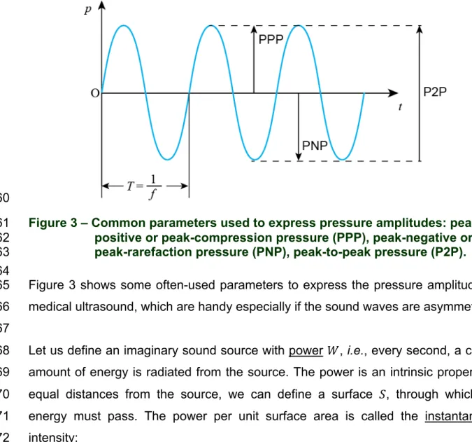
59
60
Figure 3 – Common parameters used to express pressure amplitudes: peak-61
positive or peak-compression pressure (PPP), peak-negative or 62
peak-rarefaction pressure (PNP), peak-to-peak pressure (P2P). 63
64
Figure 3 shows some often-used parameters to express the pressure amplitudes of 65
medical ultrasound, which are handy especially if the sound waves are asymmetric. 66
67
Let us define an imaginary sound source with power 𝑊, i.e., every second, a certain 68
amount of energy is radiated from the source. The power is an intrinsic property. At 69
equal distances from the source, we can define a surface 𝑆, through which this 70
energy must pass. The power per unit surface area is called the instantaneous 71
intensity: 72
Eq. 3 73
The averaged derived intensity of a harmonic sound wave at a point in a sound field 74 is: 75 76 Eq. 4 77
where 𝑝& is the pressure amplitude, 𝑐 is the speed of sound in the medium, and 𝜌 is 78
the density of the medium. Thus, for a point source, the surface through which the 79
energy must pass is a sphere of radius 𝑟 (cf. Figure 4) and a surface area 𝑆 = 4𝜋𝑟'.
80
Consequently, for a point source, the intensity is inversely proportional to the 81
distance to the source squared, and the acoustic pressure is inversely proportional to 82
the distance itself. This acoustic pressure decay with distance is called geometric 83
damping. 84
85
86
Figure 4 – Radiated field through a spherical surface S at a distance r from a 87
point source with power W. 88
89
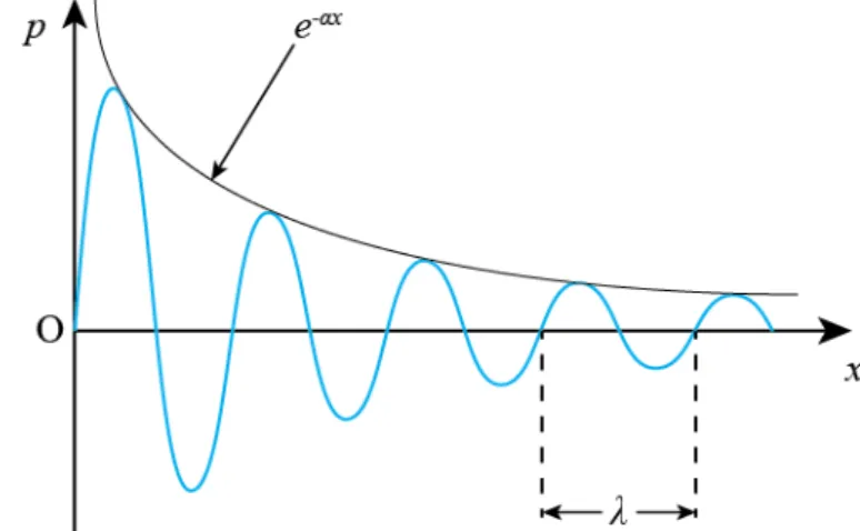
Thermal and viscous material properties are other causes of damping of the acoustic 90
wave (cf. Figure 5). Damping coefficients are frequency-dependent. In human tissue, 91
the damping coefficient is proportional to the frequency to a power between 1.0 and 92
1.4. Thus, the higher the frequency, the lower the penetration depth of the sound. 93
94
95
Figure 5 – Damped wave with wavelength 𝝀 and damping coefficient 𝜶. 96
97
The amplitude of a received acoustic signal is generally expressed in decibels 98
relative to a reference pressure: 99
Eq. 5 101
where SPL is the sound pressure level in decibels. Decibels are always rounded to 102
whole numbers. Table 1 gives some typical values for pressure changes and their 103
respective level in decibels. 104 105 SPL [dB] Multiplication -20 0 .10× -12 0 .25× -6 0 .50× 0 1 × 6 2 × 12 4 × 20 10 × 40 100 × 60 1,000 × 80 100,000 ×
Table 1 – Sound pressure levels and their corresponding multipliers. 106
107
Most acoustic waves propagate unhindered through the human body. A small 108
proportion is specularly reflected on tissue transitions. The amount of reflected sound 109
at such a boundary is dependent of the acoustic impedances on both sides of the 110
boundary. The acoustic impedance Z of a medium is defined by 111
112
Eq. 6 113
where 𝑐( and 𝜌( are the speed and the density, respectively, of medium 𝑖. Reflection 114
and transmission coefficients are used to predict reflections from boundaries. 115
In most organs, tissues have rather small acoustic impedance differences. The 116
boundaries consist of cells with sizes much smaller than the wavelength of the 117
ultrasound used for imaging. The signals travelling back to the sound source from 118
tissue transitions are actually caused by scattering. Given the long wavelengths of 119
the ultrasound, cells can be considered point scatterers. The backscattering from 120
point scatterers is proportional to the number of scatterers per volumetric unit 121
(scattering density), proportional to the square of the combined compressibility and 122
density differences of the scatterers, inversely proportional to the fourth power of the 123
wavelength and therefore proportional to the fourth power of the frequency, and 124
proportional to the sixth power of the radii of the point scatterers. For larger 125
scatterers, such as collagens or veins, the scattering behaviour is different from the 126
so-called Rayleigh scattering from point scatterers. The backscattering properties 127
have been quantified for many structures of millimetre-size in organs. Using these 128
quantifications of backscattered signal, abnormalities can be traced. As an example, 129
fatty liver cirrhosis can be traced from the change in scattering from enlarged mean 130
distances between lobular structures. 131
132
Moving scatterers such as blood cells create a shift in the ultrasound signal. This so-133
called Doppler shift can be approximated by 134
135
Eq. 7 136
where 𝜃 is the angle between the ultrasound beam and the streaming direction 137
(positive axis) and 𝑣 is the magnitude of the streaming velocity (cf. Figure 6). 138
139
Figure 6 – Lateral velocity as a function of Doppler shift at four different 141
transmitting frequencies. 142
143
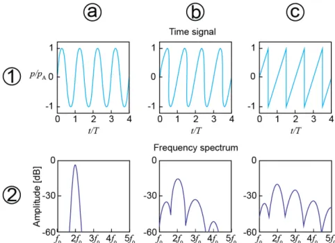
Changes in the frequency of the signal are also caused by nonlinear propagation 144
through tissue and by the presence of ultrasound contrast agents. Nonlinear 145
propagation is caused by the fact that the speed of sound in compressed tissue is 146
slightly higher than in extended tissue. Therefore, the peaks of ultrasound waves 147
travel faster than the troughs. The waves are distorted farther away from the source, 148
until only saw-tooth shapes remain. Figure 7 shows some waveforms at different 149
distances from the source, and their frequency content. 150
151
152
Figure 7 – Waveforms at different distances from the source, and their 153
respective frequency spectra. 154
155
Blood cells are poor scatterers in diagnostic ultrasound. Because perfusion imaging 156
is often desired in clinical diagnosis, ultrasound contrast agents have been injected to 157
enhance the scattering from blood. Ultrasound contrast agents consist of 158
microscopically small perfluorocarbon gas bubbles encapsulated by elastic (most 159
commonly phospholipid) shells. These microbubbles oscillate linearly and nonlinearly 160
in sound fields, radiating a detectable acoustic signal. Several detection strategies 161
exist to reveal the presence of microbubbles and therefore blood (cf. Figure 8). 162
Recently, the peculiar behaviour of microbubbles under specific acoustic conditions 163
close to living cells has led to research into therapeutic applications of microbubbles 164
whose shells have been modified to contain drugs or genes. Ultrasound-guided drug 165
delivery might be possible using regular clinical ultrasound equipment. 166
167
168
Figure 8 – Two detection strategies for the presence of microbubbles. 169
170
Transducers
171
Ultrasound transducers convert electrical signal to pressure waves and vice versa. 172
With therapeutic devices, such as those used for physiotherapy or ultrasound-173
mediated surgery, only the transmit capability is used, whereas diagnostic devices 174
both transmit and receive. In all cases, transducers contain piezoelectric elements to 175
generate ultrasound or convert ultrasound into an electrical signal. 176
When strain is applied, the electric charges in the elements are redistributed, 177
therefore generating an electrical impulse. Inversely, when an electrical impulse is 178
applied, it changes the geometry of the piezoelectric material. This is true for all 179
piezoelectric materials. 180
181
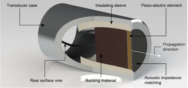
Apart from one or more piezoelectric elements with electrodes attached to both 182
sides, ultrasound transducers consist of a backing behind the element, and one or 183
more matching layers in front of the element (cf. Figure 9). 184
186
Figure 9 – Components of a single-element transducer. 187
188
The thickness of the element determines its resonance frequency: its natural 189
oscillation frequency. Without backing present, the element can oscillate with 190
maximum amplitude, i.e., extend and contract, at this frequency. The backing 191
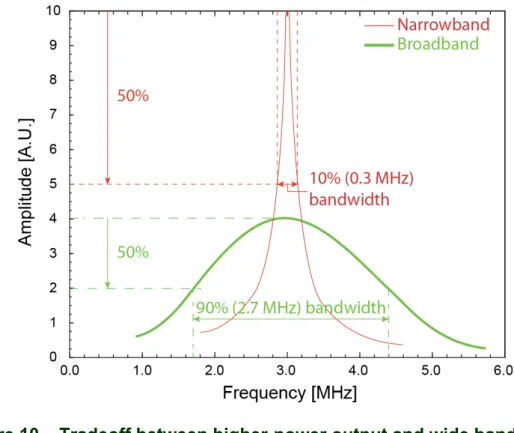
material determines the bandwidth of the transducers. The bandwidth is the 192
frequency band at which a transducer generates and receives sound (cf. Figure 10). 193
The choice of backing material is critical for the performance of the transducer. The 194
matching layer forms a near-lossless transition between the element and the 195
medium. 196
198
Figure 10 – Tradeoff between higher-power output and wide bandwidth. 199
200
A transmitting transducer creates a sound field. Close to the transducer surface, 201
interference causes local pressure variations (cf. Figure 11). The width of this so-202
called near field is roughly equal to the diameter of the transducer. Its length is given 203
by 204
Eq. 8 205
where 𝐷 is the transducer diameter and 𝑁 is the near-field length. In the far field, the 206
sound field propagates with an opening angle 2𝛾: 207
208
Eq. 9
210
Figure 11 – Profiles of a sound field: (a) schematic; (b) 2D; (c) axial: (d) lateral. 211
212
The axial plane separating near field from far field is the natural focus of a 213
transducer. A sound field can be further geometrically focussed by adding an 214
acoustic lens to the transducer surface. 215
In clinical ultrasound machines, multi-element transducers are used (cf. Figure 12). 217
These consist of arrays of transducer elements lined up in the lateral direction, which 218
can be individually controlled, allowing for variable beam focussing (cf. Figure 12). 219
Such so-called phased arrays exist in numerous layouts, including curvilinear, 1.5D, 220
and 2D variations (cf. Figure 13). 221
222
223
Figure 12 – Phased-array probes with variable focusing. 224
225
226
Figure 13 – Phased arrays and their beam profiles: (a) 1D; (b) curvilinear; (c) 227
2D. 228
Imaging
229
Unlike a continuous sound wave, ultrasound for diagnostic imaging is transmitted as 230
a pulse sequence (cf. Figure 14). After transmission of a pulse with a certain centre 231
frequency, backscattered signal from tissue is received until the next pulse is 232
transmitted. The pulse repetition frequency (PRF) is the number of pulses per time 233
unit. The duty cycle is the percentage of transmission time, equal to the pulse length 234
times the PRF. The theoretical maximum distance of imaging is 235
236
Eq. 10
Beware that the local speed of sound varies for different tissues. Therefore, 238
ultrasound images built from the two-way travel times recorded are not converted to 239
actual depth. The most commonly used mean speed of sound for quasi-depth 240
conversion is 1540 m/s, which is the mean speed of sound in soft tissue (cf. Table 2). 241
As this is just a chosen value, great care should be taken when drawing conclusions 242
from quantitative spatial measurements using ultrasonic imaging. 243 244 Material/tissue c [m/s] Air 330 Silicon oil 980 Water 1490 Blood 1570 Fat 1460 Muscle 1580 Bone 3500
Mean in soft tissue 1540
Table 2 – Speed of sound for different biomaterials. 245
246
247
Figure 14 – Pulsed transmit signal, with a centre frequency fc, pulse length PL,
248
pulse repetition time PRT, pulse repetition frequency PRF. The duty 249
cycle of this signal is 25%. 250
252
Figure 15 – Principle of B-mode imaging. 253
254
Figure 15 shows how a single beam is creating a line in an ultrasound image. If only 255
the signal amplitude (“A”) is considered, the imaging mode is called A-mode, 256
whereas the amplitudes are represented by spots of brightness (“B”) are more than 257
one dimension, we speak of mode. Table 2 shows some typical applications of B-258
mode and the frequencies of choice. B-mode is the default clinical ultrasonic imaging 259
method. B-mode is often combined with Doppler methods to track moving targets. 260
Using probes with mechanically moving transducers or 2D arrays, 3D B-mode scans 261
can be recorded. 262
263 264
Frequency [MHz] Penetration depth [cm] Target organ 2-3 30 Deep abdomen 4-5 20 Adult heart 12-15 3 Mammae, Thyroid, Endosonography 20-50 1 Eye
Table 3 – Some B-mode applications and their fundamental imaging 265
frequencies. 266
267
268
Figure 16 – M-mode imaging principle. 269
Displaying the received signal along one beam in motion (“M”), i.e., as a function of 270
time is called M-mode. The high time resolution allows for detailed study of 271
periodically moving objects, such as the heart or a blood vessel (cf. Figure 16). 272
273
Resolution is the minimum distance between two points for them to be discriminated 274
as separate points. The axial resolution is equal to the speed of sound divided 275
through by twice the bandwidth. Hence, the wider the bandwidth (or the shorter the 276
pulse length) is, the smaller (better) the axial resolution is. The lateral resolution is 277
proportional to the wavelength of the sound and the transducer focal depth, and 278
inversely proportional to the transducer aperture. 279
280
Safety indices
281
The mechanical index (MI) gives an indication for the mechanical damage of tissue 282
due to inertial cavitation: the ultrasound-induced formation of transient cavities: 283
284
Eq. 11
285
where PNP is the maximum value of the peak-negative pressure anywhere in the 286
ultrasound field (measured in water but corrected for a different attenuation) 287
normalised by 1 MPa and 𝑓) is the centre transmit frequency normalised by 1 MHz.
288
At MI < 0.3, the acoustic amplitude is considered low enough for neonatal scans and 289
pregnant women. At 0.3 < MI < 0.7, there is risk of minor damage to neonatal lung 290
and intestine. At MI > 0.7, there is a theoretical risk of inertial cavitation and a more 291
substantial risk if ultrasound contrast agents are being used. 292
Although the validity of the MI has been disputed, especially if an ultrasound contrast 293
is used, there is currently no alternative available to judge the safety from cavitation-294
related damage in clinical settings. 295
Another, disputed, safety index is the thermal index (TI). It is a rough indicator of the 296
temperature rise in tissue during ultrasound exposure, and defined by the ratio of the 297
transmitted power and the estimated power needed to raise the tissue temperature 298
1oC. It should be noted that the TI does not indicate the actual temperature rise. 299
Based on thermal indices, limitations to ultrasound exposure times have been 300
recommended. 301
Near-future research will have to concentrate on redefining the safety standards. 302
303 304
Further reading
305
[1] Hoskins P, Martin K, Thrush A (Eds). Diagnostic Ultrasound: Physics and 306
Equipment. Cambridge: Cambridge University Press 2010. 307
[2] Millner R, Jenderka K-V. Physik und Technik der Ultraschallanwendung in der 308
Medizin. Studienbrief MPT0015. Kaiserslautern: Technische Universität 309
Kaiserslautern 2010. 310
[3] Postema M. Fundamentals of Medical Ultrasonics. London: Spon Press 2011. 311
[4] Schmitz G. Ultrasound in medical diagnosis. In: Pike R, Sabatier P (Eds). 312
Scattering: Scattering and Inverse Scattering in Pure and Applied Science. 313
London: Academic Press 2002:162-174. 314
315
Appendix
316
The equation of motion is 317
318
Eq. A 1 where 𝜌 is the density of the medium.
319
The linear 1-dimensional wave equation gives the sound pressure as a function of 320
space and time: 321
322
Eq. A 2
The speed of sound 𝑐 = 𝜆𝑓 = 8*+ is a material property of the medium. Here, 𝜅 is the 323
bulk (incompressibility) modulus. Solutions of the wave equation have the form: 324
325
Eq. A 3 where 𝑘 =',% is the wave number and 𝑝& is the pressure amplitude.
326 327