A combined Kalman Filter and Error in Constitutive Relation approach for system identification in structural dynamics.

HAL Id: pastel-00724815

https://pastel.archives-ouvertes.fr/pastel-00724815

HAL is a multi-disciplinary open access archive for the deposit and dissemination of sci-entific research documents, whether they are pub-lished or not. The documents may come from teaching and research institutions in France or abroad, or from public or private research centers.

L’archive ouverte pluridisciplinaire HAL, est destinée au dépôt et à la diffusion de documents scientifiques de niveau recherche, publiés ou non, émanant des établissements d’enseignement et de recherche français ou étrangers, des laboratoires publics ou privés.

A combined Kalman Filter and Error in Constitutive

Relation approach for system identification in structural

dynamics.

Albert Alarcon Cot

To cite this version:

Albert Alarcon Cot. A combined Kalman Filter and Error in Constitutive Relation approach for system identification in structural dynamics.. Mechanics of the structures [physics.class-ph]. Ecole Polytechnique X, 2012. English. �pastel-00724815�

Une approche de l’identification en dynamique des

structures combinant l’erreur en relation de

comportement et le filtrage de Kalman

Th`ese pr´esent´ee pour l’obtention du titre de

DOCTEUR DE L’ ´ECOLE POLYTECHNIQUE Sp´ecialit´e : M´ecanique

par

Albert Alarc´on Cot

Soutenue le 4 juin 2012 devant le jury compos´e de

Pr´esident : Claude Blanz´e Professeur, CNAM, France

Rapporteurs : Laurent Champaney Professeur, ENS-Cachan, France Geert Lombaert Professeur, KU Leuven, Belgique

Examinateur : Andrew W. Smyth Professeur, Columbia University, USA

Directeur : Marc Bonnet Directeur de recherche, CNRS, France

Encadrant : Charles Bodel Ing´enieur de recherche, EDF, France

Laboratoire de M´ecanique des Solides LaMSID ´

`a Carole

a la meva fam´ılia

Acknowledgments

I would like to express my most sincere gratitude to my advisors, Marc Bonnet and Charles Bodel, not only for the quality of their guidance but also for the confidence they offered me from the very beginning and the patience and help they showed all along this period.

I also owe all my gratitude to all the members of my defense committee: Claude Blanz´e for accepting being the committee chairman, Geert Lombaert and Laurent Champaney for their effort in reviewing this dissertation, their questions, comments, and useful feedback on this work. And obviously, a very special thanks to Andrew W. Smyth for having accepted to be part of my defense committee, which honors me, but also for warmly hosting me at Columbia University during a summer internship, where I had the chance to share rich and inspiring interactions with him.

During this work, I spent most of my time at the Mechanics and Acoustics research department of EDF, where I always felt pleased to work. I would therefore like to sincerely thank Laurent Billet, Sebastien Caillaud and Franc¸ois Weackel, not only for having accepted me as a Ph.D student, but also for their permanent trust that made possible new, challenging, projects such as giving me the possibility work at Columbia University or establishing a cooperation with the LMT laboratory of ENS-Cachan.

In the cooperation with the LMT, I had he chance to work with Frederic Ragueneau and the LMT laboratory fellows in the construction of a nontrivial test setup, and I would like to acknowledge them for their invaluable contribution.

Of course, this research wouldn’t had been possible without Mathieu Corus and Jean-Philippe Argaud from EDF R&D, with whom I had discussion of priceless help from both technical and scientific point of view. I cannot forget either the nice experience I had supervising Ma¨ılys Pache during her final-year undergraduate internship. Her commitment and diligence considerably helped me to both improve this work and acquire a deeper insight of the involved techniques.

And, most importantly, I want to thank, warmly, all those who have have been there for all what is not written hereafter: colleagues, new and old friends, and all the people I love. The list will be too long, but let me at least mention a few, starting from the guys from the Laboratoire de M´ecanique des Solides of the ´Ecole Polytechnique, with a special big up to Eva and Nico, whose ability to unconditionally make me laugh goes far beyond expectations. I also truly want to thank all the colleagues from T61 without exception, for their permanent good vibes. And specially “la bande de joyaux connards” with Laurent, Thibaud, Charles, Lise, John ’Blue Eyes’,Nicolas, JC and Emeric, for having shared so many “romantiK“ moments together and inspired me day after day. The moments I spent in NYC will also last

f

as an unforgettable experience and I wish to specially thank Mike, Adrian, and particularly Aude for her contagious energy. I won’t forget to broadly thank all my friends who have continuously been by my side, for their continuous encouragement and interest that helped me carry on, and all those little moments that makes a strong whole. Special thoughts go to Laura, Esteban and Paola without whom anything would be as it is today, so many ”calle treces, haches intercaladas, loquitos-por-ti, peches, penestines, guayavez, vueltas imposibles, vinitos y trasnochadas“ to regret.

For sure, I would also wish to express all my gratitude to my beloved family, from Barcelona to Caen, from the youngest (2!) to the elder (99!) whose unconditional love made this thesis possible.

Finally, and above all, my deepest gratitude and love goes to Carole for her never ending encourage-ment, support, patience and love during all these years.

Abstract

Throughout its industrial activity, and particularly in the field of structural vibrations, French electricity producer EDF faces dimensioning, monitoring and diagnosis problems. Experimental information is often combined with numerical simulations to complete the a priori knowledge of structural behavior needed to address industrial issues. Vibration expertise is thus required in a broad range of fields such as health monitoring, structural modification assessment and boundary conditions identification.

This work aims to find a method to combine experimental and numerical information for model-updating purposes and thus improve their predictive power. More specifically, the problem of structures with evolutionary mechanical properties is addressed. To this end, this thesis proposes a combined use of the Error in Constitutive Relation (ECR) and Kalman filtering (KF) techniques.

In structural dynamics, the ECR is an energy-based approach to solve inverse problems. ECR func-tionals measure the model error by evaluating the difference between kinematically and dynamically admissible fields using an energy norm. This technique presents interesting features such as good ability to spatially localize erroneously modeled regions, strong robustness in presence of noisy data, and good regularity properties of cost functions. On the other hand, the Kalman filtering techniques are prediction-correction algorithms for recursive system estimation. The Kalman filtering is particularly suitable for studying evolutionary systems embedding noisy data from both model and observation.

The main part of this work is devoted to establish and evaluate a general-purpose identification ap-proach using ECR and KF. In order to achieve this goal, the ECR is initially used to improve the a priori knowledge of model errors. Furthermore, ECR functionals are introduced in a state-space description of the identification problem. Its resolution is performed by means of the Unscented Kalman Filter (UKF), a second-order, reduced-cost, Kalman filter.

The adequacy of the ECR-UKF approach to address problems of industrial relevance is shown through different numerical examples, such as structural time-varying damage assessment of a com-plex structures, boundary conditions identification of in-operation structures and field reconstruction problems. Moreover, these examples are used to improve the performance of the ECR-UKF algorithm, particularly the introduction of algebraic constraints in the ECR-UKF algorithm and the influence of error covariance matrix design.

Finally, this approach is evaluated in more complex problems such as the identification of boundary impedances from an experimental campaign and the damage assessment in a complex civil structure subjected to seismic loads.

Contents

List of Figures iii

Notations vii

Introduction and general overview ix

EDF’s industrial need . . . ix

Considered methods . . . xi

Overview of the thesis . . . xii

I Introduction to Error in Constitutive Relation and Data Assimilation methods 1 1 Identification methods and Error in Constitutive Relation 3 1.1 Reference Problem . . . 3

1.2 Energy-based functionals. Introduction to the Error in Constitutive Relation . . . 6

1.3 Conclusions . . . 14

2 Data Assimilation 15 2.1 Introduction . . . 15

2.2 Concepts and classic notation in data assimilation . . . 16

2.3 Sequential and variational formalisms: Kalman filter and 4D-Var . . . 17

2.3.1 Variational formalism: 4D-Var . . . 18

2.3.2 Sequential formalism: The Kalman filter. . . 20

2.4 Example of nonlinear identification by means of the Unscented KF . . . 26

2.5 Conclusions . . . 31

II Towards a combined use of Kalman filtering and Error in Constitutive Relation 33 3 A Kalman filter and ECR strategy for structural dynamics model identification 35 3.1 Purpose . . . 35

3.2 Improving a priori knowledge with the ECR . . . . 36

3.3 Introducing the ECR functionals into Kalman Filtering . . . 39

3.4 Solving the identification problem by using ECR - UKF coupled method . . . 45

3.5 Numerical example of structural parameter identification . . . 45

3.6 Conclusions . . . 53 i

ii CONTENTS

4 ECR and UKF for model enhancement in problems of industrial relevance 55 4.1 Damage identification through the ECR-UKF strategy for high DOF models . . . 55 4.1.1 Case of evolving parameters . . . 59 4.2 Identifying incorrect modelling of boundary conditions . . . 62 4.2.1 A time-domain approach for the identification of mis-modeled boundaries . . . . 75 4.3 Comparison of ECR and BLUE methods for structural field reconstruction . . . 81 4.4 Conclusions . . . 92

5 Improvements of the ECR-UKF algorithm 93

5.1 Introducing algebraic constraints in the Unscented Kalman Filter . . . 93 5.2 Parametric study of ECR-UKF parameter error covariance matrix . . . 101 5.3 Conclusions . . . 108

III Applications 109

6 ECR in civil structures assessment: application to the SMART benchmark 111 6.1 Introduction . . . 111 6.2 Main results . . . 111 6.3 Conclusions and further work on the SMART benchmark . . . 114

7 Study of a reinforced concrete beam with strong boundary coupling 115

7.1 Experimental setup and problem description . . . 115 7.2 Boundary impedances identification . . . 118 7.2.1 A new approach to identify boundary conditions based in ECR functionals . . . 124 7.3 Study of the evolving structural damage . . . 127 7.4 Conclusions . . . 129

Conclusions and future research 135

Appendices 137

A Stochastic interpolation: the BLUE formalism 139

B Minimization of the ECR functional and first order derivatives in a FE framework. 141

C The Unscented Kalman filter 145

D Implementation within Code Aster FE software 147

E Application of the ECR to the SMART benchmark 151

List of Figures

1.1 Illustration of a direct problem and its related inverse problem. . . 3

1.2 Definition of the studied domain and its boundaries from available data. . . 4

1.3 Comparison between ECR and least squares functionals convexity for a 4-DOF dynamic system varying stiffness (k) and mass (m) parameters. . . . 13

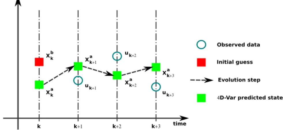
2.1 Principle of data assimilation by means of the 4D-Var approach. . . 19

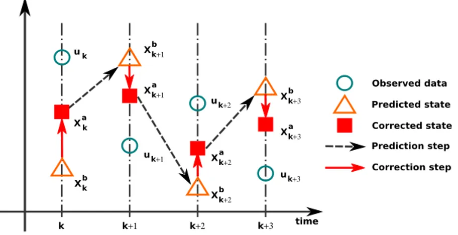
2.2 Principle of data assimilation by means of the Kalman filter approach. . . 21

2.3 Sequential linear Kalman filter equations. . . 21

2.4 Sequential Extended Kalman filter equations. . . 24

2.5 Illustrative comparison between the Unscented and linearization methods for nonlinear stochastic transformations. . . 25

2.6 Tube to support plates gap identification problem in steam generators. . . 26

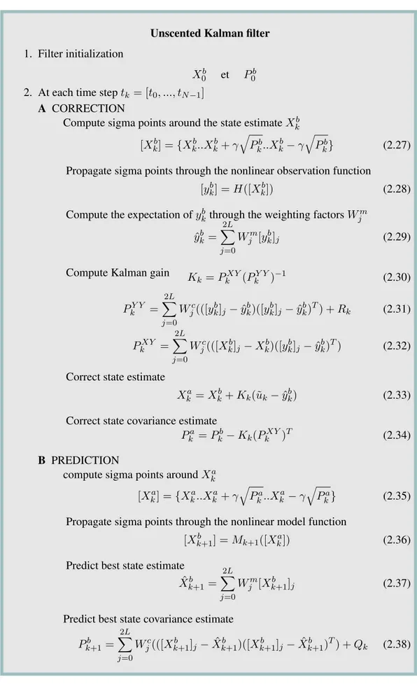
2.7 Sequential Unscented Kalman filter equations for nonlinear system estimation. . . 27

2.8 Evolution ofFfluid(t) and Fcontact(t, q1) in a simulation used to obtain synthetic measurements. . . 28

2.9 Contact gap parameter identification using the Unscented Kalman filter. . . 30

2.10 Unobserved N1 displacement identification using the Unscented Kalman filter. . . 31

3.1 General scheme for the combined use of Error in Constitutive Relation (ECR) and Kalman Filtering (KF). . . 36

3.2 Overview of the preliminary ECR analysis to improve a priori model error knowledge. . . . 38

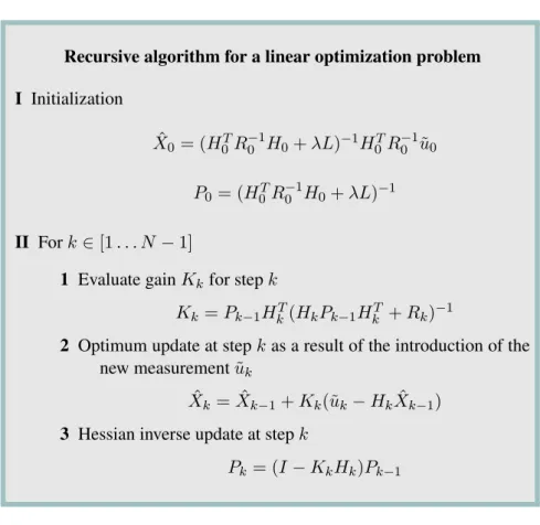
3.3 Recursive algorithm solving a least square optimization problem for linear systems. . . 40

3.4 Linear Kalman Filter algorithm for parameter identication. . . 41

3.5 Extended Kalman Filter algorithm for parameter identification. . . 42

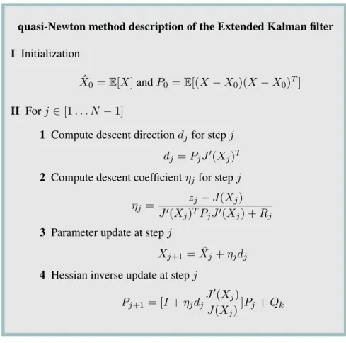
3.6 Description of the EKF for parameter identification as a quasi-Newton method. . . 43

3.7 Description of the Unscented Kalman filter with ECR cost functions in observation space for min-imization purpose. . . 46

3.8 FE model used to generate synthetic measurement data. . . 47

3.9 Admissible fields_{{u − v} and {u − w} minimizing the ECR cost function. . . .} 48

3.10 Distribution of IndKEand IndMEerror indicators over the reference FE model. . . 49

3.11 Identification of damage parameters with the ECR-UKF algorithm. . . 50

3.12 Identification paths over ECR cost function using UKF algorithm for two different initial guesses ofθ0. . . 50

3.13 Identification of model parametresθ defined in (3.23) by means of the ECR and UKF coupled strategy. . . 51

3.14 Comparison ofξ2 T r(θj) residual along the identification process for Extended Kalman filter and Unscented Kalman filter. . . 52

3.15 Comparison of the parameter θ Mean Square Error (MSE) when applying UKF with ECR or Boolean observation operators. . . 52

iv LIST OF FIGURES

3.16 Identification of model parametersθ defined in (3.23) with UKF with the Boolean observation

operatorΠ. . . 53

3.17 General overview for model state and parameter estimation combining ECR and Unscented Kalman filter. . . 54

4.1 Power plant cooling tower FE model used to generate synthetic measurement data. . . 56

4.2 ECR spectrum for reference cooling tower FE model and consequent choice of weighting function η(ω). . . . 58

4.3 Results of the preliminary ECR analysis over the power plant cooling tower FE model. . . 58

4.4 ECR-UKF approach for damage identification of a power plant cooling tower based in a ECR preliminary analysis. . . 59

4.5 Comparison of the eigenfrequencies relative error of the a priori FE model, the identifiedzone1 + zone2 and the separately identified zone1-zone2 models with respect to real eigenfrequencies. . . 60

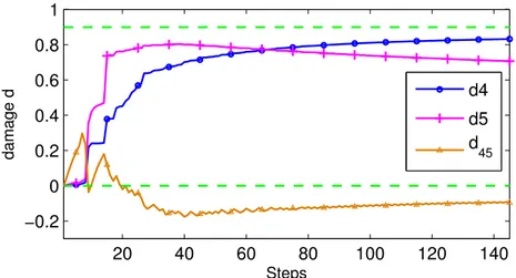
4.6 ECR-UKF approach for time-varying damage identification of a power plant cooling tower. Dam-age region is based on the ECR preliminary analysis of Figure 4.3. . . 61

4.7 Influence of the covariance matrix_Qj in time-varying damage identification using the ECR-UKF approach for a power plant cooling tower. . . 62

4.8 FE model of a concrete beam containing imperfect clamping used to generate synthetic data. . . . 63

4.9 ECR spectrum for perfect double-clamped FE model. . . 64

4.10 Preliminary ECR analysis for a perfect double-clamped concrete beam FE model. Distribution of IndK and IndM estimators over the structure at 80Hz. . . . 64

4.11 Preliminary ECR analysis for a perfect simple-clamped concrete beam FE model. Distribution of IndK and IndM estimators over the structure at 80Hz. . . . 65

4.12 Identified boundary displacements in z direction for the erroneous clamping DOF. . . 66

4.13 Identified impedance in z direction for the erroneous clamping degrees of freedom. . . 67

4.14 Identification of boundary impedance parameters through the ECR-UKF method. . . 68

4.15 Identification path of impedance parameters over the ECR cost function. . . 68

4.16 FE model of a concrete beam containing imperfect clamping and structural damage used to gener-ate synthetic data. . . 69

4.17 ECR spectrum for perfect clamped FE model. . . 69

4.18 Preliminary ECR analysis for a perfect double-clamped concrete beam FE model. Distribution of IndK and IndM estimators over the structure for different frequencies. . . . 70

4.19 ECR analysis for a perfect simple-clamped concrete beam FE model. Distribution of most relevant ECR error indicators. . . 70

4.20 Identified boundary displacements in Z direction for the erroneous clamping DOF in presence of structural damage. . . 71

4.21 Identifiedqˆb/ ˆFbin Z direction for the erroneous clamping DOF in presence of structural damage. 72 4.22 Identification of damage and boundary impedance parameters with the ERC-UKF approach for different parametrization of updating vectorθ. . . . 73

4.23 Identification of damage and boudanry impedance parameters with the ERC-UKF approach for the case of evolving damage and a model parametrization described in (4.19). . . 74

4.24 Block diagram of dual Linear and Unscented Kalman filtering (KF-UKF) for respectively state and parameter estimation. . . 79

4.25 Comparison of identifiedd3damage parameter using dual KF-UKF and joint EKF filtering. . . 79

4.26 Comparison of identifiedq_bjunknown boundary displacement using dual KF-UKF and joint EKF filtering. . . 80

4.27 Identified unknown external effortF_ijwith the dual KF-UKF approach. . . 81

4.28 Illustrative example of a 1D structure deflectionuˆωover the structure length. . . 84

4.29 Illustration of the correlation matrixC shape for a 1D example. . . . 84

LIST OF FIGURES v

4.31 Sequence of state estimation quality during the damage and boundary impedance parameter iden-tification process of the concrete beam example. Comparison ofκ criterion between initial guess,

ECR and BLUE estimators. . . 88

4.32 Sequence of state estimation quality during the damage parameter identification process of a cool-ing tower example. Comparison ofκ criterion between initial guess, ECR and BLUE estimators. . 89

4.33 Cooling tower state estimation error fields at 2.47Hz at first parameter iteration of the ECR-UKF identification process . . . 90

4.34 Cooling tower state estimation error fields at 2.47Hz for FEM with a global Young’s modulus of E= 5E0. . . 91

5.1 Variable transformation T used to introduce algebraic constraints in the framework of the Un-scented Kalman filter for the identification of structural parameters. . . 96

5.2 Identification of structural damage and impedance parameters incorporating parameter constraints with a variable transformation approach for different initial conditions. . . 96

5.3 Modification of the ECR observation operatorξ2 T r(·) with a penalty function depending on the parameter penetration into the inadmissible space. . . 98

5.4 Identification of structural damage and impedance parameters incorporating parameter constraints with a sigma points projection approach for different initial conditions. . . 99

5.5 Modified ECR-UKF algorithm taking into account algebraic state interval constraints. Algorithm steps including a modification of the original UKF are colored in red numbers. . . 100

5.6 Comparison ofξ2 T r(θj) residual along the ERC-UKF identification process for different values of υjin aQj = υj10 −5 I modeling (Type A). . . 102

5.7 Comparison ofξ2 T r(θj) residual along the ERC-UKF identification process for different values of κjin aQj= κjPjθmodeling (Type B). . . 103

5.8 Comparison ofξ2 T r(θj) residual along the ERC-UKF identification process for different values of µjin aQj = µ diag(Pjθ) design (Type D). . . 104

5.9 Comparison ofξ2 T r(θj) residual along the ERC-UKF identification process for different values of αRM in a Robbins-Monro modeling ofQj(Type C). . . 105

5.10 Comparison ofξ2 T r(θj) residual along the ERC-UKF identification process for different designs of error noise covariance matrix_{Q: type A (υ = 0.1), type B (κ = 0.5) and type D (µ = 1.0). . . 105}

5.11 Comparison of the identification results using the ERC-UKF strategy for different modeling of error noise covariance matrix_{Q. . . 106}

5.12 Comparison ofξ2 T r(θj) residual along the ERC-UKF identification process for different designs of error noise covariance matrix_{Q in the case of evolving structural damage: type A (υ = 0.1), type} B (κ = 0.5) and type D (µ = 1.0). . . 106

5.13 Comparison of the identified damage parameterd3along the ERC-UKF identification process for different modeling of error noise covariance matrixQ in the case of evolving structural damage. . 107

6.1 Nuclear auxiliaries building models subjected to seismic loads used in the SMART benchmark. . . 112

6.2 Results of parametric model error localization by means of ECR indicators. Application to differ-ent size and location defects. . . 113

6.3 Results of an ECR analysis use to spatially localize nonlinear structural behavior (damage law). . 113

7.1 Sketching of the reinforced concrete beam test setup. . . 116

7.2 Test setup of the reinforced concrete beam with boundary coupling. . . 117

7.3 Vertical excitation power-spectrum . . . 117

7.4 Concrete beam FE mesh description and sensor locations. . . 118

7.5 Comparison between measured and initial perfect clamped FEM FRFs at sensor S9. . . 119

7.6 Initial ECR spectrum for a perfect double-clamped FEM. . . 119

7.7 Preliminary ECR analysis for a perfect double-clamped concrete beam FE model. Distribution of IndK estimators over the structure at peak error frequencies. . . 120

vi LIST OF FIGURES

7.8 Illustration of initially clamped DOFs condensation into a single DOF containing vertical (z) and rotational (Rx) motion. This model is adopted at each of both clampings. . . 121 7.9 Identified boundary impedances of the concrete beam setup. . . 122 7.10 FRF’s comparison between measured and FEM with identified boundary impedances at sensor S8

location (unobserved). . . 122 7.11 Comparison of ECR spectrum between a perfect clamping FEM and an identified boundary impedance

FEM. . . 123 7.12 ECR analysis for the reinforced concrete beam FE model with boundary impedances. Distribution

ofIndK estimators over the structure at relevant peak error frequencies. . . 123

7.13 Comparison of ECR spectrum between FEMs with Least Square based and ECR-based boundary impedances. . . 126 7.14 Material parameter updating with the ECR-UKF approach. . . 126 7.15 Comparison of ECR spectrum between FEMs with L2-based and ECR-based boundary impedances. 127 7.16 FRF’s comparison between measured and FE models (initial and updated) with ECR based

bound-ary impedances at sensor S8 location (unobserved). . . 128 7.17 Comparison of ECR spectrum for a model with 4 boundary DOFs and the new 16 DOFs boundary

model. . . 129 7.18 Introduction of a quasi-static load producing structural damage (cracks) at the beam’s mid-span. . 129 7.19 Comparison of the ECR spectrum for the reference and the most damaged speciment using

identi-cal boundary impedance functions. . . 130 7.20 Comparison of increment of ECR spectrum∆ξ2

rωfor different levels of structural damage. . . 130

C.1 Illustrative comparison between the Unscented and linearization methods for nonlinear stochastic transformations. . . 146 D.1 Numerical routines work-flow for solving the ECR problem within the Code Aster FE software. . 149 D.2 Implementation of the ECR-UKF algorithm for parameter identification. . . 150

Notations

This section summarizes the conventions and notations used in the sequel. Possible alternate uses of the ensuing definitions are explicitly stated where applicable.

N _{Euclidean space of natural numbers} Rd _{Euclideand-space of real numbers} Cd _{Euclideand-space of complex numbers}

M(K)m,n Space of (m× n) matrices whose entries are in K

Ω Background elastic or viscoelastic solid

E Sub-structure of the elastic or viscoelastic solid

δij Kronecker symbol

In Identity matrix of sizen× n

0n Square zeros matrix of sizen× n

E_{[·] Expectation operator} E Young modulus ν Poisson’s ratio d Structural damage ̺ Mass density σ Stress tensor ε Deformation tensor C Constitutive law t Time variable ω Angular frequency ˜

u Vector of measured displacements ˜

f Vector of measured efforts [M ] Finite Element mass matrix [C] Finite Element damping matrix [K] Finite Element stiffness matrix {F } Finite Element external forces vector {q} Finite Element nodal displacement vector

Π Projection operator from the semi-discretized FE space to the observation space

F

Global Finite Element matrix assembly operator

Xb A priorior background system state vector vii

viii NOTATIONS Xa _{Analyzed system state vector}

M (·) Generic state-transition operator

H(_·) Generic observation operator

Q Covariance matrix of model errors

R Covariance matrix of observation errors

Pb _{Background state error covariance matrix}

Pa _{Analyzed state error covariance matrix}

K Kalman gain matrix

W Unscented sigma weighting factor

γ Unscented sigma point scaling factor

α Spread controlling parameter in sigma point construction for the Unscented transformation

κ Secondary parameter in sigma point construction for the Unscented transformation [Xb_{] Unscented transformation sigma points around background state vectorX}b

[yb_{] Observable transformed sigma points through the observation functionH(·)}

U Space of admissible displacements S Space of admissible stresses

u Kinematically admissible field

v Dynamically admissible field associated to internal efforts

w Dynamically admissible field associated to inertial efforts ˆ

u Optimal kinematically admissible field ˆ

v Optimal dynamically admissible field associated to internal efforts ˆ

w Optimal dynamically admissible field associated to inertial efforts

ξ_ω2(_·) Drucker inequality function at angular frequencyω ξ2

ωr(·) Relative Drucker inequality function at angular frequencyω

[G]R Observation weighting positive-definite matrix of ECR functionals

e2_ω Drucker inequality function at angular frequencyω ξ2

T r(·) Weighted relative Drucker inequality function for a frequency range of interest

η(ω) Weighting function defined over a frequency range of interest Tω Triple of best admissible fields

r Weighting scalar of the ECR functional

ξ2

T r Modifiedξ2T r(·) function including algebraic constraints

E _{Set of potential incorrectly-modeled regions selected for model updating}

θ Vector of model-updating parameters ˆ

θ Optimal vector of model parameters

Q Stationarity error covariance matrix in the state-space description using ECR functionals R Observation error covariance matrix in the state-space description using ECR functionals

ζ Target value of the state-space description using ECR functionals

ϑ Scaling factor of state estimation error covariance matrices

Σ Standard deviations diagonal matrix for the construction ofPb_{in a decomposotion design}

C Matrix of spatial correlations for the construction ofPb_{in a decomposotion design}

Introduction and general overview

EDF group is the first European producer of electric energy with a power capacity of 96 GW installed in France in 2010. Electricity production uses thermal combustion (14%), renewable energies (21%) and nuclear fission (65%). Within the framework of its industrial activity, EDF takes a major place not only in the energy generation field but also in all the main activities related to the electrical industry, namely the transmission, distribution and commercial areas.

One of the priorities of the group is to guarantee the safety of the generation plants, without forgetting the industrial need of maintaining high efficiency. In this context, the EDF research division (R&D) plays a major role in the decision-making of the group, acting as a guarantor for the suitability of the long-term strategies but also taking part in the resolution of in-operation issues during exploitation. As a component of EDF R&D, the Mechanics and Acoustics Analysis department (AMA) provides the expertise in the field of structural mechanics through a wide-scope of research activity (rupture, fluid-structure interaction, vibrations, seismic, rotor-dynamic machines, etc.) from both the computational and experimental viewpoints.

This work arises from AMA department’s need to improve solution methodologies for inverse prob-lems in structural dynamics.

EDF’s industrial need

The AMA department frequently faces dimensioning, monitoring and diagnosis problems, particularly in the field of structural vibrations. In many cases, experimental information is combined with numerical simulations to complete the a priori knowledge of structural behavior in an effort to address industrial issues. Expertise in vibrations is required for a broad range of needs such as health monitoring, structural modification assessment or boundary conditions identification.

Consequently, numerical models must be of good quality in order to accurately predict the behavior of analyzed structures. To this end, experimental data is generally used for model-updating or field reconstruction purposes. Up to now, the AMA department has generally relied on least-square’s type methods to solve identification problems. Moreover, due to the industrial context when studying in-operation structures, linear Finite Element (FE) models are often employed for the sake of reactivity.

In the present work, we investigate alternative solution methods for the above-mentioned problems ix

x INTRODUCTION AND GENERAL OVERVIEW

in the particular industrial context of EDF. More specifically, we aim at studying the dynamic behavior of a generic structure whose available linear FE model_{M has the well-known form:}

[M ]{¨q}(t) + [C]{ ˙q}(t) + [K]{q}(t) = {F }(t) (1)

where[M ], [C] and [K] represent the mass, damping and stiffness matrices respectively,_{{q} is the vector} of nodal displacements and{F } the vector of external loads. Besides, the FE model is supposed not to be inconsistent with a set of available experimental data u for the same structure, and consequently to˜ embed modeling inaccuracies which are a priori unknown.

Hence, the goal of this work is to provide a general method to improve the a priori knowledge of the dynamic behavior of a structure from both an inaccurate FE modelM and a set of available experimental datau. This general goal is formulated in terms of the following three main objectives:˜

1. Identify model inaccuracies and improve the knowledge of the structure’s dynamical behav-ior.

The a priori model_{M is supposed to inaccurately predict the real structure’s dynamics and} there-fore contains model bias. In the present work, we will postulate that such an uncharacterized bias is of a parametrized formM(θ) where θ represents a vector of model parameters (e.g. material parameters, boundary conditions, etc.). In other words, the model inaccuracy is assumed to be attributable to incorrectly-known values of a set of model parameters. Thus, with the help of a set of available experimental datau, we will seek to both identify the nature of the parameter bias (in˜ terms of spatial location and magnitude) and provide a response field estimation.

2. Take into account the case of evolutionary mechanical properties.

In some industrial cases, mechanical properties may evolve during in-operation conditions. In-deed, in some cases EDF has to deal with situations when, for example, investigating whether power plant structures suffer from structural damage during operation (seismic activity, extreme loads, etc.), or evaluate time-varying parameters of rotor-dynamic machines which are usually a function of the rotational speed. In other cases, structures may suffer from structural modifications (boundaries, etc.) as a consequence of maintenance periods. In this work, we will aim at taking into account the possibility of evolutionary structures in two different configurations:

Case A The structure evolves between two or more events well-separated in time and we aim to identify and quantify the total change undergone between these two events. Thus, the evolu-tion law is not necessary sought and parameters will be treated as invariant when modeling each event (e.g. case of changing properties due to maintenance operations).

Case B Structural parameters evolve during the studied event. Consequently, we aim not only to identify parameter overall changes but also to estimate its evolution, which is supposed a

xi

3. Investigate and develop methods applicable to industrial analyses.

Aside from the industrial relevance of the studied problems, the investigations carried out in this work aim at being capitalized for further use in engineering situations. Thus, all the techniques must be applicable to complex structures within moderate computational cost. For this reason, numerical simulations are carried out within the environment of the public FE software Code Aster (www.code-aster.org) developed by EDF R&D.

Considered methods

The choice of the considered methods directly stands from the three main targets defined above. From a general point of view, one can see that we seek to give the best state and parameter estimation in structural dynamics problems from both a (FEM-based) mathematical model and a set of available experimental data. Moreover, since model_{M(θ) is supposed to contain bias error, its a priori predictions are improved} and corrected by taking advantage of experimental (noisy) data.

Consequently, this work aims at solving a category of inverse problems where the existence of both model and observation errors need to be taken into account. Inverse problems have been largely stud-ied within the last decades in a wide range of applications. The reader may find a general overview describing general theory and inversion techniques in [80]. More specifically in structural mechanics, a general description of inversion methods can be found in [16,13] or [91]. Depending on the nature of the inversion problem, specific theories have come to light, for instance the Bayesian approach described in [65] extending the inversion theory to a probabilistic framework.

In this work, Data Assimilation (DA) techniques have been investigated as a way to address inverse problems related to the three above-described main objectives. DA aims at providing optimal state and parameter estimation from the conjunction of uncertain experimental and numerical information. In that sense, model and measurement errors are naturally taken into account, conveniently addressing the first of our targets. Initially introduced in control theory as a method to track model changes in dynamical systems, DA techniques have been widely and successfully used in the past two decades in problems with strong time-varying systems, particularly in the area of geophysics (atmosphere, ocean). DA thus opportunely suits our need of studying evolutionary mechanical properties.

Data Assimilation techniques, however, require good characterization of model and measurement errors (a priori error knowledge) to provide proper system estimations. In the problems we want to address, the a priori knowledge of modeling errors can be quite poor. We therefore enrich it by means of the Error in the Constitutive Relation (ECR). The ECR belong to the category of inverse problems based on energy functionals and represents an alternative to the classical least-square or reciprocity methods in structural mechanics. In particular, the ECR presents interesting features that we propose to exploit such as the ability to spatially localize model errors or the good (empirically observed) convexity properties of cost functions near local minima.

xii INTRODUCTION AND GENERAL OVERVIEW

Overview of the thesis

In light of the above topics and issues, this dissertation is divided into three parts. Part I gives an in-troduction to Error in Constitutive Relation (ECR) and Data Assimilation (DA) techniques where the formulation details and the interesting features of each approach are developed.

In the second, central, part of this dissertation, a general strategy combining DA and ECR methods is proposed. While the first chapter of part II is devoted to building the proposed method, a second chapter puts the strategy at work on problems of industrial relevance, such as structural damage assessment, boundary conditions mis-modeling or field reconstruction. Finally, a third chapter proposes various improvements of this approach, in particular studying the possibility of introducing constraints in the Unscented Kalman filter framework and the influence of the covariance matrices design.

The third and last part of this thesis is devoted to assessing the capabilities and robustness of the combined approach when applied to industrial complex problems. Two different applications are exam-ined. The first one investigates the use of the ECR as a method to localize and characterize structural damage. It is based in the so-called SMART international research benchmark started in 2007 by EDF and CEA (the French Atomic Energy Commission) aimed at assessing the resistance of civil engineering structures to seismic activity. The second application is devoted to an experimental campaign where a reinforced concrete beam is placed in a testing bench that strongly modifies its dynamic behavior. The combined approach is used to identify initially mis-modeled boundary conditions and improve the FE model representativity.

Part I

Introduction to Error in Constitutive

Relation and Data Assimilation methods

Chapter 1

Identification methods and Error in

Constitutive Relation

Contents

1.1 Reference Problem . . . 3 1.2 Energy-based functionals. Introduction to the Error in Constitutive Relation . . . 6 1.3 Conclusions . . . 14

1.1

Reference Problem

In the general framework of nature’s physics, and in particular in solid mechanics, it is often necessary to evaluate or identify physical quantiti es governing a system of interest. In many cases, the sought-after quantities (Young’s modulus, damping coefficients, etc.) may not be directly measurable and one has to exploit other, measurable, quantities (accelerations, deformations, etc.) for the purposes of gaining information. The principle of identification methods consists in establishing a mathematical relation based on physical laws, also known as the model, linking both measurable and non-measurable quantities in a way that the sought-after quantities (in some cases referred to as parameters) can be found from the available measurements. Thus, from a mathematical point of view, the solution of such a problem may encounter problems of existence, uniqueness and continuity of the solutions [13]. Hence, identification methods may be considered in the category of inverse problems where, in contrast with the resolution of a direct problem as illustrated in Figure 1.1, the problem of ill-posedness has to be overcome.

4 CHAPTER 1. IDENTIFICATION METHODS

Figure 1.2: Definition of the studied domain and its boundaries from available data.

From the mechanical point of view, the reference problem we aim to solve consists of studying the evolution of a structure occupying a volumeΩ represented in Figure 1.2 in a time interval t_{∈ [0, T ].}

The structural behavior is given by the solution of the reference problem defined by:

Find the displacements u(z, t) ∈ U(¯u) and stresses σ(z, t) ∈ S( ¯f )∀t ∈ [0, T ], ∀z ∈ Ω verifying the following relations:

- Equilibrium

− ρ¨u(z, t) + div(σ(z, t)) = 0 (1.1)

- Constitutive relation

σ(z, t) =_{C(ε(u(z, t)), θ)} (1.2) whereε is the strain tensor and θ represents a given set of model parameters defining the structural

prop-erties (material, geometry, etc.). Moreover, the space of admissible displacementsU(¯u) and admissible stresses_{S( ¯}f ) are defined by:

(

U(¯u) = {u(z, t) s.r. |u(z, t) = ¯u for z ∈ ∂uΩ and u(z, 0) = u0, ˙u(z, 0) = ˙u0}

S( ¯f ) =_{{σ(z, t) s.r. |σ(z, t) · n = ¯}f for z_{∈ ∂}fΩ}

(1.3)

where “s.r.” denote sufficiently regular functions defined onΩ of bounded strain and kinetic energy for

u(z, t) and square-integrable for σ(z, t), and n is the normal vector to the surface ∂Ωf.

The problem is said to be well-posed in the sense of Hadamard [16] if, and only if, the three following conditions are verified:

1. A solutionu(z, t) exists∀z ∈ Ω, ∀t ∈ [0, T ] for given ¯u and ¯f .

2. The solutionu(z, t) is unique.

3. The solution depends continuously onu and ¯¯ f .

Well-posedness requires in particular∂Ω = ∂uΩS∂fΩ and ∂uΩT∂fΩ = ∅ (with reference to

Figure 1.2). In this description, the direct problem will be generally ill-posed for at least two reasons: 1. The presence of overdetermined datau and ¯¯ f in ∂f uΩ generally leads to the non-existence of the

1.1. REFERENCE PROBLEM 5 2. The lack of data in a certain region of the boundary∂0Ω can lead to non-uniqueness. This will

be particularly the case when ∂f uΩ = ∅. In this case, prescribing either force or displacement

boundary data on∂0Ω restores well-posedness.

In our case, we will seek to find the set of model parametersθ and the solution field u satisfying

the above model equations (1.1) and (1.2) that better represents the available data. Since the available datau and ¯¯ f might be noisy and overdetermined, and the model equations inaccurate with respect to real

physics (domain discretization, material,etc.), the solution of this inverse problem might be in many cases ill-posed in the sense of Hadamard as it may not respect one or more of the above-listed conditions. In the field of solid mechanics, many authors have investigated the identification of model properties from observed data. To give an example, it has been shown in [20,14] that, in the elastic case, the problem of finding a field of distributed properties E(z) in the whole space Ω is an ill-posed problem in the sense of Hadamard and the introduction of an a priori knowledge that approximates the solution is mandatory.

Several methods exist for solving problems of model properties identification, depending on the nature of the problem (statics, dynamics, available data, etc.). The identification problem generally ends up being formulated as an optimization problem, namely seeking the minimum of a cost function that quantifies in a certain metrics the difference between a model prediction and the available data.

Among the different existing approaches for building suitable cost function, the following families can be distinguished:

• The least-squares approaches [81] where the difference between data and the direct model solution projected onto the observation space is measured with aL2 _norm.

• An approach based on auxiliary fields. In linear mechanics, these approaches exploit the Maxwell-Betti reciprocity theorem and generally cost functions are built upon the overdetermined data over the boundary domain. An interesting example using this approach can be found in [3] for crack detection inside an elastic body.

• An approach consisting on energy-based functionals, and particularly those based in the Error in Constitutive Relation (ECR) for which a detailed description is given later.

On the other hand, the ill-posedness of the identification problem will generally lead to sensitivity or instability of the solutions with respect to noisy data. To overcome this issue, we will distinguish between two classical approaches:

• The widely used Tikhonov regularization techniques ([84], [13]) where an additional term is intro-duced in the aforementioned cost functions. This term represents an a priori knowledge about the sought-after solution and has the property to stabilize the results with respect to noise in data. • The probabilistic approaches [80,24,6] where data and model uncertainties are quantified using

a stochastic framework, and a probability density function for the unknown parameters is usually sought.

In the next section, a more in-depth description of ECR-based identification methods is provided. For more information on inverse problems, the reader can find a general overview in [13,81,80] and in particular for structural mechanics in [14,16].

6 CHAPTER 1. IDENTIFICATION METHODS

1.2

Energy-based functionals. Introduction to the Error in Constitutive

Relation

In the case of the least-squares or the auxiliary fields approaches, the quality of a model is measured by either the distance between the measured data to the solution of the direct problem or the reciprocity gap. On the contrary, the energy-based functionals propose to measure the model error by evaluating the difference between kinematically and statically admissible fields using an energy norm. Finding the best admissible fields itself leads to the resolution of a secondary problem, leading to a two-step inverse solution procedure for the general identification process.

This technique has first been introduced by P. Ladev`eze in 1975 as a method to evaluate the quality of the solution of a FE model [55], where the concept of Error in constitutive Relation (ECR) first appeared. Since then, several versions and many applications have been proposed, see for example [57,60,70] for model quality assessment or [19,37,42,2,67,26] for model updating and identification problems.

The background idea of Error in Constitutive Relation can be introduced from two different points of view:

• A first approach valid for Generalized Standard Materials (GSM) [43]. For such materials, the constitutive equations are described from the expressions of the energy potential and the dissi-pation potential. The difference between two admissible states associated with both force and displacement boundary conditions are characterized by the residual:

e(ε, σ) = φ(σ) + φ∗(ε)_{− σ : ε} (1.4) where φ∗ is the potential defined by the Legendre-Fenchel transformation of φ. In the case of

elasticity, those potentials are defined by:

φ(σ) = 1

2σ

T_K−1_{σ, φ}∗_{(ε) =}1

2ε

T_{Kε (1.5)}

where K is the Hooke tensor. This error is positive-definite and vanishes when the admissible

states are compatible with the constitutive relation. Thus, it can be used as a measure to build ECR functionals.

• The second point of view comes from the principle of stability in the sense of Drucker which, for a given structure, stipulates that for any couple of evolution states (considering the same initial state) the following inequality stands:

Z T

0

Z

Ω(σ2− σ1) : (ε2− ε1)dzdt≥ 0 ∀t ∈ [0, T ], ∀z ∈ Ω (1.6)

It can be shown that the Drucker error vanishes for the case where the two couples (σ1, ǫ1) and

(σ2, ǫ2) are compatible with both the history of boundary conditions and the constitutive relation,

1.2. ERROR IN CONSTITUTIVE RELATION 7 of a given structure is unique for all evolution coming from the same boundary condition history. This uniqueness property is verified in most of the constitutive relations such as elasticity, plastic-ity, viscoelasticplastic-ity, etc. except from some singular cases (damage laws). Indeed, the integration of the virtual work equations for a given structure gives:

Z T 0 Z Ω (σ2− σ1) : (ε2− ε1)dzdt + Z T 0 Z Ω 1 2ρ( ˙u1− ˙u2) 2_{dzdt = 0 (1.7)}

and considering the Drucker inequality (1.6) one can easily obtain:

Z

Ω

1

2ρ( ˙u1− ˙u2)

2_{dzdt≤ 0 ∀t ∈ [0, T ], ∀z ∈ Ω (1.8)}

Hence, it is clear that for a given structure ˙u1 and ˙u2 are necessarily the same for allt ∈ [0, T ]

as the two evolutions have the same initial condition. Thus, deriving this expression, the history of deformations must be identical and so has to be the history of constrains from the constitutive relation law. This hypothesis has therefore been exploited to define a residual indicator based in the Drucker inequality as a measure of the compatibility of the constitutive relation of a structure with respect to the boundary conditions.

Since the introduction of such a concept, several studies have successfully applied this principle to different applications such as model verification [58] and model updating problems [56, 59], under linear or nonlinear conditions [10,19], either in the frequency domain [27] or the time domain [36,37]. Consequently, the constitutive relation appears to be an appropriate indicator of the quality of a model with respect to measured data history and some particularly good properties deserve to be highlighted:

• Excellent ability to locate erroneously modeled regions in space. Indeed, in [10] it is demonstrated that regions where the ECR density is high correspond to those which contain the most erroneous constitutive relations.

• Strong robustness in presence of noisy data [37]. • Good convexity properties of cost functions [42].

In the following, classical formulations of the ECR are reviewed for the static and the dynamic cases. Moreover, a frequency domain formulation is presented with a special interest for the case of a FE framework.

Classic formulation. The static case.

In the field of static elasticity, the ECR can be formulated in one of its most classical forms. Consider the case where∂0Ω =∅ and ∂ufΩ6= ∅. Thus, the elasticity tensor C that better represents the available

8 CHAPTER 1. IDENTIFICATION METHODS

Find the kinematic admissible fielduKA ∈ U(¯u), the static admissible field σSA ∈ S( ¯f ),

and the constitutive relation_{C that minimize:}

J(uKA, σSA,C) =

Z

Ω(σSA− C : ε(uKA)) :C

−1 _{: (σ}

SA− C : ε(uKA))dΩ (1.9)

where the admissible spaces are defined by:

(

U(¯u) = {u(z) s.r. |u(z) = ¯u for z ∈ ∂uΩ}

S( ¯f ) =_{{σ(z) s.r. |σ(z) · n = ¯}f for z_{∈ ∂}fΩ, div(σ(z)) = 0 for z ∈ Ω}

In this static case, it can be shown that the solution fieldsuKA andσSAare uncoupled. In practice,

this means that both fields can be computed separately as a Neumann and a Dirichlet problem respec-tively.

Modified formulation. The dynamic case.

In the case of elastodynamics, nevertheless, it has been proved in [36,2] that the resolution of an ECR introduces an additional issue since the kinematic and dynamically admissible fields are coupled not only by the constitutive relation (1.2) but also by the equilibrium equation (1.1). In addition, a regularization technique is introduced to deal with the presence of noisy measurements. In this context, a modified approach has been proposed by Feissel and Allix in [36]. In their investigations, they considered the case with∂0Ω =∅ and ∂fΩ = ∂uΩ = ∂f uΩ. Their formulation of the ECR problem is summarized below:

Find the kinematic admissible fielduKA ∈ U(ub), the dynamic admissible field σDA ∈ S(fb, u), and

the constitutive relationC that minimize:

J(uKA, σDA,C) = Z T 0 Z Ω(σDA− C : ε(uKA)) :C −1 _{: (σ} DA− C : ε(uKA))dΩdt + Z T 0 Z ∂uΩdu(ub, ¯u)dS + Z ∂fΩ df(fb, ¯f )dS ! dt (1.10)

where the admissible spaces are defined by:

(

U(ub) ={u(z, t) s.r. |u(z, t) = ub for z∈ ∂uΩ, u(z, 0) = u0, ˙u(z, 0) = ˙u0}

S(fb, u) ={σ(z, t) s.r. |σ(z, t) · n = fbforz∈ ∂fΩ, −ρ¨u(z, t) + div(σ(z, t)) = 0 for z ∈ Ω}

where the termsduanddf represent a discrepancy measure to be defined (usually based on theL2norm,

e.g.du(v, w) =kv − wk2)).

In all the cases, the ECR approach relies upon distinguishing between two sets of relations: reliable and unreliable. The latter will therefore be relaxed by simply introducing them in the ECR functional and finding a solution that best fulfills them. In the case of elastodynamics defined in (1.10) the following sets of relations can be introduced:

1.2. ERROR IN CONSTITUTIVE RELATION 9 • Reliable relations:      −ρ¨u + div(σ) = 0 u(z, 0) = u0 ˙u(z, 0) = ˙u0 (1.11)

• Unreliable relations and quantities:

     σ = Cε ¯ u ¯ f (1.12)

An interesting work by Feissel, Allix and Nguyen in [37,67] has recently shown that in the identifi-cation process by means of ECR functionals, the obtainment of admissible fieldsuKAandσDA and the

correction of the constitutive relation_{C are two well-separated steps and therefore one can use different} functionals to solve each problem. In particular in one of the examples the identification problem is defined as follows:

Given a constitutive relationC, find the fields σDA∈ S(fb, u), uKA∈ U(ub) minimizing

J(uKA, σDA,C) = Z T 0 Z Ω (σDA− C : ε(uKA)) :C−1 : (σDA− C : ε(uKA))dΩdt + Z T 0 Z ∂uΩdu(ub, ¯u)dS + Z ∂fΩ df(fb, ¯f )dS ! dt (1.13) where _S(fb, u) and U(ub) are defined in (1.10) and the functional used to measure the

discrepancy on the constitutive relation is

G(uKA, σDA,C) = Z T 0 Z Ω (σDA− C : ε(uKA)) :C−1 : (σDA− C : ε(uKA))dΩdt (1.14)

This approach has been tested with satisfying results in a 1-D case where the Young’s modulus is sought and the measurement noise reached 60%. Experiments were realized for both homogeneous and heterogeneous moduli. In all the cases, the ECR approach presented excellent properties of robustness against noisy data as well as good convexity properties of cost functions. However, the research per-formed in [36] and [67] clearly pinpointed one of the major limitations of this method: its computational cost when solving the minimization problem. As a matter of fact, the resolution of the ECR problem in elastodynamics leads to a large system of space-time equations where the admissible fields are coupled to the solution of a time-backwards adjoint problem. Hence the application of such a formulation for an industrial size problem is still an area of open research. In the following we will use the frequency domain formulation which is presented below.

Frequency-domain formulation. Application to a FE formulation.

In the scope of the present work and with the aim to avoid prohibitive computational costs that would prevent the use of the ECR in industrial cases, a frequency-domain formulation will be adopted from now

10 CHAPTER 1. IDENTIFICATION METHODS

on. This derivation of the ECR was studied by [19] in a FE framework and further adopted by [26,27] to a high DOF case. Thus, this version of the ECR is the most suitable when dealing with linear FE models of industrial size.

To fix the ideas, consider the above equations (1.1) and (1.2) and assume that the sought-after solu-tions are of the form:

ℜ(uω(z)eiωt), ℜ(σω(z)eiωt) (1.15)

where_{ℜ(·) represents the real part of a complex number and ω is the angular frequency. Then, equation} (1.1) can be rewritten as:

− ρω2uω(z) + div(σω(z)) = 0 (1.16)

When it comes to the constitutive relation, the following expressions are considered:

(

σω(z) = (K + iωC)ǫ(uω(z))

Γω(z) =−ρω2uω(z)

(1.17)

whereΓω represents the inertial forces, andK and C are respectively the Hooke and damping tensors.

From the above equations (1.17), the following spaces are defined:

     U(¯u) = {uω(z) s.r.|uω(z) = ¯u for z∈ ∂uΩ} S( ¯f ) =_{σω(z) s.r. |σω(z) = (K + iωC)ǫ(vω(z)), σ(z)· n = ¯f for z∈ ∂fΩ} D(σ) = {Γω(z) s.r. |Γω(z) =−ρω2wω(z), Γω(z) + div(σω(z)) = 0 for z∈ Ω} (1.18)

whereuω(z), vω(z) and wω(z) are displacement fields and in the sequel will be denoted u, v and

w respectively for the sake of clarity. Thus, the Drucker inequality (1.6) can be rewritten, for a given

angular frequencyω, by considering a triple of displacement fields only, as: ξ2_ω(u, v, w) = Z Ω{ γ 2Trace[(K + T ω 2_{C)(ǫ(v)− ǫ(u))}∗_(ǫ(v) − ǫ(u))] +1− γ 2 ρω 2_{(u− w)}∗_{(u− w)}dΩ} (1.19)

where γ _{∈ [0, 1] is a weighting scalar indicating the relative quality of the constitutive relations}

(1.17) and the superscript “∗” represents the complex conjugate. Hence, from the above definition (1.18) of admissible spaces we will refer tou as a kinematically admissible field, v as a dynamically

admis-sible field related to theK and C tensors and w as a dynamically admissible field related to inertial forces.

Since the expression of the Drucker error has been defined for the frequency domain, the following expressions can be developed in order to be applied for the study of real structures.

A relative structural error can be defined as:

ξωr2 =

ξ2ω

D2

ω

(1.20) whereD2ωrepresents the reference structural energy defined by:

D2_ω= Z Ω (γ 2Trace[(K + T ω 2_C)ǫ(u)∗_{ǫ(u)] +}1− γ 2 ρω 2_u∗_{u)dΩ (1.21)}

1.2. ERROR IN CONSTITUTIVE RELATION 11 Besides, if we are interested in studying the influence of different regions ofΩ to the global error, we might consider a subdivision of sub-domainsE _{∈ E of Ω in a way that Ω =} nSE

i=1

Ei. Thus, the global

error can be interpreted as the contribution of all the local errors and we obtain:

ξ_ωr2 = X

E∈Ω

ξ2_ωEr (1.22)

Moreover, when studying the behavior of a structure in the frequency domain, it is natural to be interested in its behavior in a bandwidth of interest[ωmin, ωmax] of angular frequencies. Thus, we can

define the bandwidth relative error as:

ξT r2 =

Z ωmax

ωmin

η(ω)ξωr2 dω (1.23)

whereη(ω) is a weighting function defined over [ωmin, ωmax] satisfying the following condition:

Z ωmax

ωmin

η(ω)dω = 1 η(ω)≥ 0 (1.24)

In most of the industrial and application cases, and in the particular scope of interest of this work, the study of structural dynamic behavior is performed by means of Finite Element models. In order to adopt the above error expressions in a FE framework, the discretization of equation (1.16) leads to the following matrix equation:

[−ω2[M ] + jω[C] + [K]]{q} = {F } (1.25)

where[M ], [C] and [K] are the so-called mass, damping and stiffness matrices respectively. Moreover, {F } and {q} are the vectors of nodal forces and displacements. Within this framework, the following considerations will be made with regard to the inverse problem we aim to solve:

• ∂0Ω =∅

• The prescribed loading ¯f over ∂fΩ is considered as a reliable information (e.g. external loadings,

free surfaces, etc.) and directly embedded in{F }.

• A set of unreliable displacement data ˜u (e.g. sensor measurement on a free surface) is available over∂f uΩ.

• Displacement data ¯u are restricted to the boundary ∂u\fΩ = ∂uΩ− ∂f uΩ and considered as a

reliable information (e.g. clampings). This reliable kinematic information is generally enforced in the construction of model matrices by either introducing Lagrange multipliers or by considering matrices with active DOFs only, which is the solution adopted in the sequel.

Hence, the above FE matrix equation (1.25) and the Drucker inequality (1.19) leads to the following expression of the modified Error in Constitutive Relation in a FE framework:

12 CHAPTER 1. IDENTIFICATION METHODS

Find the kinematic admissible field u _{∈ U(Π, ¯u), and the dynamic admissible fields (v, w) ∈}

D({F }, ¯u) minimizing: e2_ω(_{{u}, {v}, {w}) =}γ 2{u − v} ∗_{[K + T ω}2_{C]{u − v} +}1− γ 2 {u − w} ∗_ω2_{[M ]{u − w}} + r 1− r{Πu − ˜u} ∗_[G R]{Πu − ˜u} (1.26) where the admissible spaces are defined by:

      

U(Π, ¯u) = { {u} s.r. |PN

i=1uiϕi(z) = ¯u for z ∈ ∂u\fΩ, u(z) = Π{u} for z ∈ ∂f uΩ}

D({F }, ¯u) = { {w}, {v} s.r. |XN

i=1viϕi(z) =

XN

i=1wiϕi(z) = ¯u for z∈ ∂u\fΩ,

[K + iωC]_{{v} − ω}2[M ]_{{w} = {F } }}

where (ϕ1, . . . , ϕN) are the basis functions, r is a weighting scalar, Π a projection operator from

the space of structural nodal displacements to the observation space and[GR] represents a symmetric

positive-definite matrix. Notice that, in this formulation, unreliable displacementsu are introduced as an˜ additional term in the ECR functional (1.26). As described for the dynamic formulation in time domain, this consists of the modified formulation and corresponds to the regularization term stabilizing the solu-tions in case of noisy data (e.g. experimental measurements). Moreover, although the choice of matrix [GR] is not a priori defined it is usually chosen to be dimensionally consistent with the induced energy

norm as proposed in [26,27]. In our case the following choice is made: [GR] = γ 2[[KR] + T ω 2_[C R]] + 1_{− γ} 2 ω 2_[M R] (1.27)

where the index “R” represents the Guyan reduction on the observation space.

Hence, in order to evaluate the discrepancy of a FE model with respect to a set of measurements, a two step method is adopted:

1. Given a set of model parametersθ that parametrize [M ] = [M (θ)], [C] = [C(θ)], [K] = [K(θ)],

obtain the triple of admissible fields Tω = (ˆu, ˆv, ˆw) that minimizes (1.26). This minimization

problem leads to the resolution of linear equations as developed in Appendix B. 2. Evaluate the model error by computinge2

ω(Tω, θ), or its relative forme

2

ω(Tω,θ)

D_ω(ˆ2 _u,θ)

In the present work, we aim not only at studying model errors in a bandwidth of frequencies, but also at monitoring their spatial distribution overΩ. For these reasons, from now on, the following expression is adopted to evaluate the total model error:

ξT r2 = Z ωmax ωmin η(ω)   X E∈Ω e2_Eω(Tω, θ) D2 ω(ˆu, θ)  dω (1.28)

Thus, since the triple of admissible fields solution of (1.26) depends onθ (Tω =Tω(θ)), the problem

of finding the best set of model parametersθ that better represents the noisy data ¯u can be written as:

ˆ

θ = arg min

θ∈Θξ 2

1.2. ERROR IN CONSTITUTIVE RELATION 13 whereΘ is the space of admissible parameters.

The well-behaved nature of functional (1.28) with respect toθ is one of the main features that we aim

to take advantage of in this work. A visual example is presented in Figure 1.3, where aξ_{T r}2 functional is evaluated in a 4-DOF dynamic system for different values of stiffness (k) and mass (m) as described in

Figure 1.3(a), where all displacements are supposed to be observed and the external load is supposed to contain a single frequency. This surface is compared to the one obtained with a least square functional of the formk˜u − Πqdirectk2, whereqdirect represents the solution of the associated direct problem. As it

can be seen in Figure 1.3(b) and Figure 1.3(c), the ECR functional exhibits a clear minimum while the least square surface presents several local minima and peaks.

(a) 4-DOF system definition

1 2 3 1 2 3 100 m /m0 k / k0 (b) ERC functional (ξ2 T r) 1 2 3 1 2 3 m /m0 k / k0

(c) Least squares functionalk˜u− Πqdirectk

Figure 1.3: Comparison between ECR and least squares functionals convexity for a 4-DOF dynamic system varying stiffness (k) and mass (m) parameters.

To conclude with the frequency-domain FE formulation of the ECR, it is important to point out some of its main features that make them particularly interesting for our usage:

• Model data is introduced in this ECR version on the basis of [M], [C] and [K] matrices. Those objects are classically used in FE software, which facilitates the manipulation of ECR concepts. • The adopted ECR formulation is based on displacement fields only. Again, this feature facilitates

14 CHAPTER 1. IDENTIFICATION METHODS

its integration in FE software. The computation ofe2

EωandD2ωis a straightforward calculation of

elementary and/or global energies.

• Large-DOF models can be studied either by using convenient sparse matrix operators or by imple-menting model reduction techniques as proposed in [27].

• Obtaining the triple of admissible fields Tωdoes not require the computation of the adjoint solution

(as required in the time-domain formulation) which in some cases can be a difficult task to perform within the classical FE software functions.

1.3

Conclusions

In this chapter, the general concepts of the Error in Constitutive Relation have been introduced as a suitable basis for identification problems in structural mechanics. The ECR approach is a measure of the discrepancy of admissible fields which can be derived from either the Drucker error or the Legendre-Fenchel error. Here, classical and modified formalisms are presented and, in particular, the adequacy of the FE frequency-domain formulation to industrial contexts is highlighted.

As a matter of fact, ECR-based approaches present specific features that make them particularly attractive when dealing with an identification problem in structural mechanics: good convexity of cost functionals, ability to localize model errors in space, and robustness in the presence of of noisy data. For these reasons, they are adopted in this work as a tool to both enhance the a priori model error knowledge and alleviate the stability problems when performing parameter identification with Kalman filtering (KF), which are presented in the next chapter. Combining Kalman filtering and ECR make up the core of this work and is further developed and studied in part II.

Chapter 2

Data Assimilation

2.1 Introduction . . . 15 2.2 Concepts and classic notation in data assimilation . . . 16 2.3 Sequential and variational formalisms: Kalman filter and 4D-Var . . . 17 2.3.1 Variational formalism: 4D-Var . . . 18 2.3.2 Sequential formalism: The Kalman filter. . . 20 2.4 Example of nonlinear identification by means of the Unscented KF . . . 26 2.5 Conclusions . . . 31

2.1

Introduction

The main purpose of data assimilation (DA) techniques consists of providing a system state estimation from all the available information obtained from both numerical simulation and physical observations of all kinds. Thus, the final aim of all DA techniques is to provide optimal past, present and, most importantly, future state estimations. To do so , many different techniques exist to enrich the system’s theoretical knowledge (also referred to as the a priori knowledge) with the help of available observations. The origins of data assimilation go back to the 1940 decade when Norbert Wiener showed a growing interest to build optimal predictors for stationary time series [89], proposing a first application in the ballistics domain during the Second World War. The Wiener predictors were somehow reviewed during the 1960’s by Rudolph E. K´alm´an to extend the formalism to non-stationary time series, giving birth to the celebrated Kalman Filter (KF) [53].

Since its origins, data assimilation techniques have seen a vast and still growing number of applica-tions, providing a theoretical framework for addressing problems of very diverse nature, such as avionics and spaceship control, medical imaging, neutron transport, optimal interpolation, system identification, etc. Data assimilation can therefore be considered as an approach for solving inverse problems.

Nowadays, DA is widely employed in the domain of external geophysics (weather forecast, oceanog-raphy, etc.) for the purpose of reconstructing the initial state of chaotic systems (Lorenz, atmosphere,