en fr

HAL Id: tel-02007512

https://tel.archives-ouvertes.fr/tel-02007512

HAL is a multi-disciplinary open access

archive for the deposit and dissemination of sci-entific research documents, whether they are pub-lished or not. The documents may come from teaching and research institutions in France or

L’archive ouverte pluridisciplinaire HAL, est destinée au dépôt et à la diffusion de documents scientifiques de niveau recherche, publiés ou non, émanant des établissements d’enseignement et de recherche français ou étrangers, des laboratoires

Self-organizing map quantization error approach for

detecting temporal variations in image sets

John Mwangi Wandeto

To cite this version:

John Mwangi Wandeto. Self-organizing map quantization error approach for detecting temporal vari-ations in image sets. Artificial Intelligence [cs.AI]. Université de Strasbourg, 2018. English. �NNT : 2018STRAD025�. �tel-02007512�

UNIVERSIT´

E DE

STRASBOURG

´

ECOLE DOCTORALE MS2I

ICUBE – CNRS UMR 7357- LABORATOIRE DES SCIENCES DE L’INGENIEUR, INFORMATIQUE ET

IMAGERIE

TH`

ESE

pr´esent´ee

par:

John

Mwangi WANDETO

souten

ue le 14 septembre 2018

pour obtenir le grade de: Docteur de l’Universit´

e de Strasbourg

Discipline/ Sp´ecialit´e: Informatique

Self-Organizing Map Quantization Error Approach for Detecting Temporal Variations in Image Sets

TH`ESE dirig´ee en cotutelle par:

MME Birgitta DRESP Directeur de Recherche, CNRS Strasbourg, FRANCE (Supervisor) M Henry Okola NYONGESA Professor of Computer Science and Systems Engineering,

DeKUT, Nyeri, KENYA (Co-supervisor) RAPPORTEUR-E-S:

M Paul ROSIN Professor of Computer Vision, Cardiff University, UK MME Rachele ALLENA PhD, HDR, MCF ENSAM, Paris, FRANCE AUTRES MEMBRES DU JURY:

M Daniel GEORGE (examinateur) PhD, HDR, MCF Strasbourg University, FRANCE M Jos´e RAGOT (examinateur) Professor Emeritus of Automatics, Nancy University,

Abstract

A new approach for image processing, dubbed SOM-QE, that exploits the quan-tization error (QE) from self-organizing maps (SOM) is proposed in this thesis. SOM produce low-dimensional discrete representations of high-dimensional in-put data. QE is determined from the results of the unsupervised learning process of SOM and the input data. SOM-QE from a time-series of images can be used as an indicator of changes in the time series. To set-up SOM, a map size, the neigh-bourhood distance, the learning rate and the number of iterations in the learning process are determined. The combination of these parameters that gives the low-est value of QE, is taken to be the optimal parameter set and it is used to transform the dataset. This has been the use of QE. The novelty in SOM-QE technique is fourfold: first, in the usage. SOM-QE employs a SOM to determine QE for differ-ent images - typically, in a time series dataset - unlike the traditional usage where different SOMs are applied on one dataset. Secondly, the SOM-QE value is intro-duced as a measure of uniformity within the image. Thirdly, the SOM-QE value becomes a special, unique label for the image within the dataset and fourthly, this

label is used to track changes that occur in subsequent images of the same scene. Thus, SOM-QE provides a measure of variations within the image at an instance in time, and when compared with the values from subsequent images of the same scene, it reveals a transient visualization of changes in the scene of study. In this research the approach was applied to artificial, medical and geographic imagery to demonstrate its performance. Changes that occur in geographic scenes of interest, such as new buildings being put up in a city or lesions receding in medical im-ages are of interest to scientists and engineers. The SOM-QE technique provides a new way for automatic detection of growth in urban spaces or the progressions of diseases, giving timely information for appropriate planning or treatment. In this work, it is demonstrated that SOM-QE can capture very small changes in images. Results also confirm it to be fast and less computationally expensive in discriminating between changed and unchanged contents in large image datasets.

Pearson’s correlation confirmed that there was statistically significant correlations between SOM-QE values and the actual ground truth data. On evaluation, this technique performed better compared to other existing approaches. This work is important as it introduces a new way of looking at fast, automatic change detection even when dealing with small local changes within images. It also introduces a new method of determining QE, and the data it generates can be used to predict changes in a time series dataset.

Keywords: change detection, self-organizing map, quantization error, time series images, change prediction, difficulty to detect changes.

Dedication

To my Dad, Wandeto and my Mum, Wanja for being the most practical problem-solving coaches.

To my family: Mercy, Elizabeth, Ann, Maria and Martha; as you are the world’s greatest team.

Acknowledgements

I would like to acknowledgement Birgitta DRESP and Henry NYONGESA, the supervisors of the development of this thesis. It was largely due to their univo-cal guidance, criticism and encouragement that constant progress was made in the research that culminates in this thesis. In particular, it was encouraging when they promptly replied to my queries, providing clear and straightforward com-ments that ensured smooth planning, implementation, analysis and reporting of the experiments. Special thanks to the French government, who through their embassy in Nairobi, Kenya awarded me the scholarship to study and do this re-search work in France. I also recognize efforts by the two universities involved in this research: Dedan Kimathi University of Technology, Nyeri Kenya and the University of Strasbourg, France. They provided good working environment that enabled timely completion of the studies. I will also like to pass special thanks to two radiologists: Dr. Philippe Choquet (PhD) from Hˆopital de Hautepierre, and ICube UMR 7357 CNRS-UdS, Strasbourg France, who provided valuable insight and expertise for this research, and Dr. Christian Goetz (PhD) also of Hˆopital de

Hautepierre as at December 2015, for playing a crucial role in shaping the idea behind the thesis. Both provided information on how radiologist manage, acquire and utilize information gleaned from images. It was through watching them ma-nipulate medical images, and listening to them talk about gathering information from the images that I gained the confidence and the conviction to work on this thesis. I also thank them for suggesting and directing me to possible and relevant medical image datasets. Last but not least, I thank Yves REMOND, Professor of Mechanics, Strasbourg University, for regularly providing advice on the pro-cess and as the head of the doctoral school, provided guidance on administrative matters pertaining to PhD studies at Strasbourg.

Contents

List of Figures xi

List of Tables xv

1 Introduction 1

1.1 Application of Artificial Intelligence on Images . . . 2

1.2 Review of change detection work . . . 7

1.3 Motivation for this work . . . 15

1.4 Objectives of the study . . . 16

1.5 Statement of the problem . . . 17

1.6 Scope . . . 18

1.8 Limitations . . . 19

1.9 Thesis organization . . . 20

2 Self-Organizing Map and the Quantization Error (SOM-QE) 21 2.1 Brain maps and vector quantization . . . 22

2.2 SOM . . . 25

2.3 SOM learning: winner-takes-all . . . 30

2.4 Network architecture . . . 32

2.5 The trained SOM: final synaptic weights . . . 38

2.6 The quantization error (QE) . . . 41

2.7 The SOM-QE concept . . . 44

2.8 Hypothesis: SOM-QE value reflects critical variations in image content and it predicts future image status. . . 54

3 Experimental Methodology 56 3.1 Change detection problems detectable by SOM-QE . . . 58

3.1.1 Materials and methods . . . 59

3.2 How sensitive is SOM-QE? Comparing SOM-QE to human

de-tection . . . 75

3.2.1 Subjects . . . 76

3.2.2 Materials and methods . . . 76

3.2.3 Results . . . 79

3.2.4 Discussion . . . 89

3.3 Change detection in time series of medical images . . . 90

3.3.1 Materials and methods . . . 94

3.3.2 Results . . . 98

3.3.3 Discussion . . . 102

3.4 Change detection in time series of satellite images . . . 105

3.4.1 Determining urban growth variability through Atlas maps 106 3.4.2 Regions in Las Vegas . . . 107

3.5 Using SOM-QE to tell future occurrences . . . 132

3.5.1 Method . . . 135

3.5.2 Results . . . 136

3.6.1 Carbon dioxide gas measurements . . . 138

3.6.2 Challenging change-detection image dataset . . . 145

3.7 The SOM-QE algorithm: New method to determine QE in time series images . . . 146

3.7.1 Introduction . . . 146

3.7.2 Method . . . 149

3.7.3 Results . . . 150

4 Discussion of results 154

5 Conclusions and Contribution 158

Bibliography 162

Appendix A List of publications the thesis has produced 180

Appendix B Sample code: The Python code used in section 2.7 183

Appendix C Real medical images: set 1 195

Appendix E Real medical images with added 1 ‘lesion’ 201

Appendix F Real medical images with global ‘lesions’ 204

Appendix G Satellite images: Las Vegas City Center ROI 207

Appendix H Satellite images: Lake Mead ROI 210

Appendix I Satellite images: Residential North of Las Vegas ROI 213

I.1 R´esum´e . . . 216

List of Figures

2.1 SOM learning . . . 26

2.2 Reducing sensitivity from point of touch . . . 32

2.3 Trained SOM . . . 40

2.4 Histogram of change . . . 46

2.5 Two images compared using SOM-QE . . . 48

2.6 SOM-QE set up . . . 50

3.1 Image with local contrast . . . 60

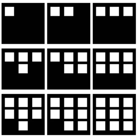
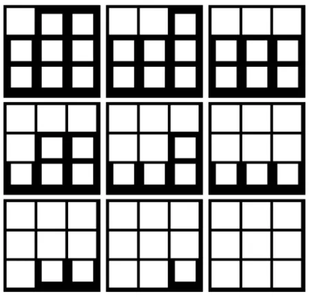
3.2 Object added to image . . . 62

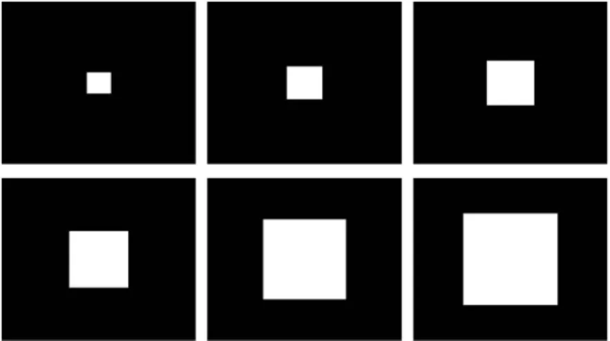
3.3 Objects increasing in size . . . 63

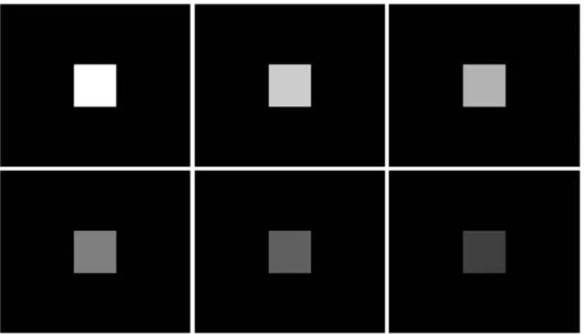
3.5 Object with varied light intensity . . . 65

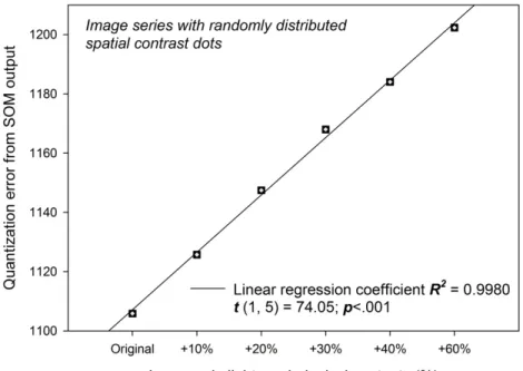
3.6 SOM-QE vs extent of contrast . . . 68

3.7 SOM-QE vs number of objects . . . 69

3.8 SOM-QE vs object size . . . 70

3.9 SOM-QE vs contrast area . . . 71

3.10 SOM-QE vs contrast intensity . . . 72

3.11 Paired random-dot images . . . 77

3.12 Average hit rate . . . 82

3.13 SOM-QE vs dot size . . . 86

3.14 Image dataset used by Pohl et al. [2011a] . . . 88

3.15 Images with local ’lesions’ . . . 96

3.16 Real medical images . . . 98

3.17 SOM-QE on real images . . . 99

3.18 SOM-QE on images with 1 ’lesion’ and with 2 ’lesions’ . . . 100

3.19 Images with global ’lesions’ . . . 101

3.21 Las Vegas photos . . . 114

3.22 SOM-QE on Las Vegas city . . . 116

3.23 Visitors in Las Vegas city . . . 118

3.24 Visitors in Las Vegas . . . 119

3.25 SOM-QE vs number of visitors . . . 121

3.26 SOM-QE vs population trend in Las Vegas . . . 122

3.27 SOM-QE on Las Vegas image series . . . 123

3.28 Water levels in Lake Mead . . . 125

3.30 SOM-QE on Las Vegas Residential North . . . 127

3.31 Population trend in Residential North . . . 128

3.32 SOM-QE vs the Residential North population . . . 129

3.33 Regions of change/no change detected by SOM-QE . . . 131

3.34 SOM-QE dataset for prediction . . . 133

3.35 SOM-QE values: current vs previous . . . 134

3.36 SOM-QE prediction . . . 137

3.38 New and old methods of QE determination . . . 150

3.39 Changes detected by the two methods . . . 151

3.29 SOM-QE vs Lake Mead water levels . . . 153

I.1 R´egions de changement/aucun changement d´etect´e par SOM-QE . 234

I.2 Exemples d’images provenant de l’ensemble de donn´ees de d´etection des changements difficiles `a d´etecter . . . 238

I.3 Nouvelles et anciennes m´ethodes de d´etermination de l’QE . . . . 243

I.4 Changements d´etect´es par les deux m´ethodes . . . 244

I.5 Regions of change/no change detected by SOM-QE . . . 261

I.6 Sample images from the challenging change detection dataset . . . 265

I.7 New and old methods of QE determination . . . 269

List of Tables

3.1 Novice response rate for 5 percent change . . . 80

3.2 Novice response rate for 10 percent change . . . 80

3.3 Novice response rate for 30 percent change . . . 81

3.4 Expert response rate for 5 percent change . . . 83

3.5 Expert response rate for 10 percent change . . . 84

3.6 Expert response rate for 30 percent change . . . 84

3.7 SOM-QE on dataset by Pohl et al. [2011a] . . . 88

3.8 SOM-QE on Berlin and Strasbourg changes . . . 107

3.9 Sampled SOM-QE values of regions in Residential North . . . 130

3.10 Predicted versus actual observation . . . 138

I.1 Sampled SOM-QE valeurs des r´egions dans le Nord r´esidentiel . . 233

Chapter 1

Introduction

Radiologists use time-series of medical images to monitor a patient’s condition. They compare information gleaned from sequences of images to gain insight on progression or remission of the lesions, thus evaluating the progress of a patient’s condition or response to therapy. Visual methods of determining differences be-tween one series of images to another can be subjective or fail to detect very small differences. Similarly, city administrators, planners and politician, among others, require to monitor infrastructure distribution within their cities and determine the changes in city status with time. They need to know the effects of resources, for instance road networks, on the residents’ lives in the different parts of the city. In this thesis, the application of SOM-QE technique to assist the radiologist and the city managers to mine information from an image at a particular time and there-after, monitor subsequent changes occurring with time in the patient and in the

city is demonstrated. Medical images and satellite images are directly analysed to eliminate intermediate procedural bias and to produce fast results.

The concept behind the SOM-QE approach is that through use of images, deter-mination of a scene’s current status is performed and from subsequent images of the same scene, changes that have occurred in time within the scene can be anal-ysed. In this chapter, an overview of the use of artificial intelligence systems to process images and in particular, to detect changes through images is given. The objectives of the research and the specific area of study are also spelt out to give a perspective of the thesis.

1.1

Application of Artificial Intelligence on Images

An image refers to a 2D light intensity function f(x,y), where (x,y) denote spatial coordinates and the value of f at any point (x,y) is proportional to the bright-ness or gray levels of the image at that point. Cameras can capture objects into digital images, providing an avenue for manipulation and study of objects in a computer since the image, f(x,y), has been discretized both in spatial coordinates and brightness. Images are widely used to represent real objects, for example in medical field, images are used to study state of internal body organs. Thus, images provide a ready chance to process a scene data for autonomous machine percep-tion. There exist advance procedures for extracting information from images in a form suitable for computer processing. When in the computer, mostly in form

of arrays, the information can be processed and be put to use in areas such as in character recognition, industrial machine vision for product assembly and inspec-tion, military recognizance, automatic recognition of fingerprints and such similar applications.

Major procedures involved in image processing include

1. image acquisition – the capturing or collection of images,

2. image preprocessing – improving the image in ways that increase the chances of success of next processes,

3. image representation – to convert the input data to a form suitable for com-puter processing,

4. image description – to extract features that result in some quantitative infor-mation of interest or features that are basic for differentiating one class of objects from another and

5. image interpretation which is assigning meaning to an ensemble of recog-nized objects.

Thus, images provide a route for real objects to be analysed and studied in the field of artificial intelligence (AI). The images provide alternatives to other methods of learning the objects like directly measuring quantities/elements in the object – such as temperature of a patient, carbon dioxide concentration in air, composition of soil, among others.

A common technique used to formulate AI systems is the use of artificial neural networks (ANNs). An ANN is made up of several nodes, linked together and whose functioning imitate that of biological neurons of human brain. A node takes input data, performs simple operations on the data and passes the results to other nodes, hence forming a network system of processing nodes. The output at each node, called its activation or node value, can be altered through weight values associated with the link between nodes, a process called learning. During learning, weight values in the nodes are compared to the input value and together with a predetermined learning parameter the amount of change to be effected is calculated. Thus, as P. R. Oliveira and R. F. Romero [1996] puts it, ANN models are specified by the network topology, node characteristics and training or learn-ing rules. The learnlearn-ing rules specify an initial set of weights and indicate how weights should be adapted during training to improve performance. An important property of an ANN is the ability to learn from its environment and to improve its performance through learning. ANN learns about its environment through an iterative process of adjustments applied to its synaptic weights.

There are two major learning strategies that can be employed by an ANN: the supervised learning and the unsupervised learning. In supervised learning, the re-sults given by an ANN are compared with the expected rere-sults and the network makes adjustments based on the errors determined. The goal is to approximate a mapping function of the input to the output so that when new input data is pro-vided, its corresponding output can be predicted. This is the case, for instance, in

pattern recognition. In unsupervised learning, the ANN is provided with the input data and not the expected output. It aims at modelling the underlying structure or distribution of data in order to learn more about the data. In this regard, an ANN algorithm is set up, provided with input data and left on its own to discover and present the interesting structure in the data. Among the techniques in this category of ANN is the K-means clustering algorithm and the focus of this thesis: the SOM algorithm.

Back in 1993, Pal and Pal [1993] predicted that ANNs would become widely ap-plied in image processing and according to Egmont-Petersen et al. [2002], this prediction turned out to be right. ANN applications have been developed to solve different problems in image processing, with strengths and weaknesses being ob-served on each application. These applications have been deployed to solve var-ious problems as categorized in Egmont-Petersen et al. [2002]. For example, in image reconstruction problems, quite complex computations are required and a unique approach is needed for each application. In Adler and Guardo [1994], an ADALINE (an early single-layer artificial neural network and the name of the physical device that implemented this network) network is trained to perform an electrical impedance tomography (EIT) reconstruction. In image restoration problems one wants to derive an image that is not distorted by the (physical) mea-surement system. The system might introduce noise, motion blur, out-of-focus blur, distortion caused by low resolution, among other distortions. Restoration can employ all information about the nature of the distortions introduced by the

system, for example, the point spread function.

Another category of image processing is the image enhancement problems, where the goal of the ANN is to amplify specific features, with most applications being based on regression ANNs. A well known enhancement problem is edge detec-tion. A straightforward application of regression feed-forward ANNs, trained to behave like edge detection, was reported by Griffiths [1988].

In data reduction problems, ANNs are applied in image compression and feature extraction. ANN approaches have to compete with well-established compression techniques such as JPEG, a standard reference in this domain P. R. Oliveira and R. F. Romero [1996]. The major advantage of ANNs over JPEG is that their parameters are adaptable, which may give better compression rates when trained for specific image material. For instance, P. R. Oliveira and R. F. Romero [1996] performed a comparative study and confirmed the performance of the PCA ANN as superior to the JPEG for all the compression ratios used to compress the images in their experiments.

In image segmentation, the image is partitioned into parts that are coherent ac-cording to some criterion. This may be applied as a classification task where labels are assigned to individual pixels or voxels.

In object recognition, locating the positions, possible orientations and scales of instances of objects in an image are done. Egmont-Petersen et al. [2002], has reported several pixel-based and feature-based object recognition applications of

ANNs. Another area in image processing that ANNs are applied is image un-derstanding which combines techniques from segmentation or object recognition with knowledge of the expected image content. This can then be applied, for in-stance, to classify objects such as chromosomes from extracted structures or to classify ships recognized from pixel data, Egmont-Petersen et al. [2002].

More recently, D. Jiang [2013] has applied a SOM based procedure for MRI im-age processing. They noted that MRI imim-ages are usually corrupted by Rician noise that is generated during the image formation. Rician is a non-additive, sig-nal dependent and highly non-linear noise that is difficult to separate from the signal. The SOM algorithm was applied, taking the Rician noise into considera-tion, to de-noise and segment an MRI image. In image segmentaconsidera-tion, an ensemble - a learning paradigm where multiple neural networks are jointly used to solve a problem - of SOMs, Jiang and Zhou [2004], is used to perform segmentation. In, Chen et al. [2017], a SOM is used to develop a crack recognition model for bridge inspection.

1.2

Review of change detection work

Change detection is an important domain in computer vision with applications ranging from video surveillance and medical imaging to remote sensing in urban and environmental change detection. Before changes can be detected, images are typically preprocessed to register them geometrically and correct for any

radio-metric variation Radke et al. [2005a]. In remote sensing, where the goal is to detect urban changes such as the extent of urbanization from a series of 2D map built from satellite images, parallax effects are negligible and synthetic aperture radar is frequently used to lessen the effect of atmospheric and lighting change across time. However, medical images require pixel-accurate registration as a starting point since the situations of their capture are different from that of the satellite images.

Change detection methods can be classified into several categories depending on type of scene, changes to detect, methods, and available information, Sakurada and Okatani [2015]. In 2D image domain, which according to Radke et al. [2005a] , forms a majority of the work they surveyed, a typical approach involve identi-fying a scene, the region of interest (ROI), capture a set of its images at different times, and train an ANN to determine changes between the images. Then a newly captured query image can be run on the ANN to detect changes. A concern in this type of studies is dealing with irrelevant changes such as difference in illumina-tion. It usually requires the images to be captured from the same viewpoint, and thus cannot deal with query images captured from different viewpoints. SOM-QE falls under this category and it requires the query image to be brought into sim-ilar conditions as those of the training image through appropriate preprocessing procedures.

Image science has proposed methods for the automated processing of medical images, which involve various image processing techniques to identify specific

diagnostic ROI and features, such as lesions. Challenges still abound and advance techniques are required to tackle them. For instance, a simple difference map of two longitudinal co-registered MRI volumes fails to detect specific tumour evolu-tion, due to non-linear contrast change between the two data sets, according to An-gelini et al. [2007]. They proposed a computational framework to enable compar-ison of MRI volumes based on gray-scale normalization to determine quantitative tumour growth between successive time intervals. Angelini et al. [2010] proposed three tumour growth indices, namely; volume, maximum radius and spherical ra-dius. The approach, however, requires an initial manual segmentation of images, which can be a time-consuming task. In Konukoglu et al. [2008], they first semi-automatically segmented a tumour in an initial patient scan and then aligned the successive scans using a hierarchical registration scheme to measure growth or shrinkage from the images. This method relies on accurate segmentation and re-quires manual supervision, in order to detect changes of up to a few voxels in the pathology. Pohl et al. [2011a] describe a procedure aimed for difficult-to-detect brain tumour changes. The approach combines input from a medical expert with a computational technique. In this thesis, a new technique is proposed based on self-organized mapping that considers the whole medical image, as opposed to an image segment, as a ROI. This excludes manual benchmarking tasks designed to eliminate inclusion of structures with similarity to tumour pathology. The basic principle behind direct image analysis is that there exists an intrinsic relationship between medical images and their clinical measurements, which can be exploited to eliminate intermediate procedures in image analysis. Compared to traditional

methods, direct methods have more clinical significance by targeting the final outcome. Thus, direct methods not only reduce high computational costs, but also avoid errors induced by any intermediate operations. Direct methods also serve as a bridge between emerging machine learning algorithms and clinical image measurements.

As observed in Radke et al. [2005a], the goal of change detection is to identify the set of pixels that are significantly different between the last image in a sequence and the previous images. But significantly different may vary from application to another, making it difficulty to compare results. SOM-QE technique takes each input feature vector from the image, labels it, and then uses the label to monitor changes that have occurred within the same vector with time. By detecting dif-ference at the input sample level, the technique is able to tell when changes have occurred or not occurred in parts of the image and by extension, changes within regions and sub-regions of an area can be quantified.

Image pairs taken at different times may have temporal differences in illumination and photographing conditions. In Sakurada and Okatani [2015], they had to cope with visual difference in camera viewpoints for the two images as they were cap-tured from a vehicle, although running on the same street and had been matched using GPS data.

To cope with these issues, some of the previous studies consider the problem in the 3D domain. In this domain, Crispell et al. [2012], Huertas and Nevatla [1998], Eden and Cooper [2008], and Taneja et al. [2011] , a model of the target scene is

built to a ‘steady state,’ and used to compared a query image against it to detect changes. The 3D model of the scene is created using a 3D sensor. In Huertas and Nevatla [1998], to estimate the existence of a building, the edges extracted from its aerial images are matched with the projection of its 3D model to detect change. Schindler and Dellaert [2010] proposed using a large number of images of a city taken over several decades. Their method performs several types of temporal in-ferences, such as estimating the time when each building was constructed. More recently Matzen and Snavely [2014] did similar work only that their method uses Internet photo collections to detect 2D changes of a scene, such as changes of advertisements’ billboards and painting on a building’s wall. Work in this domain assume that a 3D model of a scene is given beforehand or can be created from images, and that the input images can be registered to the model with pixel-level accuracy Matzen and Snavely [2014], Schindler and Dellaert [2010] and Taneja et al. [2013]. However, a 3D model is not always available for every city. Be-sides, it is sometimes hard to perform precise image registration, due to lack of sufficient visual features. These are particularly the case when the scene under-goes enormous amount of changes. Working in 3D domain tends to require large computational cost, which can be another difficulty when detection of changes for a large city is required. In the present SOM-QE idea, satellite images, captured from a fixed position, are used and hence avoid the visual problem. In Sakurada and Okatani [2015], they used a method that uses features of convolution neural network (CNN) in combination with super-pixel segmentation. They observed that though CNN features detect the occurrence of scene changes, it did not

pro-vide precise segmentation boundaries of the changes, hence the application of super-pixel segmentation. Therefore, despite having reasonable performance, the method relies on super-pixel regularization and sky/ground segmentation to delin-eate changes accurately.

The work by Sakurada et al. [2013] defines a probabilistic framework in which changes over all possible disparities are evaluated and integrated for each re-projected ray. While this avoids the need for explicit modelling and additional information or sensors, their framework makes the assumption of per-pixel in-dependence in order to be tractable but still remains computationally expensive. SOM-QE is a computationally efficient approach which works from image data to determine variability in the image irrespective of the structure of objects in the image. After the image sequences have been aligned through registration and nor-malized when need be, a similarity measure, the QE, is calculated and employed to determine changes of interest between the data while ignoring other nuisance changes. The definition of what constitutes a change of interest or a nuisance change varies depending on the task. Changes of interest may be purely geomet-ric, such as the appearance or disappearance of urban structures Sakurada et al. [2013], Taneja et al. [2011] and Taneja et al. [2013], or textural, such as changes in billboards or shop-fronts Matzen and Snavely [2014] or surface defects Stent [2015]. Nuisance changes may include lighting effects, for example, cast shad-ows. Stent [2015] proposes training change detection networks from scratch on image patches to classify changes for industrial inspection. In contrast to these

prior works, SOM-QE adopts the self-organizing network approach, first used in Kohonen [1981a] , and demonstrate its ability to learn appropriate, spatially and precise differences between images.

In their review of change detection algorithms, Skifstad and Jain [1989] reported that besides the specific technique used for measuring changes, the change detec-tion process employed in the works they reviewed was generally the same. The input images are first divided up into defined regions. In SOM-QE technique pro-posed here, the image is considered as a whole. This avoids segmentation which can be computationally expensive, depends on some human operator decisions, or is not suitable to some type of land shapes. As pointed out in Palanivel and Duraisamy [2012], uncertain nature is present in the image segmentation process. SOM-QE method assigns a QE value to each input feature vector of an image based on a trained SOM, providing a clear indication on how far the best match-ing unit is from the input vector it won durmatch-ing the learnmatch-ing process.

Most existing change detection methods require a decision as to where to place threshold boundaries in order to separate areas of change from those of no change, Singh [1989]. The threshold value is supplied empirically or statistically by the analyst, rendering the results obtained to be subjective. However, with SOM-QE technique, no thresholding value is required and input feature vectors are treated equally and with the same weight to arrive at the final decision.

Another approach to determining the changes that have taken place between im-ages involve determining changes in land-use zones’ size within cities over time.

Major land uses in a city - built-up, agricultural, water body, undeveloped land, among others are identified. By use of satellite images of the city, plus informa-tion from local city authorities, and/or collecting locally relevant data, the size of each land-use zone is determined. This size is compared for a series of im-ages taken from the ROI over time to determine the change, given as percentage occupation of each land-use item. Conclusions are then derived on changes that have occurred, and the land-use zone that has ‘encroached’ on the other within the specified period is shown, as in Hegazy and Kaloop [2015], Kayet and Pathak [2015] among others.

But there are other causes of changes in cities. Changes in city growth are not limited to the changing size occupied by land-use zones. For example, a new house built within a land-use zone does not cause change in the size of the area, and hence such change will not be captured by the method. Besides, it has been shown that, within a particular land-use zone, features of the other land-use zones occupy substantial land. As determined in Angel et al. [2016], the share of built-up area occbuilt-upied by roads and avenues was on average at 20 ± 2 in 38 cities across the world, as at the year 2015. Thus, SOM-QE method suggested here is able to sense small changes, caused by other factors in addition to those caused by the changing occupational size of a land-use zone. This is done fast enough and can be appropriate for use in an ideal application scenario. It took less than 3 minutes to determine changes between images in a series of 25 images covering the 25 years studied for a ROI in Las Vegas city, USA.

1.3

Motivation for this work

Guthmann et al. [2005] established that shorter return visit interval (RVI) for pa-tient has a positive correlation with percentage change in blood pressure and that RVI may be a tool in the management of hypertension. Schectman et al. [2005] concurs that prolonging the RVI may affect quality of care when prevention mea-sures and chronic disease management receive less attention as clinic visits be-come less frequent.

Schwartz et al. [1999] noted that physicians lengthened revisit intervals for routine visits and shortened them when the visit required a change in the disease manage-ment. On the other hand, changes that have occurred between shortened RVI may be too small to be detected by human observers. There is therefore, a need to have a tool that will enable the automatic detection of subtle but significant changes in time series of images likely to reflect growing or receding lesions.

Likewise, from satellite images, comparing the status of two cities requires the capture of minute details in each, which SOM-QE does effectively. The motiva-tion behind this study is to develop a change detecmotiva-tion method that can be used for visualization of healing or worsening disease condition as captured by medical images or city urbanization or environmental changes as captured through satel-lite images, as well as for the purpose of quantifying the change occurring within time.

1.4

Objectives of the study

The goals of this thesis are threefold:

1. To develop a platform for

(a) determining the variation status of an object through studying the ob-ject’s image at a particular time.

(b) tracking changes taking place in the object over time through images taken from the same object at different times.

2. The platform should be fast enough and appropriate for use in an ideal appli-cation scenario, for example, during a patient’s clinical visit at the hospital.

3. To develop a new method for calculating quantization error in a time series image dataset that is more accurate than the existing method.

The goals are attained by accomplishing the following specific objectives:

1. Analyse objects through their images taken for medical diagnosis, environ-mental monitoring or for city development purposes

2. Assign unique labels to objects through their images based on the object’s contents

3. Differentiate the content of an object at different times based on the object’s SOM-QE values at the different times

4. Detect changes in an object given its series of images taken at different times.

5. Quantify change and give direction of change within an object over time.

6. Quantify variation within an object through studying its images.

7. Develop a robust and fast application for change detection.

8. Provide data for use in change prediction for a region.

1.5

Statement of the problem

Cancer patients require that their condition be monitored seamlessly, with accu-racy, and that they be aware and be informed of the outcomes and their status promptly at every clinical visit. City residents and administrators expect equal de-velopment and distributions of city resources within the city, easy status compar-ison with peer cities and monitoring of the environment for example, for harmful gases, and that they instantly be made aware whenever slight positive or negative changes occur.

Today there is too many late diagnoses of cancer and other chronic diseases that results in too many deaths. There is uneven city development and increase in environmental degradation that has seen the weather pattern changed with unfair and negative consequence for life. If these problems are ignored; deaths will

increase and resources to handle the cascading problems will need to be increased too, the cities may end up being unevenly and skewed developed which could result in feelings of inequality, discrimination, lawsuits and further damage to the leadership ability to guide growths within cities.

SOM-QE is designed to detect small changes that have occurred within a patient, thus reducing periods between clinical visits, senses regional development status and detect minute environmental changes from the relevant images to improve on monitoring of patients and city’s status, and thus solve the problem.

In SOM-QE, a clear path to change detection is set: SOM learns the image to provide its ideal pixel values. Then QE provides the difference between the real and the ideal values, which for different images within a series can tell when changes have occurred in the organ or in the city with time.

1.6

Scope

SOM-QE relies on information it gleans from medical and satellite images in-dividually or/and in the time series image dataset to determine variability and changes in objects as portrayed through their input features. The learning process of SOM determines the set of vectors that acts as the platform on which input vec-tors are referenced to determine their QE values. Hence, the accuracy of the QE value returned relies on this set of vectors. SOM-QE works better when the input

vectors have values of between 0 and 1. It should be noted that manual inspec-tion of scenes can pick up other changes that the current SOM-QE system cannot detect, such as lesions occluded behind internal body parts or a new construction appearing just outside of an existing building that obscures its view. In its present state, SOM-QE takes 2D images as input. 3D images are outside its scope.

1.7

Assumptions

For images to be compared in the proposed SOM-QE algorithm, they must have been captured under similar lighting, colour and orientation conditions. Medical images, satellite images and Urban Atlas maps are assumed to be preprocessed accordingly for effective determination of their SOM-QE values.

1.8

Limitations

SOM-QE uses medical images as provided by radiologist and spatial images from the available satellites. Though sufficient preprocessing procedures are carried out on the images, it is beyond SOM-QE algorithm’s mandate to capture the image in the desired quality. The findings in this research are still valid and useful despite this limitation.

1.9

Thesis organization

After a general overview of SOM, its functional principles and the derivation of QE, the thesis sets out to explain the details behind the SOM-QE concept and states the hypothesis in chapter 2. In chapter 3, a series of application scenarios are described before giving an in-depth description of experiments conducted with human observers on detection of change within images in a ”man versus machine” style. Then, discussion on SOM-QE’s performance on real medical and satellite images is presented. Later, it is shown that SOM-QE values from a time series set of images, can be used to generate predictions on changes in the ROI. The technique is then evaluated, before a new method of determining QE is introduced. In chapter 4, the results of SOM-QE performance in various change detection applications are discussed. Finally, in chapter 5, conclusions on the major findings of the research are presented and their contribution to knowledge is highlighted.

In this chapter, the use of images in computer systems to analyse objects is dis-cussed. Details on the analysis of change that has occurred in an object between two times are provided as they exist in literature, alongside those of the proposed method. In the next chapter, the structure and the working of the new method are explained and demonstrated.

Chapter 2

Self-Organizing Map and the

Quantization Error (SOM-QE)

The new measure of image variation and change detection proposed in this thesis and referred to as SOM-QE, is discussed in details in this chapter. It involves two concepts; the self-organizing map (SOM) and the quantization error (QE). QE is obtained when the final weights of SOM are subtracted from the original input vectors of the image, effectively telling how close the SOM is to the image. To fully comprehend the idea behind SOM and hence SOM-QE, it is important to trace its origin, which is the working of the human brain. This also justifies the choice of SOM over other ANNs in solving the problem of determining variation within objects through their images. Then, details on the design of SOM-QE algo-rithm are presented. Later, the SOM-QE idea is analysed using two basic images

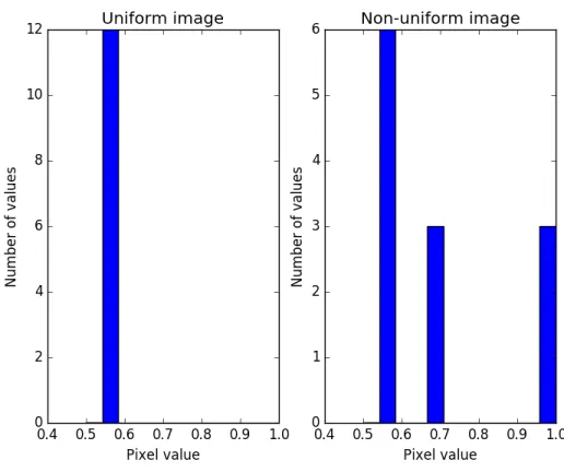
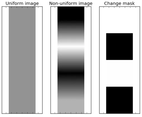
and validated separately using two commonly used dataset content measures – the variance and the histogram. The chapter ends by stating the hypothesis that guides the remaining chapters of the thesis.

2.1

Brain maps and vector quantization

According to Kohonen [2013], for many years it had been known that various cor-tical areas of the brain are specialized to process different modalities of cognitive functions. This was confirmed when Mountcastle [1957] and Hubel and Wiesel [1962] discovered that indeed certain single neural cells in the brain respond se-lectively to some specific sensory stimuli. These cells, called brain maps, often form local assemblies, in which their topographic location corresponds to some feature value of a specific stimulus in an orderly fashion.

Since the brain is an efficient processor of information, it is worth imitating it for an ANN to post reliable results. Image scene, like the ones in medical or satellite images, are composed of various objects which require to be processed separately, or locally, as the brain maps do. For instance, within a lung image there may be a lesion or a water dam in a city map, each of which is processed by a suitable brain map. ANN units can be set to process data in a near-similar manner to the brain maps.

brain maps, at least their fine structures and feature scales, were found to de-pend on sensory experiences and other occurrences. Studies of brain maps that are strongly modified by experiences were reported by Merzenich et al. [1983], among others. In the 1970s, Grossberg [1976], Nass and Cooper [1975] and Perez et al. [1975] investigated whether feature-sensitive cells could be formed automatically in artificial systems through learning.

These works were among the first to succeed in showing that input-driven self-organization was possible. Feature-sensitive units were implemented through competitive learning ANNs. In general, the ANNs had subsets of their units adapt to different input signals during the training process.

However, these early biologically-inspired brain maps were not suitable for practi-cal data analysis. First, they produced partitioned maps after the learning process. The maps were made up of small patches, and there was no global order over the whole map. But, in particular, Suga and O’Neill [1979], TUNTURI [1950]-Tunturi [1952] and Zeki [1980] have shown that brain maps of tonotopic maps, the colour maps and the sonar-echo maps respectively are globally organized, con-firming the first failure of the early brain maps. The second shortcoming of these models was lack of ability to scale up as they could not be used for large networks and high signal dimensionality, even with increased computing power, Kohonen [2013].

SOM introduced a control factor whose amount depends on local signal activity, but which does not contribute to the signals. The control factor plays the role

of determining how much the signal can modify the selected subsets of neural connections in the network. This allows the ANN to work up to the capacity limit of the modern computers.

Then to follow up on improvement of the brain maps, optimally tuned feature-sensitive filters that employed competitive learning, called vector quantization (VQ), were implemented by LLOYD [1982] and Forgy, E.W. [1965] in scalar and vector forms respectively. VQ is currently a standard technology in digital signal processing.

In VQ, feature vectors are partitioned into a finite number of contiguous regions, each represented by one unit vector, called codebook vector. ‘The codebook vec-tors are constructed such that the mean distance, measured in some metric, of an input data item from the best-matching codebook vector, called the winner, is minimized. That is, the mean quantization error is minimized.’,Kohonen [2013].

For simplicity, the VQ is illustrated using the Euclidean distance metric only. Let the input data items constitute n-dimensional Euclidean vectors, denoted by x. Let the codebook vectors be denoted by mi, and mc be a particular codebook vector called the winner as it has the smallest Euclidean distance from x:

mc= argmin i

If p(x) is the probability density of x, the mean quantization error E is defined as:

E = Z

v

||x − mi||2P(x)dV (2.2)

where dV is a two-dimensional differential of the data space V. The objective function E, being an energy function , can be minimized by a gradient-descent procedure.

When input data items are finite, batch computation VQ can be implemented in what is sometimes called Lloyd-Forgy, after LLOYD [1982] and Forgy, E.W. [1965] , and commonly called the k-means clustering.

2.2

SOM

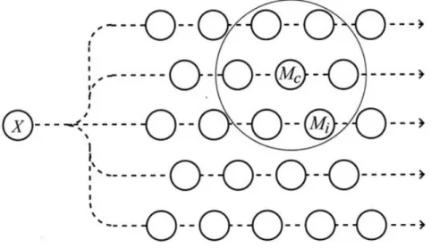
SOM is an ANN that is a non-linear mapping and which is similar to the VQ, except that its processing units become spatially and globally ordered Kohonen [1982]. SOM units are associated with the nodes of a regular, usually 2D grid as shown in Figure 2.1.

Figure 2.1: An illustration of a Self-Organizing Map. An input data item X is broadcast to a set of models Mi, of which Mcmatches best with X. All models

that lie in the neighbourhood (larger circle) of Mc in the array will be updated

together in a training step to make them match better with X than with the rest at the end of the step. Figure courtesy of Kohonen [2014b]

According to SOM founder in Kohonen [2013], the learning principles and math-ematics of SOM are based on a central idea, that; every input data item selects a unit from the map that it matches best. Then, the selected unit and a subset of its spatial neighbours in the map, are modified to match the input vector better.

In effect, SOM learns from a given dataset to produce results that:

1. place similar data samples together.

neighbours in the original dataset, that is, topology preserving.

This explains the main reason for the choice of SOM for the task of this research, that: unlike in most biologically inspired ANNs, the topographic order in the SOM can always be materialized globally over the whole map. Thus, when a trained SOM is given a new and previously unknown input vector, this input is identified with the best-matching unit in SOM and hence it is classified with the particular unit.

During the learning process, matching by similarity is done between the input data and the initial unit values in SOM. Both the input data and the SOM unit values are expressed as real vectors, consisting of numerical results. The vectors are placed on the same scale, through normalization of both scales, in this case by having their maximum and minimum become the same. After that, the standard Euclidean measure is used to determine the level of similarity between the input vector and the map unit vector. SOM has been known to work with even com-plex interdependencies of variables and return results by using Euclidean distance with normalization, Kohonen [2013]. Another consideration made is the presen-tation of an image as an input vector. Images have natural variations caused by translations, rotations, differences in size or in lighting conditions. To minimize the effect of these variation, image registration and normalization are done. Red-green-blue, (RGB), colour as a characteristic feature of the image, is extracted and presented as input vector of the image. This enables the input object to be a restricted set of invariant features, which drastically reduce the computing load,

Kohonen [2013].

The ANN’s learning procedure is unsupervised with specific self-organizing dy-namics that do not require error correction as do supervised learning algorithms. SOM produces a lower-dimension representation of the input space and for each input vector, a competitive winner-take-all learning algorithm Kohonen [1981a] achieves the lower-dimension visualization of the input data. SOMs are typically applied as feature clustering of input data starting from an initially random feature map. The input data are recursively fed into the learning procedure to optimize the final map into a stable representation of features and ROI. Each region of the map can be considered in terms of a specific feature class of the input space. Whenever the synaptic weights associated with a node of the map match the input vector, that specific map area is selectively optimized, bringing it closer in resemblance to the data of the class the input vector belongs to. From an initial distribution of random weights and over thousands of iterations, SOM progressively sets up a map of sta-ble representations of image regions or ROI. Each corresponding region of the final map is a feature cluster and the graphical output is a certain type of feature map of the input space.

The map structure obtained from the learning process leads to SOM being viewed as a topology preserving transformation from high dimensional space to a low dimensional space Kohonen [1995]. This low dimensional space is usually a 2D or 1D grid. From this point of view SOM can be compared to other dimension-ality reduction and data unfolding methods, Moosavi [2014]. Among the

meth-ods, which are rooted in Topological Data Analysis (TDA), Zomorodian [2011], are; Multidimensional Scaling (MDS),Kruskal [1964], Locally Linear Embedding (LLE) Roweis and Saul [2000], ISOMAP Tenenbaum [2000], and Mapper Singh et al. [2007]. But SOM goes beyond this. Besides the transformation of data, SOM discovers ‘the shape of data’ in terms of topology and geometry, which leads to successful methods in visualization and exploratory data analysis tasks. In this view of SOM, regardless of the global dimensionality of the observed data set, given a similarity measure among individual data points, a self-referential co-ordinate system can be constructed, by which each instance of the observation becomes a dimension for itself compared to all the other points, Moosavi [2014].

Topology preservation implies that vectors that are close in the high-dimensional space end up being mapped to nodes that are close in the 2D space. For example, lesions in a lung will occupy the same relative position in the trained dataset as they did in the original image, or that a particular building in the city maintains its location relative to other buildings in the original image.

Topological preservation is attained when the BMU and its neighbours ‘learn’, which is accomplished through adjusting their weights to fit more closely to values of an input vector. The ‘learning’ is more for the BMU and decreases as the distance of a neighbouring unit from BMU increases, as explained in details in section 2.4.

These two facts, grouping input samples and topology preservation, makes SOM a good fit for the goal of this thesis. Data is learned and grouped based on its

similarity while considering their current location. This means that each data item makes contribution to the variation in the image from its local location, making the SOM-QE value to be a more reliable and accurate measure of variation.

2.3

SOM learning: winner-takes-all

The vector space of the SOM is Euclidean Kohonen [1981a], and the central idea behind the principles of self-organized mapping is that every input data item is matched to the closest fitting neuron unit of the neural map, the winner. The winning neurons for the corresponding regions are progressively modified on that principle until they optimally match the entire data set. The learning procedure follows the neural-biological principles of lateral inhibition and the general rule of Hebbian synaptic learning Hartline et al. [1956]. On the other hand, since the spatial neighbourhood around the winners in the map are continuously modified during learning, a degree of local and differential ordering of the map is mathemat-ically applied in the smoothing process. The resulting local ordering effect will gradually be propagated across the entire SOM. The parameters in SOM model can be variable and depend on the type of input data being implemented. The goal of this winner-take-all learning is to ensure that the final map stably represents critical similarities in the input data.

In general two operations take place in the SOM learning: first, there is the spatial clustering of activity into one centre of high activity, the location of which is a

function of the input pattern. This location becomes the winner. Secondly, there is the adaptive modification of the interconnections in the local area around the winner such that all neural functions in this area are tuned better to the prevailing input activity and will respond stronger to it. This local area imitates the brain map, as explained in section 2.1.

Thus, for different inputs, different local areas will be modified, and in the long run different areas of the ‘map’ will become selectively tuned to different domains of the input in an ordered and almost optimal fashion.

Figure 2.1, adapted from Kohonen [2013] , shows the effect of input data to the map.

Only a subset of the map units is able to learn the present input vector and even within the subset the amount of learning is varied – strength of learning decreases as the distance to the unit from the BMU increases. Figure 2.2 is a synonymous illustration with the real feeling on human skin. The sensing of the sharp object pressed on the skin is more at the point of touch and reduces outwards from this point. On SOM, the ‘point of touch’ is the BMU while the rest of the region on the skin that will feel the touch by the sharp object corresponds to the BMU’s ‘neighbourhood’.

Figure 2.2: The spatially diffusive local sensitivity of a single touch receptor may be used to illustrate the functional model underlying SOM. On pressing the skin surface with a pointed object, the feeling is more intense at the point of touch and reduces as distance from the point increases outwards.

2.4

Network architecture

A 2D organization of the map units was adapted in this work since it is usually effective for approximation of similarity relations of high-dimensional data, as is the case with images, Kohonen [2013]. Since it is not possible to guess or estimate the exact size of the SOM map beforehand, it was determined by the trial-and-error method after seeing the quality of the first guess, Kohonen [1981b]. For most of the images encountered in this work, a 4 by 4 map, giving 16 processing units, was found to be the optimal size.

form the network.

In the detailed implementation of the original SOM algorithm provided in Buck-land [2005] , each learning unit occupies a specific topological position - an x-y coordinate on the map - and contains a vector of weights of the same dimension as the input vectors. In most of the cases in this thesis, RGB values of the image are extracted and used as input vectors to the map, hence the units are set to have three weights, one for each element of the input vector: red, green and blue.

The adaptation of the synaptic vectors in the models is done as proposed by Ko-honen in KoKo-honen [1981b] and KoKo-honen [2014a]:

1. Determine the best-matching unit for the current input vector.

2. Make the best-matching unit and its topologically nearest neighbours more similar to the input vector.

To attain this, SOM does not need a target output to be specified, instead, where the model weights match the input vector, that area of the map is selectively changed through the learning process to improve its resemblance to the data in the input vector. From an initial distribution of random weights in the units, and after several iterations, the SOM eventually settles into a map of stable zones. Each zone is effectively a feature classifier, such that the graphical output repre-sents feature map of the input space, Figure 2.3. At the end of the training process, if any new, previously unseen input vector is presented to the network, it will stim-ulate units in the zone with whose weight vectors are more similar to its values

than the other zones. This effectively, clusters the new input as a member of the zone it stimulates.

The region around the BMU where units are adjusted at every iteration is identified by the neighbourhood radius. This is a value that starts large, typically set to the ’radius’ of the map, but diminishes at each time-step. This radius, together with the learning rate, determine the amount of learning to be effected on the units.

As illustrated in Buckland [2005], the training steps involved in the SOM algo-rithm are:

1. Each unit’s weights are initialized using vector values picked randomly from the image.

2. A vector is chosen at random from the set of RGB features extracted from the image data and presented to the map.

3. Every map unit is evaluated to determine the amount of difference between its weights’ values and the input vector’s values. The unit with the smallest difference ‘wins’ the input vector to become its BMU.

4. The radius of the neighbourhood of the BMU is calculated. Any unit found within this radius from the BMU is deemed to be inside the BMU’s neigh-bourhood.

5. Weights of units within the BMU’s neighbourhood are adjusted to reduce their difference with the input vector. The closer a unit is to the BMU, the

more its weights are altered, making it ‘learn’ more than the units that are far.

6. steps 2 to 5 are repeated for a specified number of iterations, N.

To know the BMU for the input vector, all the units are iterated as their Euclidean distance with the current input vector is calculated. The Euclidean distance, d, is calculated as: d= v u u t i=n X i=0 (Vi− Wi)2 (2.3)

where V is the current input vector and W is the unit’s weight vector. The unit with the lowest distance becomes the BMU for the input vector.

During each iteration and after the BMU has been determined, units within the BMU’s neighbourhood are identified. These units – they form a local region for the input vector - will have their weight vectors altered in the next step. This optimizing of the region for the input vector, sets SOM aside from other ANNs. To attain this creation of local regions, first the radius of the neighbourhood is calculated then, with the BMU as the centre, the radius is used to cover a circular area around the BMU. This becomes the neighbourhood region. At the beginning of the training, this radius is set at half the map width as in Kohonen [2013].

During learning, the neighbourhood reduces in size over time, effected by the exponential decay function:

σ(t) = σ0exp(

−t

λ ) t= 1, 2, 3... (2.4)

where σ0denotes the width of the map at time t0 and λ denotes a time constant. t

is the current iteration of the loop. The value of λ depends on σ and on the number of iterations the algorithm is set to execute:

λ= N logσ0

(2.5)

N , the number of iterations to be done by the learning algorithm is set by the user at the beginning.

In practice, BMU’s location can be anywhere in the map, depending on the input being processed by the network. With time, the neighbourhood reduces to the size of one unit, the BMU.

With a known radius, all the units are iterated, determining if they are within the radius or not. When a unit is within the neighbourhood, its weight vector is adjusted as follows:

W(t + 1) = W (t) + Θ(t)L(t)(V (t) − W (t)) (2.6)

This is SOM’s learning method, where t is the time step and L is a small variable called the learning rate, which decreases with time. From this equation, the new

adjusted weight for the unit is equal to the old weight (W ), plus a fraction of the difference, (L and θ), between the old weight and the input vector (V ).

The decay of the learning rate is calculated at each iteration using the equation:

L(t) = L0exp(

−t

λ ) t= 1, 2, 3... (2.7)

just like in equation 4, except this time it is the learning rate that decays.

The learning rate at the start of training is set by the user. It then gradually decays over time so that during the last few iterations it is close to zero.

Equation 2.6 incorporates the learning rate decay over time and the learning strength that is proportional to the distance a unit is from the BMU. At the edges of the BMUs neighbourhood, the learning process has very little effect.

Ideally, the amount of learning should fade over time following a Gaussian decay. In equation 2.6, θ represent the amount of influence of a unit’s distance from the BMU on its learning, and is given by:

Θ(t) = exp( −d

2

2σ2_(t)) t= 1, 2, 3... (2.8)

where d is the distance a unit is from the BMU and σ is the width of the neigh-bourhood function as calculated in equation 4. θ also decays with time.

component - red, green and blue, the input vectors are normalized, so that each component has a value between 0 and 1. This is to match the range of the values used for the units’ weights.

SOMs are commonly used in data clustering, abstraction and as visualization aids. They make it easy for humans to see relationships between the vast amounts of data carried in images. In this thesis, a new use of SOM is suggested; that the QE that is derived from SOM can make it easy for humans to see the variations in the vast data within an image.

2.5

The trained SOM: final synaptic weights

Another view of SOM is that of a statistical method of data analysis using an un-supervised learning algorithm whose goal is to determine relevant properties of input data without explicit feedback from expected results. Originally inspired by feature maps in sensory systems as explained earlier, it has greatly contributed to our understanding of principles of self-organization in the brain and the de-velopment of feature maps as observed in Martin and Obermayer [2009]. Koho-nen [1996] points out that although the brain mechanisms are extremely complex and contain many details, the theory of their cognitive abilities must be based on much fewer general principles. This is in line with SOM’s ability to reduce multi-dimensional data to lower-dimension data. Traditionally it has been held that ‘in-telligent’ information processing takes place from signal processing in adaptive

network structures. With a degree of adaptation that is made controllable, SOM is a successful implementation of this principle and can be viewed on different levels of abstraction: as a physiological model, or a simplified numerical algorithm.

Through an interplay of neural principles of lateral inhibition and Hebbian synap-tic learning within a localized region of the one-layered neural network, the SOM acquires a low-dimensional representation of high-dimensional input features that respects topological relationships of the input space. This is progressively achieved through the updating of the initial synaptic weights, using equation 2.6. At the end of learning, when all neurons optimally match the data from the input data set, SOM acquires the matrix of the final synaptic weights. Thus, for different inputs, different local areas will be modified, and in the long run, different areas of the ‘map’ will become selectively tuned to different domains of the input in an ordered and almost optimal fashion, Martin and Obermayer [2009].

The final weights of SOM are the BMUs, each being associated to the input vec-tors it won. A BMU acts like the centroid in VQ to this category of vecvec-tors which are more similar to each other than to those associated to a different BMU. Figure 2.3 shows a trained SOM, with input vectors distributed to the 30 units using the criteria explained in the previous section.

Figure 2.3: An example of a trained SOM. Each BMU is represented by a rect-angular cell on the display. In this particular case, the SOM was a 5 by 6, and it considered four features, the RGBA, from an Urban Atlas map. It was trained for 10 000 iterations at a learning rate of 0.2 and a neighbourhood distance of 0.1. The colour distribution here shows how the samples from the atlas were mapped into the 30 units of the SOM after the training.

Using the colour bar provided in the figure, one can compare the number of input data samples won by each SOM unit. The input samples are made members of the local region with the BMU as their centroid. Effectively, the BMU becomes

the representative of all the samples it won, drastically reducing the dimension of the original data.

The task of SOM in SOM-QE is to create a standard platform on which QE is determined. This standard is composed of a set of 2D vectors, the BMUs, that has been generated through the competitive process described in sections 2.3 and 2.4 above.

Just like in other standards that provide a scale, for instance, to ensure uniformity in the results they post, this set of BMUs ensures that variation within images of a time series is measured and based on a uniform criteria that is capable of being replicated.

In section 3.7, a new method of calculating the QE is suggested that utilizes a fixed BMU for each input sample throughout a time series of images.

2.6

The quantization error (QE)

QE of an image dataset address the question; how well does each BMU fit each of the samples it won? In this section, this question is addressed, taking into consideration QE’s contribution in determining the variation within an image.

The task of finding a suitable subset that describes and represents a larger set of data vectors is called vector quantization, Gray [1984]. SOM quantize data since at the end of the learning process, each BMU has some data samples attached to it.

The BMU can be regarded as the centroid of the group of samples it won. Despite the competition among the units to win over input samples, it is likely that the unit did not become an exact match of the sample. Therefore, even a BMU for an input may still have some differences with the input from the image despite winning it, expressed as:

QE= x − BM U (2.9)

where the BM U is taken from the set of final weights attained by the trained SOM, and x is an input sample it won. QE tells how far the BMU is from the input vector it won during the learning process.

This difference is the core idea that is applied to attain the objectives of this the-sis. Equation 2.9 is the mathematical expression of determination of QE. To be a representative of the entire image, the average QE from each of the image’s input samples is calculated and used as a label for the image. Statistically, the mean of data is a preferred measure of central tendency as it takes into considerations all data points. The mean value gives the lowest amount of error from all other values in the data set each time a measure is taken. The mean QE is given by equation 2.11. Thus, QE measures variation and when determined for each input sample in the image, it provides a measure of variations across the image.

Since each QE value is determined from the final weights of the same trained SOM, the QE values for different images or input vectors can be compared to each other to determine change between them.