The design and implementation of a demonstration supplementary control system

THE DESIGN AND IMPLEMENTATION OF A DEMONSTRATION SUPPLEMENTARY CONTROL SYSTEM

M. Ruane, J. Gruhl, F. Schweppe, B. Green (ERT) and B. Egan (ERT)

MIT Energy Laboratory Report No. MIT-EL 80-033 December 1976

MITLibraries

DISCLAIMER OF QUALITY

Due to the condition of the original material, there are unavoidable flaws in this reproduction. We have made every effort possible to

provide you with the best copy available. If you are dissatisfied with this product and find it unusable, please contact Document Services as soon as possible.

Thank you.

Some pages in the original document contain pictures, graphics, or text that is illegible.

FINAL REPORT

THE ENERGY LABORATORY

MASSACHUSETTS INSTITUTE OF TECHNOLOGY 77 Massachusetts Avenue

Cambridge, Massachusetts 02139

THE DESIGN AND IMPLEMENTATION OF A DEMONSTRATION SUPPLEMENTARY CONTROL SYSTEM

M. Ruane, J. Gruhl, F. Schweppe,

B. Green (ERT) and B. Egan (ERT)

MIT Energy Laboratory Report No. MIT-EL 80-033 December 1976

revised December 1980

Prepared under the support of United States Atomic Energy Commission

Contract No. AT(11-1)-2428

~tYc~---~----"~-;-TABLE OF CONTENTS Page Table of Contents 2 Table of Figures 4 Table of Tables 6 Summary 7

Definitions of Key Terms 9

1.0 Introduction 11

1.1 Motivation 11

1.2 Project Description 12

2.0 System Design 15

2.1 Source Characteristics 15

2.2 Air Quality Monitoring Network 21

2.3 Meteorological Network 23

2.4 Air Quality Model 24

2.4.1 Deterministic Model 24

2.4.2 Downwash Model for Seward 30

2.5 Control Strategy 35

2.5.1 Deterministic Control Strategy 35 2.5.2 Probabilistic Control Strategy 45

3.0 Demonstration Period 55 3.1 Demonstration Approach 55 3.2 Demonstration Results 57 3.3 Conclusions 61 4.0 Background Effects 73 4.1 Data 73

4.2 Mean Concentration Analysis 78

4.3 Peak Concentration Analysis 79

4.4 EPA-Larsen Method 80

4.5 Stochastic Background Modeling Methodology 80 5.0 Air Quality Modeling in Complex Terrain 82 5.1 Shortcomings of the Original Model 82

CONTENTS (2)

Page

6.0 SCS Reliability Analysis 85

6.1 Approach 85

6.2 Results for Demonstration Period Model 87

6.2.1 Two Source vs. Eight Source Analysis 87

6.2.1.1 Choice of Sample Function 87

6.2.1.2 Model Conservatism 88

6.2.1.3 Direct Comparison 90

6.2.2 Sulfur Content Analysis 97

6.2.3 Plant Load Analysis 97

6.2.4 Weather Forecasting Errors 100

6.2.5 Model Errors 110

6.2.6 Total Error Ratio R 110

6.3 Results - Model Modifications 115

6.4 Conclusions 118

7.0 Economic Analysis 121

7.1 General Comments and Results 121

7.2 Technique for Transferability 133

8.0 Future of SCS 136

References 138

Appendix A Mean Concentration Analysis Appendix B Peak Concentration Analysis

Appendix C Calculating Source Reduction by Larson's Method Appendix D Mathematical Background Model

TABLE OF FIGURES Figure Number 1.2.1 2.1.1 2.1.2 2.4.1 2.5.1 2.5.2 2.5.3 3.1.1 3.1.2 3.1.3 3.2.1 3.2.2 3.2.3 3.2.4 6.2.1a 6.2.1b 6.2.2a 6.2.2b 6.2.3a 6.2.3b 6.2.4a 6.2.4b 6.2.5a 6.2.5b 6.2.6a 6.2.6b 6.2.6c 6.2.6d 6.2.7a 6.2.7b 6.2.8a 6.2.8b 6.2.9a 6.2.9b 6.3.1a 6.3.1b 6.3.2a 6.3.2b Title Components of an SCS Chestnut Ridge Area Dispatching Hierarchy

Portion of the Forty by Forty Grid Showing Pollutant Concentrations in Parts per Hundred Million

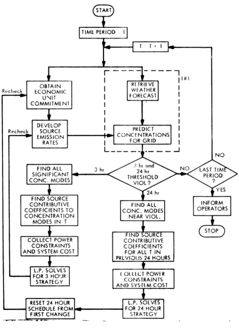
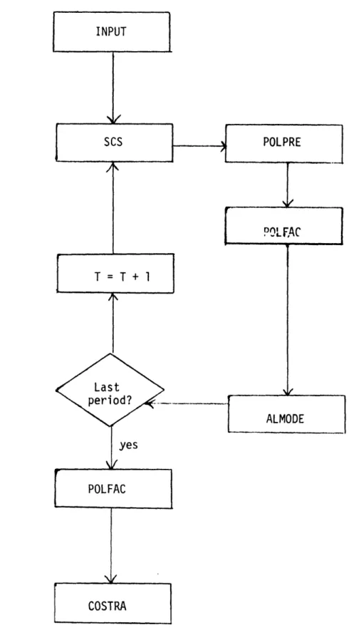
Block Diagram Flowchart of Control Strategy Logic

Flow of Subroutines Used to Determine Optimum SCS Control Strategy

Cumulative Distribution of PCc Demonstration Period Implementation Control Strategies Form - 3/20/76 Data Collection

Seward Output During Control Actions Mobile Van S02 Readings

Control Action Monitoring Seward Monitor Data

Sample Distribution of In8RM - 3 hr. avg.

Sn8_R M - 24 " " ln2RM - 3 " " " 1" In21 M - 24 " " " _{" InRM - 3 " "} " " " InR1 M - 24 " " " " "

lnRS

1nR

Wind Direction Errors " Wind Speed Errors "

" _{" Mixing Depth Errors} "

" _{" Stability Class Errors}

" InR. -" nR -" InRM -" nR -" InR -l" nR" -" InR-" -" ln8 R*M-" ln 8 R*M-3 hr. 24 " 3 " 24 " 3 " 24 " 3 " 24 " 3 " 24 " avg. I I 'I I' II II II I I Page 13 17 19 34 39 41 48 56 58 59 69 70 71 72 91 92 93 94 95 96 98 99 101 102 103 104 105 106 108 109 111 112 113 114 116 117 119 120

FIGURES (2)

Figure Number Title _Page

7.1.1 _{Comparison of predicted 3 hour 122}

pollutant concentration and monitored levels

7.1.2 _{Comparison of predicted 24 hour 123} pollutant concentrations and monitored

levels

7.1.3 Fraction of unit commitment - Seward 125 7.1.4 Total Control Costs for moving various 127

3 hr. predicted incidents by various amounts

7.1.5 Total Monthly Costs for controlling 128 predicted 3 hr. concentrations down to

various thresholds

7.1.6 Annual costs for controlling predicted 129 3 hr.concentration down to various levels

7.1.7 Six highest 3 hr. predicted concentration 130 levels contributing to 24 hr. predicted

maxima

7.1.8 Distribution of 24 hr. predicted concentrations 131 when the only control is the imposition of

various 3 hr. thresholds

7.1.9 Costs for controlling predicted 24 hr. 132 concentration to 140 ppb

7.2.1 Midwestern Pennsylvania terrain used in 134 air quality model

TABLE OF TABLES

Table Number Title Page

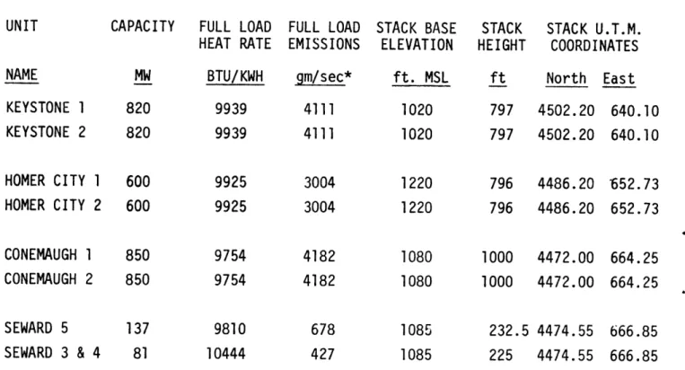
2.1.1 Plant Parameters 18

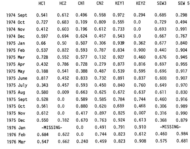
2.1.2 Monthly Availabilities 20

2.2.1 Monitor Locations 22

2.4.1 Terrain Correction Factors for the Stability 29 Classes

2.4.2 Examples of Downwash Concentrations vs. 32

Plant Operating Levels

2.5.1 Utility Scheduling Problems 37

2.5.2 Control Action Comparison 38

2.5.3 Key Factors Affecting Design/Operation 47 and Analysis

2.5.4 Control Strategies Form l-D 50

3.2.1 Control Action Summary 62

3.2.2 Control Report Summary 63

3.2.3 "Grab Sample" Coal Analysis 67

3.2.4 Mobile Van Sampling Data 68

4.1.1 Chestnut Ridge SCS-SO0₂ 24-hr. Running 74 Averages (MAX) PPB

4.1.2 Chestnut Ridge SCS-SO0₂ 3-hr. Running 75 Averages (MAX) PPB

4.1.3 Chestnut Ridge SCS-S02 1-hr. Running 76 Averages (MAX) PPB

4.1.4 Chestnut Ridge SCS - Data Capture 77

SUMMARY

The overall goal of the Chestnut Ridge Supplemental Control System (SCS) demonstration project was to demonstrate how an existing monitoring network, existing air quality models, and existing meteorological forecasting methods could be combined with a new control strategy to integrate SCS into

electric power system operation. This final report covers the period February 1, 1974 to May 31, 1976.

A complete SCS for four power plants in the Chestnut Ridge region of Pennsylvania was implemented. The design is described in Section 2. The demonstration period, discussed in Section 3, showed that it is definitely possible to integrate a sophisticated SCS into electric power systems operation. The basic methods used in this project are felt to be directly extendable to other situations.

The only new technology originally envisioned for this project was the control strategy which decides the power system's response to predicted or potential violations. One of the key problems was the need for the control strategy to ensure that standards are not violated in spite of the presence of uncertainties in predicted ambient concentration levels. As discussed in Section 2.6, the implemented control strategy accounted explicitly for the uncertainties.

The point source air quality model-used during the demonstration period was primarily a state-of-the-art model. However, as discussed in Section 2.5, a relatively new innovation involving downwash modeling was critical to the success of the demonstration.

During the course of the project, a large data base of SO concentrations, meteorological measurements, weather forecasts, and power systim data was established and stored in a manner which was easy to access and manipulate. Studies were done using these data, both before and after the actual demonstra-tion. Some of the methodologies used and developed are applicable to a

variety of problems including many non-SCS types. The results of these studies will now be summarized.

State-of-the-art air quality modeling was not as satisfactory as initially hoped in coping with the rough terrain in the Chestnut Ridge

area. Research on improving point source air quality modeling for rough terrain was successfully undertaken using the data base after the

demonstration period was over. The results are discussed in Section 5 with

details provided in Appendix E.

The Chestnut Ridge area was discovered to have an unexpectedly high background SO level. The data base enabled this background problem to be addressed in %he four ways summarized in Section 4: mean concentration analysis, peak concentration analysis, EPA Larson method, and stochastic

modeling. All four approaches are felt to be applicable in other

concentration. The stochastic modeling appears to be a new methodology with particularly great potential. Details of these four methods are given in Appendixes A, B, C, and D.

Uncertainty arising from air quality modeling errors, weather forecasting errors, fuel sulfur contents, power system economics, and plant availability plays a central role in SCS analysis, design, and implementation. A

systematic analysis methodology was applied to the data base to explore how these various uncertainties propagate through the overall SCS and affect its operation. This work is discussed in Section 6.

The control strategy minimizes cost subject to the constraint that

ambient standards are not violated. Because of the uncertainties, the control strategy operates in a conservative fashion, that is, it often takes control actions that would not be required if the uncertainties did not exist.

The control strategy was applied to the data base to determine how the overall economics behave and how they are affected by the presence of un-certainty. These results are discussed in Section 7.

During the course of the project, opinions were developed on the potentia l future role of SCS. We feel that SCS provides a viable tool for dealing with the energy, economic, environmental crisis. These opinions are discussed in more detail in Section 8.

DEFINITIONS OF KEY TERMS

The key terms used in this document are defined as follows:

Air Quality - Ground-level pollutant concentrations and their temporal and spatial distributions

Air quality Monitoring Network - An array of continuous sampling stations that measure air quality

Air Quality Violation - the occurrence* of an ambient SO2 concen-tration that exceeds an ambient air quality standard for S02 at any point within a designated liability area

Background Study - The collection and analysis of source, me-teorological, and air quality data for the purpose of developing the SCS operational procedures.

Closed-Loop Mode of Operation - The SCS operational mode in which emission control decisions are based upon real-time measurements

by the air quality monitoring network.

Constant Emission Control (CEC) - The continuous limitation of SO emissions from a stack through techniques such as stack gas cl aning or use of low-sulfur fuel

Control Decision - The decision as to what degree to curtail emissions

Controlled Emissions - The SO emission rate resulting from im-plementation of the control dicision

Control Strategy - The sequence of recommended control decisions produced by the operating model for the period of the current forecast

Data Storage - Synchronous records of meteorological data, emission data, dispersion model predictions, control decisions and measured air quality

Dispersion Model - A mathematical model that relates meteorological data, emission rates, other source data and terrain factors to air quality in the vicinity of the source

*Many of these definitions have been taken from (EPA, 1976).

Modi-fications have been made to correspond with the use of these terms in this project.

Effective Stack Height - The sum of (1) the physical stack height above grade and (2) the rise of the plume centerline after leaving the stack. The latter is due to the plume's initial vertical mo-mentum and buoyancy

Emission Monitors - A system for the sampling and recording of SO2 emission rates.

Isolated Source - A source sufficiently remote from other significant sources such that it can and will accept responsibility for attaining and maintaining ambient air quality standards for SO2 within a

desig-nated liability area

National Ambient Air quality Standards (NAAqS) - The primary NAAQS for SO are a 24-hour average concentration of 365 micrograms per cubic Aeter (not to be exceeded more than once per year) and a maxi-mum annual average concentration of 80 micrograms per cubic meter;

the secondary NAAQS for SO2 is a 3-hour concentration of 1300

micro-grams per cubic meter (not to be exceeded more than once a year) Open-Loop Mode of Operation - The SCS operational mode in which

emis-sion control deciemis-sions are based on calculations by the operating

model in conjunction with either real-time or projected meteorologi-cal and emission data

Operating Model - The key element in the open-loop mode of SCS opera-tion consisting of the control model and the dispersion model. The model generates the control strategy using forecasted meteorology

and power system data

Supplementary Control System (SCS) - A system by which SO emissions are curtailed during periods when meteorological conditioNs conducive

to ground-level concentrations in excess of ambient standards for SO₂ either exist or are anticipated

System Upgrade - The continuous and systematic evaluation of the SCS elements and their interrelation in order to improve the reliability of the SCS in maintaining ambient standards for SO₂

Threshold Concentration - A measured or predicted short-term SO con-centration and/or rate of change of concentration that serves ai an

indicator of a potential violation of an ambient SO2 standard

Time Delay - The time elapsed between the emission control decision and the time that the reduction in emissions begins to affect ambient air quality. This delay is equal to the sum of the time required

to achieve the reduced emission level and the time required for the atmospheric transport of the reduced emissions to the point of the maximum ground-level concentration

1.0 INTRODUCTION

1.1 Motivation

The control of sulfur dioxide emissions from large stationary sources has been in the forefront of the national debate on environmental quality and energy supply. Congress, the EPA, the courts, industry and researchers searched for an acceptable trade-off between protecting the public from the effects of SO and using fuel resources containing sulfur. This report

do-cuments a resgarch effort on one part of the overall trade-off question:

using supplementary control systems on electric power plants in complex terrain.

In its entirety, the trade-off question is sufficiently complex to have consumed almost a decade since the 1967 Air Quality Act and 1970 Clean Air Act were passed. For our purposes, the debate can be traced to Congress'

1970 Clean Air Act, which required the EPA to establish standards for the

control of air pollution, and required the states to enact State Implementa-tion Plans (SIP's) to achieve or improve upon the federal standards. Am-bient sulfur dioxide standards were set so as to protect the public health

and welfare (Federal Register, 1971) and the debate was started. Section 110

of the Act requires any SIP for emission control to include emission limi-tations and schedules for compliance "and such other measures as may be necessary to attain and maintain ambient air quality standards." The elec-tric utility industry interpreted this as allowing any technique which would meet this goal. EPA, however, maintained that it was required by

Congress to disapprove any SIP without continuous emission control techniques,

unless such techniques were infeasible.

Continuous emission controls are those which operate all the time. The use of conforming fuel (i.e., fuel whose sulfur content will produce accep-table emissions) is the most common continuous emission control in use. Con-forming fuel can be purchased, blended by a user from "clean" and "dirty" supplies, or made by desulfurizing "dirty" fuel. For many future fossil power plants, most of which must burn coal, conforming fuel supplies will be inadequate. Flue gas desulfurization is the alternative means of con-tinuous emission control for such plants.

The utilities' reluctance to use continuous controls was based on a number of factors, including insufficient availability, costs, reliability problems, and secondary environmental impacts, such as sludge disposal. Much of the trade-off debate has centered on the availability, costs, and relia-bility of the continuous controls. This report does not address those issues directly. Rather, we consider one of the alternatives to continuous controls.

Non-continuous or dynamic emission controls are those which operate only part of the time. Non-continuous emission controls which assist some form of continuous controls are referred to in this document as supplementary control systems (SCS's). Non-continuous controls which are the only

con-trols applied to protect air quality are referred to as intermittent control systems (ICS's).

Supplementary and intermittent control systems both are enacted

whenever the scheduled source emissions (whether controlled or uncontrolled) and expected meteorology will combine so as to threaten ambient standards. Both systems act to protect the standards by reducing emissions until the atmosphere's dispersive ability increases. For ICS, the potential need for control is apparent, since no continuous control is in effect. For SCS, any use of the non-continuous system implies that the continuous system's emission limitations are inadequate.

Under what conditions might this inadequacy of continuous emissions control be expected to occur? At present, the most likely case is when the source plume interacts with complex terrain. A second possibility is when other sources or background concentrations combine with the controlled source to cause a threat to the standards. In the future, as the economy grows and more sources compete for the same air resource, the logic which led to the need for continuous controls will lead to the situation where even con-tinuous controls are inadequate to protect the ambient standards at all times. The alternative of tightening allowable emission limits is a possible solution, but one that runs counter to the need for economic, reliable energy and may be limited by the technologies of continuous controls. In the future, and at present in some special cases, even continuous controls may require sup-plementary help to maintain human health and welfare.

On April 19, 1976, the U.S. Supreme Court declined to hear the Big Rivers case, thereby upholding a lower court's ruling that the EPA is empowered to forbid the use of ICS in any SIP. ICS, as part of the overall trade-off deabte, seems to be a dead issue. The concern over increased atmospheric loadings and suspended sulfate levels has eliminated ICS as a viable compro-mise for sulfur dioxide control.

We believe that SCS is not a dead issue, nor should it be. This report was being prepared at a time when Congress was attempting to clarify its intentions for the Clean Air Act through the Clean Air Act Amendments of 1976

(U.S. Senate, 1976). Although the 93rd Congress adjourned without enacting these

amendments, the Senate Committee Report clearly indicated a preference continuous controls and tended to classify all dynamic controls together

as the same technology. We believe Congress should leave open the possibility of using supplementary control systems, and should make clear the distinction between SCS and ICS. Our experience has shown the necessity of SCS to pro-tect air quality standards.

1.2 Project Description

Our experience has been based on a field demonstration of a supplementary control system. Called the Chestnut Ridge SCS after its location in western Pennsylvania, the system supplemented a continuous emission control scheme using a low-sulfur fuel supply which complied with the Pennsylvania SIP. Our SCS was similar to most SCS designs in that it attempted to take advantage of the atmosphere as a time-varying resource and was based on a combination of several existing technologies: monitoring, forecasting,and control, as shown in Figure 1.2.1.

M

Meteorological _Control 0

I Power

- and Air Quality Strategy Plants S

Forecasting P

H

Monitors E

I _E

SUPPLEMENTARY CONTROL SYSTEM

Components of a SCS Figure 1.2.1

In general terms, the goal of the Chestnut Ridge SCS Demonstration Project was to demonstrate how an existing monitoring network, existing air quality models, and existing meteorological forecasting methods could be combined with a control strategy to integrate SCS into electric power system operation.

The operation of the SCS was intended to provide field information about air quality, reliability, and economics so that the following tech-nical objectives could be satisfied:

1) To demonstrate that an extensive, sophisticated,real-time monitoring system can be operated at a level of data cap-ture and measurement accuracy sufficient for the needs of an SCS.

2) To demonstrate that air quality can be forecast accurately enough and far enough in advance to be useful in an SCS. 3) To demonstrate that a utility suitably prepared in advance

can, in fact, switch fuel, increase stack temperature, and/or shift load while under an SCS so that ambient air quality standards in the vicinity are not violated.

4) To demonstrate that the Control Decisfon Logic can protect air quality standards while meeting various criteria such as cost and reliability of power system operation.

5) To demonstrate that in the presence of uncertainties in monitoring data, forecasts of air quality, emissions and response time, an acceptable reliability can be proven for the operation of an SCS.

6) To establish that a method can be developed to provide sufficient information to the appropriate regulatory agen-cies so they can ensure satisfactory SCS performance.

7) To define the steps required to transfer SCS technology to

other sites and plants.

At the beginning of the project, the control strategy itself was con-sidered to be the only major development required. The development of this control strategy proceeded pretty much as originally expected and did not yield any surprises. However, the overall project itself did not evolve according to the initial plans.

The organization structure involved three organizations: MIT, Environmental Research and Technology (ERT), and Pennsylvania Electric Company (Penelec). While these organizations were completely cooperative, the magnitude of the problems associated with coordinating and authorizing the various tasks was underestimated, causing major deviations from the project schedule. In addition, a major technical problem also arose

con-cering the effect of background concentrations on the SCS operation.

Although the plants were chosen under the assumption of their being isolated sources, both Pittsburgh and Johnstown had an effect on the region. This problem gave rise to additional research on background modeling.

For the reader interested in other efforts in this field, several

sources are recommended. (Schweppe, 1, 1975) provides a survey of the state of the art of general environmental operating systems for electric power plants, and discusses SCS for SO in detail. (Cadogan, 1, 1975) has a chap-ter with a comprehensive review 9f alchap-ternative dispatch schemes for SCS

which have appeared in the literature. (Noll and Davis, 1, 1976) have

several chapters on SCS which provide descriptions of the systems now opera-ting in the U.S. on both utility and industrial boilers. (Montgomery, 1, 1975) provides a description of the most extensive operating SCS of the TVA.

This report is an interim report on the Chestnut Ridge SCS project covering the period from February 1, 1974 to May 31, 1976. It is intended to familiarize the reader with the design, implementation, and testing of the Chestnut Ridge SCS. Because every attempt was made to utilize existing SCS technologies, it effectively is a case study in the problems of tech-nology transfer for SCS. In addition, conclusions on the broader applicabi-lity of SCS are drawn.

The work contained in this report was performed under Contract AT(ll-1)-2428 of the Energy Research and Development Administration, Division of Biological and Environmental Research.

2.0 SYSTEM DESIGN

The Chestnut Ridge SCS was designed to make maximum use of existing technologies for monitoring and air quality forecasting. It differed from other supplementary control systems in several ways. Power system operating considerations were incorporated directly into the control decisions of the SCS; model predictions and control decisions were formulated probabilistically; the system was designed for use in complex terrain with multiple electrically interconnected and interacting sources. A further, unexpected distinction was the necessity of incorporating background considerations into control decisions.

2.1 Source Characteristics

Three classes of sources affect the Chestnut Ridge air quality. These are local background sources, distant background sources, and the controlled power plants. The Chestnut Ridge site was originally chosen because it ap-peared to comply with the EPA's criterion for isolated sources, based upon review of the LAPPES data and the relatively large emission rates of the controlled power plants. As described in Section 4, background sources were found to make a significant contribution to Chestnut Ridge concentrations and had to be included in the SCS design.

Resources were unavailable to perform a source inventory study in the Chestnut Ridge and surrounding areas. Emission inventories compiled by the State of Pennsylvania and federal EPA were, therefore, used to describe sources other than the power plants. These inventories were poor, having

inaccurate and incomplete data, and contained no data on time scales shorter than yearly average emissions. Most large point sources other than the power plants were in a restricted category and their data could not be re-leased. Area source data were not available. Because of this paucity of

information on both local and distant background sources, it was decided to model their aggregate effect on Chestnut Ridge, rather than strive for a detailed source-by-source representation.

Local background sources were assumed to contribute that component of observed concentrations which could not be assigned to the influence of the power plants, or to Pittsburgh or Johnstown. No evidence could be found to justify assigning time or meteorology-dependent variation to local background

levels, which were characterized by a constant contribution of 10 ppb to all receptors.

Distant background sources were characterized in two general locations, Pittsburgh and Johnstown. They were represented as effective point sources, although their emissions included both area- and point-source contributions. The entire area of Allegheny County (Pittsburgh and environs) was modeled as three point sources, one on the Monongahela River south of the city, one on

the Allegheny River north of the city, and one on the Ohio River west of the

city. These sources were located at sites of known, large emitters of SO₂

and were assigned stack heights of 76 m and negligible heat emissions. Their total source strength was chosen to equal the total Allegheny County emission rate of 200,000 tons per year reported by the Allegheny County APCD.

Johnstown, which lies to the east of Laurel Ridge from the Seward and Conemaugh plants, was also modeled as a point source with a 76 m stack and negligible heat emissions. It was somewhat arbitrarily assigned an emission rate of 7,000 tons per year, which is probably a low estimate. No time-varying behavior was assigned to these background sources.

The controlled power plants in the Chestnut Ridge region consisted of four coal-fired, base load plants: Keystone (1,640 MW), Conemaugh (1,700 MW), Homer City (1,200 MW), and Seward (218 MW). Each plant has several independent

units consisting of a boiler, generator and stack. Figure 2.1.1 gives the location of the controlled plants in the Chestnut Ridge terrain, while

Table 2.1.1 summarizes the characteristics of the power plants. Note that

Seward is significantly smaller than the other three controlled plants. The power plants are interconnected electrically with each other and with the larger, Pennsylvania-New Jersey-Maryland (PJM) power pool. Con-sequently, the economics of control at the plants must be characterized by two components: an in-plant cost and a system cost. The system cost, or the charges for replacement of lost capacity and energy, is a function of the

mix of generation operating and available to the PJM pool. The expected

ca-pacity and energy levels of the plants are set each day by the system

dis-patchers in Johnstown, which has a satellite control center of PJM, as

shown in Figure 2.1.2. Although Penelec does not own Keystone and Conemaugh, its Johnstown control center dispatches the plants. Penelec owns 50 percent of Homer City and 100 percent of Seward; these and several other Penelec plants are dispatched from the same control center. This rather special arrangement with Keystone and Conemaugh has been established because of the size and importance of the Chestnut Ridge generating complex.

Any control action must be cleared by the Johnstown dispatchers, who, in turn, inform PJM that the plants will be affected. Other plants in

Penelec or in the other utilities shown in the middle of Figure 2.1.2 must be

brought on line. If insufficient capacity is available, PJM must purchase energy from the adjacent pools shown at the top of Figure 2.1.2.

The plants are supplied with a combination of mine-mouth coal and

con-tracted deliveries by truck. "As received" coal data on a monthly basis were

the best coal sulfur-content information available to the project, but they

were not available in real time. For SCS operation, all plants were

conser-vatively assumed to burn 2.4 percent S coal, which is the Pennsylvania

limit (4 lb/MBtu). Washing or blending with washed coal was used to

guaran-tee compliance with the 2.5 percent limit when "as received" values were higher. Although designed for base load operation, the plants had fairly large

forced and maintenance outages during the study, as shown by the unit

availa-bilities in Table 2.1.2. _{These outages were a combination of total and partial}

outages. During the partial outages, a piecewise, linear load curve for each unit was used to determine emissions of SO2 and heat.

Figure 2.1.1 Chestnut Ridge Area

Table 2.1.1

PLANT PARAMETERS

UNIT NAME

CAPACITY FULL LOAD HEAT RATE FULL LOAD EMISSIONS BTU/KWH gm/sec* KEYSTONE 1 KEYSTONE 2 HOMER CITY 1 HOMER CITY 2 CONEMAUGH 1 CONEMAUGH 2 SEWARD 5 SEWARD 3 & 4 820 820 600 600 850 850 137 81 9939 9939 9925 9925 9754 9754 9810 10444 4111 4111 3004 3004 4182 4182 678 427 STACK BASE ELEVATION ft. MSL 1020 1020 1220 1220 1080 1080 1085 1085

STACK STACK U.T.M. HEIGHT COORDINATES ft North East 797 4502.20 640.10 797 4502.20 640.10 796 4486.20 652.73 796 4486.20 652.73 1000 4472.00 664.25 1000 4472.00 664.25 232.5 4474.55 225 4474.55 666.85 666.85 * assuming 2.4% S coal.

)

Homer

Othert

"onemaugh Seward City Plants

Dispatching Hierarchy Figure 2.1.2

Table 2.1.2 MONTHLY AVAILABILITIES CN1 CN2 KEY1 0.541 0.727 0.412 0.597 0.66 0.537 0.728 0.432 0.188 0.817 0.343 0.580 0.528 0.561 0.612 0.550 0.612 0.683 0.603 0.694 0.50 0.822 0.552 0.786 0.541 0.452 0.457 0.009 0.0 0.0 0.0 0.182 1974 1974 1974 1974 1975 1975 1975 1975 1975 1975 1975 1975 1975 1975 1975 1975 1976 1976 1976 Mar 0.547 0.662 0.496 0.558 0.972 0.294 0.685 0.298 0.109 0.809 0.555 0.0 0.729 0.494 0.196 0.612 0.733 0.0 0.693 0.991 0.624 0.457 0.543 0.0 0.667 0.767 0.507 0.306 0.939 0.362 0.677 0.840 0.593 0.787 0.834 0.900 0.440 0.904 0.577 0.132 0.927 0.460 0.676 0.945 0.728 0.279 0.873 0.816 0.697 0.955 0.388 0.487 0.539 0.595 0.696 0.917 0.833 0.732 0.891 0.837 0.608 0.907 0.593 0.450 0.840 0.760 0.649 0.970 0.663 0.625 0.672 0.637 0.611 0.830 0.589 0.585 0.784 0.744 0.460 0.916 0.880 0.620 0.689 0.468 0.306 0.989 0.417 0.897 0.825 0.007 0.316 0.990 0.670 0.763 0.924 0.613 0.368 0.879 0.0 0.491 0.791 0.910 -MISSING-0.0 0.744 0.823 0.612 0.460 0.984 0.240 0.459 0.823 0.908 0.575 0.681

HC1 HC2 KEY2 SEW3 SEW 5

Sept Oct Nov Dec Jan Feb Mar Apr May June July Aug Sept Oct Nov Dec Jan Feb -MISSING-0.684 0.622

Three types of control action were available: load shifting, fuel switching and stack gas temperature modification. Load shifting could be used at all four controlled plants, and involved reducing the output of the units so as to require less fuel and therefore produce lower emissions. Fuel switching involved changing from high- to lower-sulfur coal. This was only of significant interest at Homer City, where a clean fuel reserve was on hand. While it was technically feasible at the other plants, it would have involved a substantial investment to arrange for a clean fuel supply at each plant. Stack gas temperature modification involved adjusting baffles in the air preheaters to increase the heat loss to the stack, there-by raising the effective stack height and reducing concentrations. This is an unusual control method and requires special equipment. Only Keystone and Homer City could effectively reduce concentrations with this method.

2.2 Air Quality Monitoring Network

The air-monitoring network at the Chestnut Ridge power complex comprises 17 stations deployed as illustrated in Figure 2.1.1 and summarized in Table 2.2.1. The instruments at each station are housed in a shelter of approximately 600

cubic feet whose interior temperature is maintained at 70-800F in all seasons. Each shelter is equipped with several sensors including a computer-controlled SO2 analyzer whose hourly averaged measurements are printed each hour at a

central facility in Concord, Mass., and at a remote read-out teletype at the Homer City Station. The central computer in Concord polls each sensor once a minute, checks the status of the instrument, performs simple validity checks on the measurement reported, and calculates trailing one-, three-,

and 24-hour averages on "valid" data. Validity checks are limited to tests

a-gainst criteria defining excessive variability or excessive steadiness of the instrument's response. The computer also reports changes of the status of instruments -- for example, from proper operation (04 status) to not responding (20) -- and controls the calibration periods of the devices

measuring gaseous pollutants. A flameout of the hydrogen flame in the sulfur analyzer is also sensed by the computer, which then tries to reignite the flame automatically by sending a command to the instrument. This feature prevents the loss of SO data that would otherwise occur because of power failures or certain insirument malfunctions.

Strip chart recorders back up the real-time measurements of each SO₂ instrument. These chart records are used to check the operation of the real-time systems, to test the performance of the instruments, to provide more detailed information for case studies, and to fill in the data record on those occasions when the telemetry system fails.

The SO instrument used throughout the network is the Meloy Laboratories Model SA-189R total sulfur analyzer. This flame-photometric detector has a

range of 0.005 to 1.0 ppm. It provides excellent sensitivity at the low end of its range because of its logarithmic output. A multipoint calibration

is performed every six months. Because the Meloys are not equipped with scrubbers, they measure all sulfurous gases. Consequently, the SO₂

NAME WEST FAIRFIELD FLORENCE SUB. LAUREL RIDGE ARMAGH GAS CENTER SEWARD LUCIUSBORO LEWISVILLE RUSTIC LODGE PENN RUN BRUSH VALLEY LIGGETT PENN VIEW CREEKSIDE GIRDY KEYSTONE DAM PARKWOOD Table 2.2.1 MONITOR LOCATIONS U.T.M. COORDINATES NORTH EAST 4466.05 660.30 4478.70 661.50 4470.65 671.15 4480.30 668.40 4478.90 670.95 4475.42 667.82 4484.10 660.40 4486.25 643.15 4495.60 654.25 4496.70 662.80 4492.60 _664.20 4487.60 660.55 4477.30 655.90 4505.85 650.10 4502.60 631.65 4508.45 644.35 4498.15 649.45 4477.30 655.90 MONITOR 1 2 3 6 7 8 A B C D E F G L M N 0 ELEVATION ft 1500 1740 2675 1620 1730 1230 1660 1330 1240 1540 1640 1670 2040 1140 1190 1230 1250

measurements reported may be slightly higher than an SO02-specific device would yield. This is not believed to be a significant factor in this study,

because there are no known major sources of reduced sulfur gases in the Chestnut Ridge area. The Meloys used in this program are equipped with automatic reignition by computer command and are calibrated daily and auto-matically for zero and span by means of a calibrator installed at each station.

Penelec field technicians visit each site in the network every day to check on the operation of the instruments, to maintain tiem, and to remove and install strip charts.

The data acquired in real time are checked against digitized data from

the strip charts for about ten percent of each parameter-month in order to

validate the real-time data. Reasons for discrepancies are traced, and the archived data are corrected where possible or assigned a "missing value indicator" if proper values cannot be determined.

2.3 Meteorological Network

The only real-time meteorological data available to the SCS came from the 91.4 m tower at the Penn View site. This location is on top of a rounded knoll on Chestnut Ridge with an elevation approximately 620 m above sea level. The Conemaugh and Seward plants, roughly ten km east of the tower, are built on land almost 300 m lower in elevation in the Conemaugh River Valley

be-tween Chestnut and Laurel Ridges. The lack of meteorological data both from this valley and from locations more representative of Homer City and Keystone was early recognized as a potential probem to running and validating the SCS. However, the resources available to the project did not allow any further meteorological instrumentation to be installed.

The Penn View tower is instrumented at three levels -- 12.2 m, 45.7 m, and 91.1 m. The 12.2-m level was given the same station code, G, as the air-quality monitoring station to the north of the tower. The 45.7-m level

is designated station S, and the 91.1-m level, station T. The lower and upper levels both have wind speed and direction sensors. Ambient dry bulb temperature and dew point are also measured at the 12.2-mlevel, and a pyra-nometer and rain gauge report from the air-quality monitoring shelter.

Temperature differences between the middle and lowest levels of the tower and between the top and lowest levels of the tower are measured.

All the meteorological data are reported in real time to the central computer in Concord, Mass., and all the instruments record on strip charts for backup of the real-time reporting system. The meteorological instruments are maintained and serviced by Penelec's field technicians.

Supplementary wind data were available from the National Weather Service stations at Allegheny County Airport (AGC), near Pittsburgh; Blairsville (BSI), about 3 km northeast of the Penn View tower along Chestnut Ridge; Johnstown (JST); and Altoona (AO), some 50 km east of Johnstown. Blairsville reports only during daylight hours, and Johnstown only from about 0600 to 2000 EST.

None of these stations was more representative than the tower data of the

winds experienced by the power plant plumes, but the variation between stations was indicative of the effects of the terrain on flow near the ground. These data were not used in real time but helped the forecasters learn to

antici-pate the impact of topographic features on the surface winds near Chestnut Ridge.

The nearest upper air station was at the Pittsburgh Airport. The Pittsburgh 00 and 12Z soundings were routinely plotted by the forecasters. Forecasts of the daily maximum surface temperature were made and a dry adia-bat extended to the sounding to forecast mixing depth. Verification was done

in the same manner.

2.4 Air Quality Model

2.4.1 Deterministic Model

In the choice and development of an air quality model for a supplementary control system, perhaps the most difficult issue that must be addressed is the performance measure or criteria that should serve as the basis for selecting a "best" air quality model. A simple least squares error or a minimum average absolute error may show "best" performance in some sense for all situations but, after a little reflection, it is apparent that it is probably not aptimal from an SCS viewpoint. The reason for this is that, in some sense, we would not care about accuracy of predictions for the vast majority of low-concentration situations if we could have a model that could do very well at predicting high levels of pollutant concentration.

The complexity of this problem is better understood with a definition of

an ideal measure of desirability for an SCS air quality model:

An optimum SCS air quality model would be that model which: (1) misses predicting violations with a frequency that is legally acceptable; (2) results in false alarm control actions that are in

total less costly than the false alarms of all other models, and (3) is acceptable to the regulatory agencies.

Difficulties arise in trying to reach each of these three objectives. For point (1) there is no precise definition of what is legally acceptable, that is, "not more than once per year" takes no account of the area of the violation and is unclear about the duration of "one" violation. Mini-mizing the number of false alarms in point (2) is not likely to minimize their cost, and here one could envision varying levels of conservatism with the varying levels of control costs for the different power plants. On point (3), it may be that a model that does well at predicting high-level concentrations is not going to be a mass-conserving dispersion

model, and may not even be a physically meaningful model. It is uncertain how such abstract "black box" models would be received by regulatory

For this project, four air quality models were evaluated. In all cases, there were significant modifications made to the models generally referred to by these generic names; in any event, the four models were essentially:

(1) standard Gaussian,

(2) sector-averaged Gaussian,

(3) the pointwise maximum of predictions from (1) and (2), and (4) the pointwise sum of the maximum predictions from (1) and (2)

on a source-by-source basis.

For example, if m = 1 is standard Gaussian, m = 2 is sector-averaged Gaussian, i are the various sources (including backgrounds), then the concentration C at time t at point x, y, z for models 3 and 4 are:

Model 3:

C₃(x,y,z,t) = max [( Cl i(xYzt))ali C2,i(xY',zt)) (2.1)

Model 4:

C4(x,y,z,t) = max LC1,i(x,y,z,t), C2,i(x,y,z,t)] (2.2)

all i

Models 3 and 4 are not mass-conserving models, that is, they showed more total mass of pollutant in the field than is emitted from sources. Although it was clear that these models out-performed models 1 and 2 in predicting high concentrations, they also,had considerably higher false alarm rates. Initially, the choice among these four models was at the discretion of the user, but soon, in order to make the analyses comparable across the board, and after some investigation of merits, the sector-averaged Gaussian model was chosen as the primary dispersion model for this project.

The sector-averaged Gaussian formula uses the standard Gaussian dis-persion for vertical diffusion and a constant concentration for + 11.250 crosswind.

+ [exp : ze2

Sexp _{z (2.3)}

where ay = .3978x,

C(x,y,z) = concentration at point x, y, z,

x = downwind distance,

y = crosswind distance,

z = vertical distance,

oz = vertical dispersion coefficient,

He = effective stack height,

Q = grams per second emission of pollutants, and u = wind speed, (seven classes),

where downwind direction is computed from the wind direction sector (16 sectors of 22.50, sector 1 centered at north), and Q is computed from power plant MW levels and % sulfur in the fuel.

ASME (ASME, 1968) dispersion coefficientswere used, rather than Pasquill-Gifford curves, because the ASME values are more representative of the

elevated releases and averaging periods used at Chestnut Ridge. Pasquill-Turner categories A and B both were assigned to the most unstable ASME class.

The vertical dispersion was calculated by:

o_z = CxD (2.4)

where C = .4 - .11 F(S, 2.354) - .05F(S,4.) D = .91 - .08F(S, 2.375) + .01F(S,4.)

where S = _{stability class(Pasquill-Turner categories)}

F(') _{= positive difference (equals zero unless first argument minus}

The effective stack height was computed from the latest empirical plume rise formulas derived by Briggs [a personal communication, later than (Briggs, 1971)]. The buoyancy flux from each stack was estimated by means of linear formulas fit to data on flue gas volumes and temperatures that were provided by Penelec. This procedure may have resulted in an overestimate of the heat emissions because the data on which the formulas were based were taken in the breaching after the air preheaters, and no estimates were incorporated of the losses of heat that may take place in the tall stacks that serve the units at the three larger plants. Plume rise equations included several categories based on wind and stability classes, where

F = 37 * 0.07 x OH x 10- 5

and

QH = heat from the source in Btu/hr, then 1. If _{S > 5 and u < 1.37 m/sec}

HP = 5 F1/4 -3/8 (2.5)

where the stability parameter a = 4.63 (10- 4₎

2. If S > 5 and u > 1.37 m/sec HP = 2.4 (F/au)1/ 3 (2.6) 3. If S < 5 HP = [1.6(F0.3333)(10 HST)0 .6 667/u = 1.6 F1/3(3.5 x,)2/3/u (2.7) x, = 14.43 F2/ 5 He = HST + HP (2.8) HST = height of stack.

The "punch-through" condition incorporated in many EPA models was used in the deterministic operating model. By this convention, if a plume pene-trates the top of the mixing layer, its contribution to pollutant levels at the ground is ignored. In the present model, this criterion was modified to the extent that the final rise of the plume had to be at least 50 meters greater than the top of the local mixing layer before punch-through occurred; otherwise, the plume rise was terminated at the top of the mixing layer,

if it reached it, and the plume was reflected. Complete multiple reflections of SO₂ from both the ground and mixing layer were used.

The various point sources and background sources were superimposed. Maximum contribution to any point from any background source was limited to 50 ppb. Wind speed was scaled for surface roughness by the scaling factor w where

w = (stack height/150 meters) .06 + .01(1.96S-1). (2.9) The lifting of the plumes over terrain features was modeled by means of a terrain correction factor for each source-receptor pair. This factor is the fraction relating the difference between the elevation of a receptor on the terrain and the elevation of the source stack base and the height that a plume will be lifted as it is transported downwind. A further con-straint imposed was that a plume's centerline should not come closer to the terrain than the height given by the product of the terrain correction fac-tor and the height of the plume in flat terrain. Formally, we have then

H = Hp - Ft x Minimum {tr - ts, Hp}, (2.10)

in which

H = the height of the plume over the terrain at the receptor, H = the height of the plume over the stack base (i.e., stack

height plus plume rise),

Ft= l - Tf,

Tf being the terrain correction factor,

tr = the elevation at the receptor, and t_s = the elevation at the site of the plant.

The top of the mixing layer over the terrain was treated in the same manner, that is, it was moved up and down over the terrain as if it were a non-buoyant plume released above the Pittsburgh Airport (elevation 373 m above mean sea level) from a stack having the height given by the estimate of the mixing depth at the airport. Formally,

Hx = DMX - Ft x Minimum {tr - 373, DMX}, (2.11) in which

Hx = the mixing depth over the terrain at the receptor, and DMX = the mixing depth estimated from the Pittsburgh rawinsonde

Minimum mixing depth for stability class 4 was 100 meters, for class 5 was 10,000 _{meters, regardless of what the calculation of Eq. 2.11 would show}

for any location.

On the basis of the results of numerical experiments with potential flow models (Egan, 1, 1975), the terrain correction factors given in Table 2.4.1 were assigned to the five stability classes. These values are consistent with the results presented by Egan in his review of plume dispersion in complex terrain.

Table 2.4.1

Terrain Correction Factors for the Stability Classes

Stability 1 _{2 3 4 5}

Tf .2 .3 .4 .5 .6

Model predictions were made using hour average forecast data for ten 3-hour periods extending 30 3-hours into the future. Since Pennsylvania adheres to the federal ambient air quality standards for SO , this basic three-hour period is appropriate. It is recognized that the f deral secondary standard relates to any three consecutive clock hours and that the SCS directly con-sidered only the non-overlapping three-hour periods starting at midnight. The significance of this discrepancy was believed to be insufficient to warrant the effort and complication required to address it directly in this

demonstration project. Furthermore, it was felt that forecasters could not make reasonable _{distinctTons in their mid- to far-future predictions for} time periods shorter than three hours. Then, too, Penelec's unit commitment schedule, on which emissions forecasts were based, provided estimates of future loads only in six-hour blocks of time.

Daily 24-hour average concentrations were calculated from each set of 8 three-hour projections at all receptors and tested for compliance with the daily SO2 standards.

The operating model estimated three-hour SO₂ concentrations by sector averaging because the basic time period for forecasts was three hours and the ASME dispersion parameters used are applicable to approximately one-hour concentration estimates in relatively smooth terrain. The sector-averaged three-hour concentration predictions are consistent with the reso-lution of the wind-direction forecasts for the three-hour periods; they conserve the effluent mass, and they ensure that receptors will be in the predicted path of the plumes. Furthermore, at the distances of maximum anticipated impacts from one to 15 km, the sector-averaged values would give reasonable approximations to the expected, measured concentrations averaged over a three-hour period. This is especially true if one considers the enhanced dispersion encountered in rough terrain and the normal varia-tions of wind speed, direction, and turbulence levels in a three-hour interval. Both these effects should decrease the expected three-hour concentration averages well below the one-hour values calculated at the centerline of a Gaussian plume by a model incorporation a 's given by the ASME curves.

2.4.2 Downwash Model for Seward

Special downwash modeling was performed for the area around the

Seward plants. The modeling used exactly paralleled that developed in the reference: (Schulman and Egan, 1975). Effective building heights used in the downwash models were developed from physical parameters taken from architectural drawings of the Seward buildings and from on-site inspections,

and were computed from equations tested in wind tunnels and verified in

actual monitoring (although for a different set of buildings and location). These effective building heights, HBE, were (where wind direction 1 is north):

Wind dir. 1 2 3 4 5 6 7 8 9 10 11 12 13 14 15 16 HBE (SEW 34) 36 36 36 36 42 55 42 36 36 36 36 36 36 36 36 36 HBE (SEW 5) 50 50 50 50 50 30 30 36 60 60 60 60 36 30 30 50

(units are meters) Wind speed classes were as follows:

5 13 - 18 mph

6 18 - 24 mph

7 >24 mph

Formulas used in computing the downwash concentrations consisted of, HPRIM = buoyancy length of plumes' rise rate

u = wind speed QH = heat in plume HST = stack height

F = fraction of plume intercepted by the building wake

GX = vertical mixing parameter

HW = wake height

X = downwind distance GE = parameter

HPRIM = HST + 300(37 x QH x .07/u3) F = exp[4(L-HPRIM/1.7HBE)].

If F < .03 there is no downwash, otherwise

GX--.0015(HBE)

()

and if SZC > HW, then set HW = SZC.

The concentration in ppb, C, is then

C = F.- GE 376100 (2.12)

o .HW .5 .u where here again

= .3978X. Y

Some very nonlinear effects can be noticed between the maximum downwash concentration add the plant operating levels. Table 2.4.2 shows that, under certain circumstances, an increase in the plant operating level injects enough additional heat into the plume to enable it to better clear the buil-ding wakes and decrease maximum concentrations. A series of tables was available to the SCS operators so that they could decide for themselves what would be the best control strategy. With Table 2.4.2 right here, it

is instructive to look at an example of one of these difficult situations: suppose Seward units 5 is operating at 125 MW when the wind speed is

Table 2.4.2

Example of Downwash Concentrations*versus Plant Operating Levels

Sew-5

Eff. bldg. ht. = (M) Max. at Dist. = (M)

30.

540.

Wind Speed Class 6

36. 650. 42. 760. 50. 910. 55. 1010. Megawatts 170. 165. 160. 155. 150. 145. 140. 135. 130. 125. 120. 115. 110. 105. 100. 95. 90. 85. 80. 75. 70. 65. 60. 55. 50. 45. 40. 35. 30. 25. 0.0 0.0 0.0 0.0 0.0 0.0 0.0 0.0 0.0 0.0 0.0 0.0 0.0 0.0 0.0 0.0 0.0 6.04 6.37 6.69 6.99 7.27 7.52 7.72 7.86 7.92 7.89 7.73 7.42 6.93 0.0 0.0 0.0 0.0 8.18 8.69 9.22 9.78 10.35 10.93 11.54 12.15 12.77 13.40 14.03 14.65 15.25 15.83 16.37 16.87 17.30 17.66 17.92 18.05 18.03 17.84 17.43 16.76 15.79 14.46 15.20 16.00 16.82 17.67 18.54 19.44 20.35 21.28 22.22 23.16 24.11 25.05 25.99 26.90 27.78 28.61 29.39 30.10 30.72 31.23 31.60 31.82 31.85 31.66 31.20 30.45 29.35 27.85 25.88 23.39 33.36 34.65 35.97 37.29 39.63 39.97 41.31 42.64 43.95 45.23 46.48 47.67 48.81 49.87 50.84 51.69 52.42 52.99 53.38 53.57 53.51 53.19 52.55 51.56 50.17 45.48 40.42 35.37 30.32 25.26 47.37 48.91 50.45 51.99 53.53 55.04 56.53 57.99 59.40 60.76 62.05 63.26 64.37 65.36 66.21 66.92 67.44 67.75 67.83 64.47 60.17 55.88 51.58 47.28 42.98 38.68 34.38 30.09 25.79 21.49 *All concentrations in pphm 3 hr. standard = 50., 24-hr standard = 14. 60. 1100. 62.49 64.19 65.87 67.54 69.17 70.76 72.30 73.79 75.20 76.52 77.74 78.85 79.82 77.67 73.97 70.27 66.57 62.88 59.18 55.48 51.78 48.08 44.38 40.68 36.99 33.29 29.59 25.89 22.19 18.49

class 6 and the wind direction puts the effective building height at 55

meters. This situation is predicted at about 607.6 ppb maximum concentration, and this could be lowered below 500 ppb if plant load could be increased to

greater than 160 MW or decreased to less than 55 MW. A two-way situation such as this did arise during the demonstration where, due to a valve prob-lem, the plant could not be boosted to the higher level, and a "compromise" to drop to about 90 MW was seen as probably being worse than no action at all. The human-to-human communication link was shown tc be vital in a

situation such as this.

The first question that comes to mind about this type of downwash model, or the entire air quality model for that matter, is how believable are its predictions? The only validation of the downwash model occurred during the demonstration on the few occasions where monitor 8 (at Seward) was involved in the downwash, and when the mobile monitor was in the area. In these situations, the model predicted the concentrations within 10% of monitored values; such accuracy can only be viewed as largely a matter of luck. The accuracy of the sector-averaged Gaussian portions of the model are dealt with in Chapter 6.

The addition of the downwash model further aggravated an already sparse grid. This original grid covered the 80 km by 80 km area with 1600 points each 2 km apart, see Figure 2.4-1. Although this type of evenly spaced grid may be aesthetically appealing, it is not the most effective manner of covering the likely high-pollutant concentration areas. A grid of about 400 points was eventually used, consisting of about 6 or 7 points approxi-mately downwind in each of the 16 wind directions from each of the four sources. Because of the proximity of the Conemaugh and Seward power plants, these two plants shared some grid points. Individual grid point sites

were selected on the basis of their being on elevated terrain in an attempt to find critical sites for the modeled impact of the power plant plumes. An additional 16 points were added that were varied between about

.4 and 1.6 km from the Seward plant, being placed exactly at the maximum downwash concentration position as dictated by the forecast meteorologic conditions.

A final comment on the sensitivity of these air quality models is in order. It became necessary for an air quality computer program to be brought up on the MIT computer that was comparable to the ERT model. In doing so, formulas such as those given in this section were used and the air quality model was developed essentially from scratch, due to the great

difference in machines and uses for the programs. Initial comparisons of the results of identical situations modeled on the two different computers showed a lack of correlation that was originally thought to have been caused by a gross error somewhere. Instruction-by-instruction comparison of the two programs showed that they were, in fact, the same except for several small differences:

1. Some of the locations of monitors were different by about 100 meters.

.. ~--II~~_~_L___ __IL~*I-IY-II~L~.II^C~-_-- i. I~IICI-L-I_-LI---_I ~ 1^^411~-10 .~I_--11-X-I LLP)~IYli- _I \IL-~IIIIL1I.

222 -3 2 ""-, I 72? 777321? 2 a 2 a; . a 2. 22 22 2 2 23 ,3 -3 33 32 3 3 222222222 3'.3 5 3333 2 222232 -4333 4. 2.22 2,2 , 33 3 4 2282222 33 4), 3 3 3 .4 2 , 2 2 2 2 2 3 3 3 3 3 3 3 3C~. i 33 222222222 33333333333 32222 Z ,2 2222 v 2 2 2' 1 2 2 2 T ~a1.2 2 -. ;A 2 2 2 3 2 2. 2 2 2 2 2 2 2 232 3 2 2 2 2 _2 9 22 2 ~.22 2a22\22 222 712 22222 27222 222 2 333-2 2 2 .2.2 2 2 2 2 2 2 2 2 ' 2 1 2 2 2 2 2 2 ; ... _{2 2} ? Z. ₂ Z. O _{2 2-} r r a e ~4rB~ r a _{2 2 2} as s -2 -2. .2 2 2 2 2 Z 2. 2 2 2 2 X33; 3, 1 2 2'2 2,2 2 Z 3 V 2 2 2 2 2' 2, P 3 3 3 2 2, 2 2 2 2 2 22 2 2 2 2 2 2 2 2 3 2 ₂ 2 2 2 2 2 2 2 2 2 2 2 2 2 2 2 2 2 3 2 2 22 2 2 2 2 2 2N! 2 3 a 9l1 2 _{2222222223222222} !Z 2 *2 2 2 2 2 2- 2 7 2 2 7 2 ₂₂₂₂₃3 % 22 2 7 2 7 2 2 7 7 2 7 l 7?1 7 P 2 2 2 2 2 2 2 2 2 2 2 1 2 2 2 ,-. , 2 2, 1 2_, 2

Figure

2.

4.1. Prtion

of

the Forty-by-fbrty Grid Showing PoTTutart

Concentrations in

Parts per Hunrdred Million

2. Piecewise linear curves were used on the larger MIT machine to better approximate linear curves in the ERT program for heat

emissions, diffusion parameters, and other nonlinear relationships. 3. A 1-1/4" difference existed between magnetic north of the wind

directions (at ERT) and the universal transverse Mercator north (at MIT).

4. Numerous roundoff differences existed in terms of constants used in the programs, library functions for exponentials and trigonometric functions, and in the number of significant digits carried in

the different computers' logics.

All of these differences were small, fractions of a percent, but in total, and through the air quality model, they did appear very large -- often 50% or greater. Eventually, there was no problem making the two programs equivalent + 2 ppb, however, this experience cultivated a very healthy respect for the great sensitivities of air quality models to input data variations or errors. For this project, this sensitivity was modeled in a log normal fashion based upon statistics that had been developed, but the subject deserves more research and a more complete treatment. For example,

in a sector-averaged Gaussian model, a point predicted at 0 ppb could be 100 meters from a point at 1000 ppb just by being out of the sector of the predicted wind direction. A binary type of probabilistic approach might be an appropriate path for future research.

2.5 Control Strategy

2.5.1 Deterministic Control Strategy

The control strategy of an SCS can operate to produce minimum costs, minimum environmental impact, or to make the most efficient use of limited supplies of clean fuel. In the present effort at Chestnut Ridge, a minimum cost criterion is used.

The control strategy development was dictated by three assumptions. First, it was assumed that the air quality standards should be dealt with probabilistically in response to the wording "not to be exceeded more than once per year" in the standards. Second, the control strategy had to con-sider the operation and economics of the interconnected power system. The optimum control would maintain standards while minimizing total system costs and disrupting normal operations as little as possible. Third, the control strategy development had to be sufficiently general toallow its ap-plication to other plants and systems outside of the Chestnut Ridge power complex. In this way, technology transfer would be facilitated.

The dominant factor affecting any particular control decision is the time scale over which the strategy must be developed. The critical time scales in SCS are those of atmospheric transport, forecasting, plant and system dynamics and the standards themselves. The minimum delay between control and reduced concentrations at the ground-level maximum is between 10 minutes and an hour or more, depending on the meteorology and location