A Concurrent Ray Tracing Algorithm Using
Distributed Symmetric Processes
by
Delano Junior McFarlane
Submitted to the Department of Electrical Engineering and
Computer Science
in partial fulfillment of the requirements for the degree of
Masters of Engineering in Computer Science and Engineering
at the
MASSACHUSETTS INSTITUTE OF TECHNOLOGY
May 1996
@
Delano Junior McFarlane, MCMXCVI. All rights reserved.
The author hereby grants to MIT permission to reproduce and
distribute publicly paper and electronic copies of this thesis
document in whole or in part, and to grant others the right to do so.
Author ... ...
Department of Bectrical Engineering and Computer Science
May 23, 1996
Certified by...
...
Seth Teller
Assistant Professor of Computer Science and Engineering
i , Thesis Supervisor
A ccepted by
... .. -~ . .4 .e 0 0 V '0 - . .... . . . . . . .. .Accepted by
F.R. Morgenthaler
Chairman,
Departmental Com
ittee on Graduate Students
;.A&SACHULSET WS -OF TECIHNOLO(GY
A Concurrent Ray Tracing Algorithm Using Distributed
Symmetric Processes
by
Delano Junior McFarlane
Submitted to the Department of Electrical Engineering and Computer Science
on May 23, 1996, in partial fulfillment of the
requirements for the degree of
Masters of Engineering in Computer Science and Engineering
Abstract
Ray tracing is an algorithm that is used to create a two dimensional image from a
definition of a three dimensional scene. The two dimensional image is produced by
casting imaginary rays from a location in a scene, through a window in an arbitrary
projection plane in the scene, and then recording an estimate of the energy that
returns to the eye along each ray.
A standard implementation of a ray tracing algorithm uses recursive function calls
to calculate the energy of each ray that is cast. Most of the calculations performed by
such an algorithm are independent of one another. This computational independence
leads to the possibility of concurrent implementations of the ray tracing algorithm.
This document describes such a concurrent algorithm.
DIraytrace, the concurrent implementation described in this document, utilizes
Distributed Symmetric Processes that delegate the work that is required to calculate
the energy of each ray that is cast in a three dimensional scene. The implementation
and performance of this algorithm will be compared and contrasted with Braytrace,
a standard recursive implementation of the ray tracing algorithm, and DRraytrace, a
simple parallelization of the recursive algorithm.
Thesis Supervisor: Seth Teller
Contents
1 Introduction
13
2 The Ray Tracing Algorithms
2.1
Braytrace
...
2.2 DRraytrace ...
2.3
DIraytrace ...
2.4 Extra Features ...
2.4.1
Supersampling
...
2.4.2
Spectral Distribution Calculations . . . . .
3 Implementations of the Ray Tracing Algorithms
3.1 Braytrace ...
3.1.1
Braytrace: Data Objects and Functions
.
3.1.2
Braytrace: Calling Sequence . . . .
3.2
DRraytrace and DIraytrace . . . .
3.2.1
DRraytrace: Objects and Functions
.
. . .
3.2.2
DRraytrace: Calling Sequence . ...
3.2.3
DIraytrace: Objects and Functions
.
. . .
3.2.4
DIraytrace: Calling Sequence . . . .
3.2.5
DIraytrace: Convergence of CTree Data .
17
. . . .
17
. . . .
18
. . . .
21
. . . .
22
. . . .
22
S . . . .
.
25
27
. . . . .
27
S . . .
.
27
S . . .
.
29
S . . .
.
29
S . . .
.
30
S . . .
.
34
S . . .
.
36
S . . .
.
38
S . . .
.
39
4 User Interface
4.2
Commandline Interface ...
5 Debugging and Testing
45
6 Analysis of the Concurrent Algorithms
47
6.1
Initial Analysis and Optimizations ...
47
6.2 Runtime Profile Statistics ...
49
7 CTPlayer Demonstration Application
53
7.1
CTPlayer Interface ...
53
7.1.1
Button M enu ...
53
7.1.2
Instruction W indow ...
55
7.1.3
Tree Display ...
55
7.2 CTPlayer Design and Implementation ...
59
8 Conclusion
61
A Profile Statistics for TraceProcRecursive and
TraceProcIncremen-tal
63
A .1 Braytrace . . . . .. . . . .. . . . .
64
A.2 TraceProcRecursive ...
66
A.3 TraceProcIncremental
...
68
B File Formats
71
B.1 CTrec Specification File ...
71
B.2 CT Log File format
...
72
B.3 Eye definition file ...
....
...
...
73
C DTrace: Makefile, main() and Initialization Functions
75
D Basic Ray Tracer Functions & Data Objects
115
F CTPlayer Code
191
List of Figures
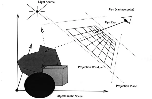
1-1 A sample scene illustrating a viewing location and direction, an eye
ray, a projection window and a light source . . . .
14
2-1 Pseudocode Braytrace's controlling function . . . .
18
2-2 Pseudocode for Braytrace's Trace function . . . .
19
2-3 Pseudocode for DRraytrace's controlling function . . . .
20
2-4 Pseudocode for DRraytrace's TraceProcRecurse function . . . .
21
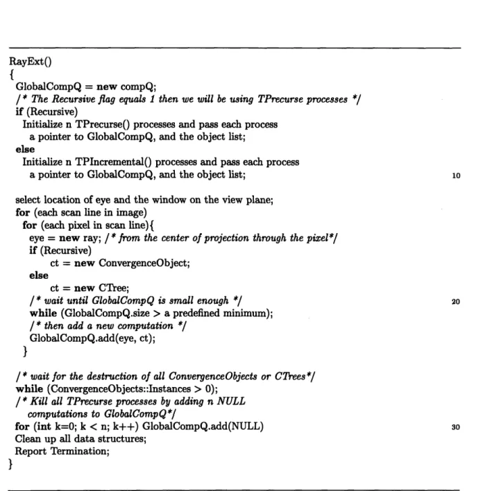
2-5 Pseudocode for DIraytrace's controlling function . . . .
23
2-6 Pseudocode for DIraytrace's TraceProcIncremental function . . . . .
24
3-1 Braytrace Flow Diagram ...
30
3-2 Object Inheritance and Data Dependency diagram for DRraytrace and
DIraytrace. Broken lines indicate a data dependency, solid lines
indi-cate a derived class ...
31
3-3 DRraytrace Flow Diagram ...
34
3-4 Simple Linked List Pseudocode . . . .
35
3-5 llmutex Pseudocode ...
. .
36
3-6 DIraytrace Flow Diagram ...
38
4-1
The Graphical User Interface of DTrace . . . .
42
7-1 The Graphic User Interface for the CTPlayer demonstration application. 54
7-2 The Graphic User Interface for the CTPlayer demonstration
applica-tion after skipping to an instrucapplica-tion . . . ..
56
7-3 The Graphic User Interface for the CTPlayer demonstration
applica-tion after advancing to a new locaapplica-tion in the CT file . . . .
.
57
7-4 The Graphic User Interface for the CTPlayer demonstration
List of Tables
4.1 Commandline options for DTrace
...
6.1 Runtime durations for the ray tracing algorithms . . . .
47
Chapter 1
Introduction
Ray tracing is an algorithm that creates a two dimensional image from a geometric
definition of a three dimensional scene. The two dimensional image is produced by
casting imaginary rays from a location in the scene (the viewer's eye), through a
window on an arbitrary viewing plane within the scene.
As a ray interacts with the objects in a scene, energy is conveyed back along that
ray to the pixel associated with the subdivision that defined that ray'. Once all the
calculations pertaining to the rays cast through a particular subdivision are complete,
the value of the pixel associated with that subdivision is set to the composite energy
of the rays cast through that subdivision (see Figure 1-1).
The images that a ray tracing algorithm is capable of producing are both realistic
and detailed. Shadows, reflection and refraction are just some of the effects that a ray
tracing algorithm can simulate. These effects are produced by performing extensive
calculations on the interactions between objects and rays.
As a ray intersects an object, that object's description and orientation are used to
create new rays which may pass through the intersected object (simulating refracted
light) or bounce off that object (simulating reflected light). These new rays, as
they intersect other objects in the scene, may themselves spawn new reflective and
refractive rays. A series of rays that is spawned from a single
root
ray is referred to
'The energy conveyed along a ray can also be thought of as the color of light that traverses that ray.
Light Source
Eye (vantage point)
Projection Plane n the Scene
Figure 1-1: A sample scene illustrating a viewing location and
a projection window and a light source.
direction, an eye ray,
as a ray tree. The final value of a pixel in the output image is then calculated by
converging the data contained in the one or more ray trees that are associated with
that pixel's corresponding subdivision.
The traditional implementation of a ray tracing algorithm uses a recursive calling
strategy to calculate and converge the data in a root ray's ray tree. The recursive
functions employed by such an implementation are controlled by a function that
iterates over each pixel in the output image. During each iteration of the controlling
function, one or more root rays are created and dispatched to the recursive ray tracing
function. This implementation of the ray tracing algorithm will be referred to as
Braytrace
2One fact of importance regarding the execution of Braytrace is that most of the
calculations performed to compute the energy along each ray are independent of all
other calculations. This computational independence leads to a concurrent
implemen-2
For a more detailed discussion on the basic ray tracing algorithm refer to [5].
I i
tation of the ray tracing algorithm which uses asynchronous symmetric processes to
calculate and converge the contribution of each individual ray that is created during
the rendering of a scene. This implementation of the ray tracing algorithm will be
referred to as DIraytrace.
The computational independence described above also leads to a second, simpler
concurrent implementation of the ray tracing algorithm. This second
implementa-tion uses the recursive strategy of Braytrace as the basis of its concurrent processes.
The concurrent processes used by this implementation work in parallel, each
recur-sively calculating the final value of a pixel in the output image. This concurrent
implementation of the ray tracing algorithm will be referred to as DRraytrace.
The remainder of this document describes the design and implementation of the
three ray tracing algorithms described above. The emphasis of this document will
be directed towards comparing and contrasting the DIraytrace algorithm with the
simpler, more straightforward DRraytrace algorithm, and the original Braytrace
al-gorithm.
The chapters in this document are organized as follows. Chapter 2 describes each
algorithm in more detail, giving pseudocode examples where necessary to illustrate
how the algorithms work. Chapter 3 gives a detailed description of the design and
im-plementation of the three algorithms. This chapter will include detailed descriptions
of all important functions and data objects. Chapter 4 describes DTrace, the user
interface to the ray tracing algorithms. Chapter 5 describes the debugging and testing
of the three algorithms. Chapter 6 describes the analysis conducted on the
concur-rent algorithms. The aim of this analysis is to compare and contrast the running time
and efficiency of the algorithms. Chapter 7 describes CTPlayer, an application whose
purpose is to demonstrate the expansion and convergence of ray trees as they created
and used by the DIraytrace algorithm. Then Chapter 8 discusses some conclusions
that can be drawn from the work described in this document.
Chapter 2
The Ray Tracing Algorithms
2.1
Braytrace
Braytrace stands for Basic Ray Tracing algorithm. Figure 2-1 shows the pseudocode
for RayExt, the controlling function of the Braytrace algorithm. As you can see
RayExt iterates over the entire projection window. During each iteration, RayExt
generates a ray defined by the pixel referenced in the current iteration. If the ray
fails to intersect an object in the scene, then the pixel is set to the background color.
If an intersection does occur, RayExt sets the current pixel to the value returned
by RayExt's call to the Trace function (see Figure 2-2). Once all the locations in
the output window have been iterated over and filled, the algorithm terminates and
returns the output buffer.
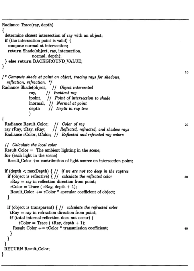
Trace is the entry point to the recursive ray tracing functions that are used by
RayExt to calculate the energy along each root ray. As can be seen in Figure 2-2,
Trace returns the value that is returned by its call to the Shade function. Shade
first calculates the local energy of the intersection point (due to direct lighting), then
adds to that the contributions due to reflected and refracted light. The reflected
and refracted contributions are calculated by returning the value that is returned by
Shade's recursive call to Trace.
/
* RayExt is the function that controls the execution of BRayExt
the recursive raytracing algorithm.*/
RayExt()
{
get the location of the eye and the size and location of the window on the view plane;
for (each scan line y) for (each pixel x)
{
create a ray that goes from the eye through pixel x,y;
OBJintersected = 0; o10
for (each object in the scene)
if (the object is intersected by the current ray) OBJintersected = 1;
//
set the value of the pixelif (OBJintersected) outMatrix[x,y] = Trace(ray, 1); else outMatrix[x,y] = BACKGROUND;
}// end for
Save or Return the outMatrix;
I
Figure 2-1: Pseudocode Braytrace's controlling function.
2.2
DRraytrace
DRraytrace is a straightforward parallelized extension of Braytrace. DRraytrace
stands for the Delegated Recursive Ray Tracer. It uses identical processes to
concur-rently calculate the values of individual pixels in the output image. These processes
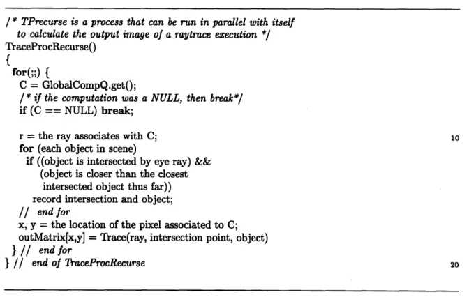
are named Recursive Trace (or TPrecurse) processes. Each TPrecurse process runs
an extended version of the recursive functions listed in Figure 2-2. The new function
is called TraceProcRecurse. The pseudocode for DRraytrace's controlling function
and TraceProcRecurse function can be found in Figure 2-3 and Figure 2-4.
As can be seen in Figure 2-3, RayExt once again iterates over the entire output
image, creating the root rays that will be used to calculate the pixel values. However,
since DRraytrace calculates the pixel values not by calling Trace, but by sending the
rays to the TPrecurse processes, a new form of communication between the calculation
functions and the controlling function is needed.
Communication between RayExt and TPrecurse processes is provided by an
in-stance of an object named compQ. A compQ object is a singly linked list, where the
Radiance Trace(ray, depth)
{
determine closest intersection of ray with an object; if (the intersection point is valid)
{
compute normal at intersection; return Shade(object, ray, intersection,
normal, depth);
} else return BACKGROUNDVALUE;
}
10
/
* Compute shade at point on object, tracing rays for shadows,reflection, refraction. */
Radiance Shade(object, // Object intersected
ray,
// Incident ray
ipoint, // Point of intersection to shade
inormal,
//
Normal at pointdepth // Depth in ray tree
)
{
Radiance ResultColor; // Color of ray 20
ray rRay, tRay, sRay; // Reflected, refracted, and shadow rays
Radiance rColor, tColor; // Reflected and refracted ray colors // Calculate the local color
Result-Color = The ambient lighting in the scene; for (each light in the scene)
ResultColor += contribution of light source on intersection point; if (depth < maxDepth)
{
// if we are not too deep in the raytreeif (object is reflective) {// calculate the reflected color 30
rRay = ray in reflection direction from point; rColor = Trace ( rRay, depth + 1);
Result-Color += rColor * specular coefficient of object;
}
if (object is transparent) {// calculate the refracted color tRay = ray in refraction direction from point;
if (total internal reflection does not occur)
{
tColor = Trace ( tRay, depth + 1);Result Color += tColor * transmission coefficient; 40
}
}
}
RETURN ResultColor;
Figure 2-2: Pseudocode for Braytrace's Trace function.
/
* RayExt controls the execution of the concurrent raytracing algorithms */RayExt()
{
GlobalCompQ = new compQ;
Initialize n TPrecurseo processes and pass each process a pointer to GlobalCompQ, and the object list; select location of eye and the window on the view plane; for (each scan line in image)
for (each pixel in scan line){ 10
eye = new ray; /* from the center of projection through the pixel*/
ct = new ConvergenceObject; /* for the current pixel*/
/ * wait until GlobalCompQ is small enough */
while (GlobalCompQ.size > a predefined minimum);
/
* then add a new computation */GlobalCompQ.add(eye, ct);
}
/*
wait for the destruction of all ConvergenceObjects */while (ConvergenceObjects::Instances > 0); 20
/* Kill all TPrecurse processes by adding n NULL
computations to GlobalCompQ*/
for (int k=0; k < n; k++) GlobalCompQ.add(NULL) Clean up all data structures;
Report Termination;
}
/*
TPrecurse is a process that can be run in parallel with itself to calculate the output image of a raytrace execution */TraceProcRecurse() 30
{
for(;;) {
C = GlobalCompQ.get(;
/
* if the computation was a NULL, then break*/if (C == NULL) break;
r = the ray associates with C; for (each object in scene)
if ((object is intersected by eye ray) &&
(object is closer than the closest 40
intersected object thus far)) record intersection and object;
// end for
x, y = the location of the pixel associated to C; outMatrix[x,y] = Trace(ray, intersection point, object)
}// end for
}
/*
TPrecurse is a process that can be run in parallel with itself
to calculate the output image of a raytrace execution */
TraceProcRecurse()
{
for(;;) {
C = GlobalCompQ.getO;
/ * if the computation was a NULL, then break*/
if (C == NULL) break;
r = the ray associates with C; 10
for (each object in scene)
if ((object is intersected by eye ray) && (object is closer than the closest
intersected object thus far)) record intersection and object;
// end for
x, y = the location of the pixel associated to C; outMatrix[x,y] = Trace(ray, intersection point, object)
}// end for
}
//
end of TraceProcRecurse
20Figure 2-4: Pseudocode for DRraytrace's TraceProcRecurse function.
data at each location of the list is what will be referred to as a Ray Intersect
Com-putation (RIC). An RIC is an object that contains a pointer to a ray, and a pointer
to a location where the result of the ray trace calculations can be stored.
A single instance of the compQ data object is shared by all concurrent processes,
this instance is called GlobalCompQ. Once a TPrecurse process extracts an RIC from
GlobalCompQ, it uses the ray within the RIC as an argument to the Trace function.
The value returned by Trace is then placed into the output buffer location defined in
the RIC.
2.3
Dlraytrace
As was stated in the introduction, all rays can be calculated independently of one
an-other. Dlraytrace seeks to exploit the independence of computation associated each
individual ray. The concurrent processes that DIraytrace controls are called
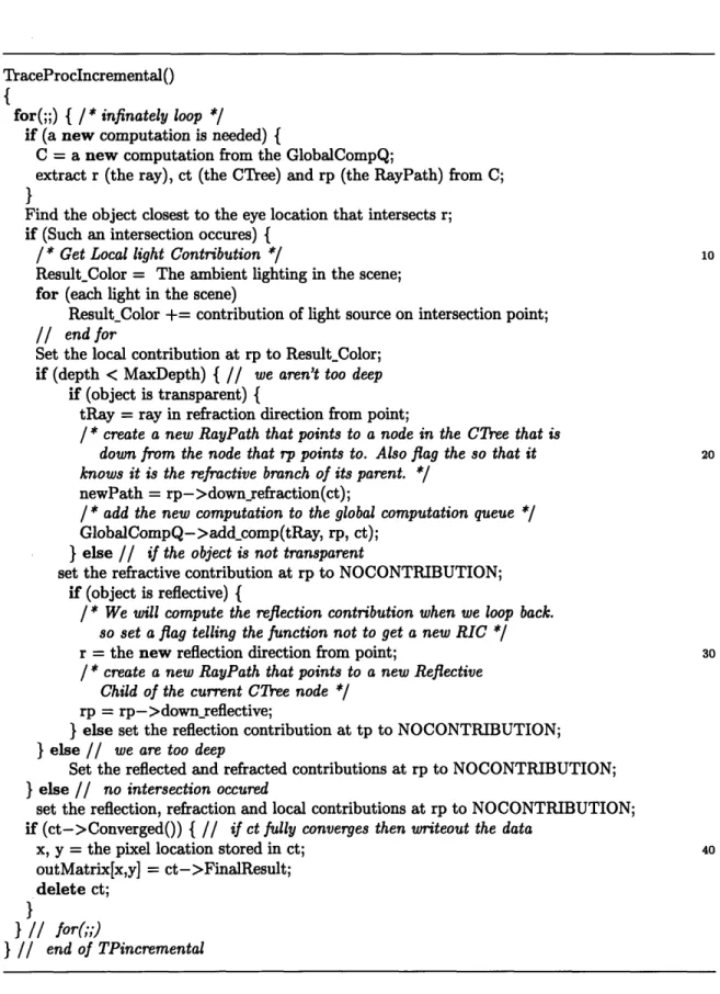
Incre-mental Trace (or TPincreIncre-mental) processes. The main function of a TPincreIncre-mental
process is called TraceProcIncremental.
As can be seen in the pseudocode listed in Figure 2-5, DIraytrace introduces two
new data objects, the Convergence Tree (CTree) and the Ray Path. Instances of both
of these objects are sent with each ray that RayExt places in the GlobalCompQ. When
a TPincremental process finishes a calculation, it uses the Ray Path to reference the
location in the CTree where the calculated data should be placed.
CTrees are shared data objects, this allows TPincremental processes to
concur-rently place data into different locations in a particular CTree. This is important due
to the fact that a number of processes may be concurrently calculating values for a
single CTree.
When enough information has been placed in a CTree, a TPincremental process
will converge the data in the CTree. The converged result is then used as a
contribu-tion to the final value of the pixel associated with the CTree.
2.4
Extra Features
A number of visual effects can be produced by making simple modifications to the
basic and concurrent ray tracing algorithms. Two such modifications,
Supersam-pling and Spectral Distribution calculations, are realized in the implementations of
Braytrace, DRraytrace and DIraytrace.
2.4.1
Supersampling
Supersampling refers to the casting of multiple rays through a single subsection in the
projection window. The thing to keep in mind is that each subsection in the projection
window possesses an area. Supersampling is performed by projecting multiple, slightly
offset rays through each location in the window, and then averaging the results of the
calculations associated with each ray.
The visual result of supersampling is that edges are "softer" or less distinct, and
details that may have not contributed to the output image due to the sparseness of
the subsections in the projection window, will now have some effect on the output
RayExt()
{
GlobalCompQ = new compQ;
/
* The Recursive flag equals 1 then we will be using TPrecurse processes */if (Recursive)
Initialize n TPrecurseo processes and pass each process a pointer to GlobalCompQ, and the object list; else
Initialize n TPIncremental() processes and pass each process
a pointer to GlobalCompQ, and the object list; o10
select location of eye and the window on the view plane; for (each scan line in image)
for (each pixel in scan line){
eye = new ray; /* from the center of projection through the pizel*/
if (Recursive)
ct = new ConvergenceObject; else
ct = new CTree;
/* wait until GlobalCompQ is small enough */ 20so while (GlobalCompQ.size > a predefined minimum);
/
* then add a new computation */GlobalCompQ.add(eye, ct);
}
/ * wait for the destruction of all ConvergenceObjects or CTrees*/
while (ConvergenceObjects::Instances > 0);
/* Kill all TPrecurse processes by adding n NULL
computations to GlobalCompQ*/
for (int k=0; k < n; k++) GlobalCompQ.add(NULL) 30
Clean up all data structures; Report Termination;
}
TraceProcIncremental()
{
for(;;)
{ /
* infinately loop */
if (a new computation is needed) {
C = a new computation from the GlobalCompQ;
extract r (the ray), ct (the CTree) and rp (the RayPath) from C;
}
Find the object closest to the eye location that intersects r; if (Such an intersection occures) {
/ * Get Local light Contribution */ O10
Result-Color = The ambient lighting in the scene; for (each light in the scene)
Result_Color += contribution of light source on intersection point;
// end for
Set the local contribution at rp to Result_Color; if (depth < MaxDepth)
{
// we aren't too deepif (object is transparent) {
tRay = ray in refraction direction from point;
/*
create a new RayPath that points to a node in the CTree that isdown from the node that rp points to. Also flag the so that it 20
knows it is the refractive branch of its parent. */
newPath = rp->downrefraction(ct);
/
* add the new computation to the global computation queue */GlobalCompQ->addcomp(tRay, rp, ct);
} else
//
if the object is not transparentset the refractive contribution at rp to NOCONTRIBUTION; if (object is reflective) {
/*
We will compute the reflection contribution when we loop back. so set a flag telling the function not to get a new RIC */r = the new reflection direction from point; 30
/*
create a new RayPath that points to a new Reflective Child of the current CTree node */rp = rp->downreflective;
} else set the reflection contribution at tp to NOCONTRIBUTION; } else
//
we are too deepSet the reflected and refracted contributions at rp to NOCONTRIBUTION;
} else
//
no intersection occuredset the reflection, refraction and local contributions at rp to NOCONTRIBUTION; if (ct->Converged0)
{
//
if ct fully converges then writeout the datax, y = the pixel location stored in ct; 40
outMatrix[x,y] = ct->FinalResult; delete ct;
}
} i/ for(;;)
}
//
end of TPincrementalimage.
To perform the supersampling of an output image, Braytrace must create the
supersample rays, then average their return values.
To accomplish supersampling in the DRraytrace algorithm, RayExt must creates
the supersample rays, and then send a single instance of a new data object, the
supersample Convergence object (supConvObj), to the TPrecursive processes. This
new object possesses functionality which facilitates the convergence of supersampled
data.
DIraytrace works in a way similar to that of DRraytrace. However, instead of
using the supConvObj object, DIraytrace uses an object derived from CTree. This
new object is called a Supersample Convergence Tree object (supCTree).
2.4.2
Spectral Distribution Calculations
Spectral Distribution (SPD) calculations take into account the fact that materials
possess different refractive properties for different wavelengths of light. One example
of this phenomenon is the way in which a crystal refracts white light. Since a crystal
has a different refractive index for different wavelengths of light, the light that exits
a crystal is a spectrum that is spread over an area (as opposed to a simple beam of
white light).
To perform SPD calculations, each object in the scene is given three refractive
indices corresponding to red, green or blue light. Then, when a ray hits an object,
three refraction rays (one for each index) are cast rather than one. When converging
the ray tree to which the refractive rays belong, only the color of light for which a
ray was cast will contribute to the final result. For example if a white light strikes a
crystal, three refractive rays (a red ray, a green ray and a blue ray) are cast. Then,
when converging the ray tree, only the red contribution of the red transmission ray,
the green contribution of the green ray and the blue contribution of the blue ray will
be used in final result of the ray tree.
To implement SPD calculations, the way in which recursive rays are created must
be modified. Braytrace and DRraytrace must now spawn three transmission rays,
then scale the values that are returned for each ray. The scaled results can then be
used as contributions to the ray tree's final value.
The modifications to DIraytrace are very similar to the modification made to
Braytrace and DRraytrace. DIraytrace must create three refractive rays instead of
one, then converge the resulting contributions of the three rays. The difference
be-tween DIraytrace and the other two algorithms is that instead of making a recursive
function call to calculate the energy of each recursive ray, DIraytrace places a new ray
into the GlobalCompQ so that an idle process can calculate that ray's contribution.
Chapter 3
Implementations of the Ray
Tracing Algorithms
The pseudocode in the previous chapter hides many important implementational
is-sues. For example what primitives are used in the Braytrace algorithm? What
mech-anisms are employed by DRraytrace and DIraytrace to synchronize the concurrent
processes? How does DIraytrace converge a CTree?
This chapter will describe the functions and data objects that are used to realize
the algorithms detailed in the previous chapter.
3.1
Braytrace
Let us first discuss the implementation of the Braytrace algorithm'. Let us begin
by describing the data structures and functions used by Braytrace. Then we shall
describe the calling sequence of the functions that control the algorithm.
3.1.1
Braytrace: Data Objects and Functions
Many of the data objects used in Braytrace are provided by or derived directly from
objects that are defined in the Silicon Graphics InventorGL graphics library [4].
1
The code and data objects for the Braytrace algorithm are taken from code used in a Computer
Below is a list describing the data objects and functions used by Braytrace
2Point: Point encapsulates the three coordinates that define a location in a scene.
ObjectData: ObjectData describes an object in a scene. It encapsulates such
in-formation as the type of material that the object is made of (used for the
calculation of transmitted and reflected rays), the location and orientation of
the object, and the faces, vertices and edges that define the object.
LightData: LightData describes a light source in the scene. It encapsulates such
information as the light's location, direction, color and intensity.
Octree: Octree is a data object that is used to store and retrieve all the entities in
a scene. It possesses member functions that allow a caller to add objects to a
scene, search for objects in a scene and list all the objects in a scene.
Ray: Ray encapsulates information used to describe rays that are cast by the ray
tracing algorithms. The information that Ray encapsulates includes a ray's
ori-gin and direction, a Spectral Distribution mask (used for Spectral Distribution
Calculations), and an ObjectData pointer that points to an object that the ray
may be propagating through (used for transmission calculations).
Hit: Hit describes an intersection that has occurred between a ray and an object.
It contains a pointer to the object, the location of the intersection, the normal
vector at the point of the intersection, and whether the ray was entering of
leaving the object.
ViewVolume: ViewVolume contains information on how the scene will be viewed.
The information it encapsulates includes the location and orientation of the
viewer of the scene, the distance from the location of the viewer to the projection
plane and the distance from the viewer to the farthest objects that will appear
in the output image (these distances are often referred to as the near and far
clipping planes).
Radiance: Radiance is used to encapsulate data that describes a color. The
in-formation contained in a Radiance object is composed of three floating point
values ranging from 0 to 1. Each value corresponds to the amount of red, green
or blue light in the composite color.
setPixel(...): The setPixel function is used to set the value of a pixel in the output
image. Its arguments are an <x,y> coordinate and a Radiance. A pointer to
a setPixel function is passed to a ray tracing algorithm during that algorithm's
initialization. Then, as the algorithm executes, the setPixel function is used to
store the pixel values that are calculated by the algorithm.
2In this list and all lists to follow, "<objl> -> <obj2>" means that obj2 inherits all data and functionality encapsulated in objl.
RayExt(...): RayExt is the controlling function of all three ray tracing algorithms.
Its arguments include an array of ObjectData (containing the objects in the
scene), an array of LightData (containing the lights in the scene), a pointer to
a ViewVolume and a pointer to a setPixel function.
ivTrace(...): The ivTrace function is an implementation of the Trace function
de-scribed in Section 2.1. It takes as its arguments a Ray, an Octree containing
the objects in a scene, a depth, a weight and an index of refraction. It returns
the Radiance along the given Ray. The depth and weight are used for recursion
termination.
ivIntersect(...): The ivIntersect function takes as its arguments a Ray, an Octree
containing the objects in a scene, and a pointer to a Hit object. Its return type
is an integer. If the ray intersects an object in the scene, then the Hit object
pointed to by the Hit pointer is modified to describe the intersection, and a 1
is returned to the caller. Otherwise 0 is returned.
ivShade(...): The ivShade function takes as its arguments a pointer to a Hit object,
a viewing direction, a Spectral Distribution mask, an Octree containing a list of
objects in the scene, an array of LightData containing the lights in the scene and
the depth and weight values from ivTrace. The ivShade function then returns
a Radiance object that contains the color at the intersection contained in the
Hit object.
The code for these objects and functions can be found in Appendix D.
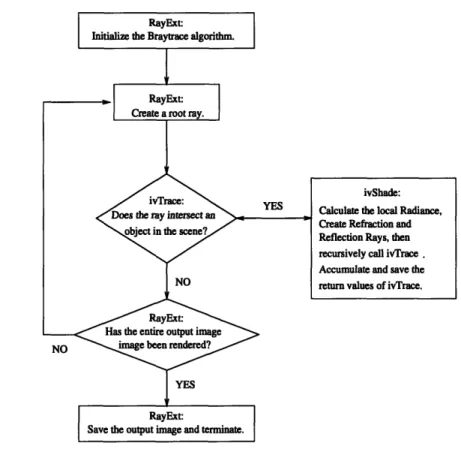
3.1.2
Braytrace: Calling Sequence
Figure 3-1 contains a flow diagram describing the calling sequence of the Braytrace
algorithm. The figure illustrates the recursive function calling that is employed by
the Braytrace algorithm.
3.2
DRraytrace and DIraytrace
A number of new data objects and functions are needed to realize the DRraytrace
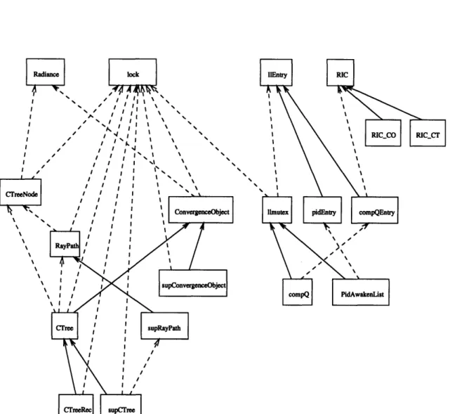
and DIraytrace algorithms. Figure 3-2 contains an inheritance diagram that shows
the objects that are used by the concurrent algorithms.
As you can see, most of the new objects use the shared data object lock. The
lock object is what is referred to as a Mutual Exclusion (mutex) object. Mutex
Figure 3-1: Braytrace Flow Diagram
objects are one of the most basic synchronization
3mechanisms used by concurrent
algorithms. The validity and efficiency of a mutex object is central to the performance
and correctness of concurrent algorithms. For a more thorough discussion on mutual
exclusion objects refer to [7].
3.2.1
DRraytrace: Objects and Functions
Below is a list containing all the new data objects and functions used by the
DRray-trace algorithm.
ConvergenceObject: ConvergenceObject is a base object (i.e. other objects will
be derived from it) that encapsulates functionality and information needed to
converge ray tracing calculations to an output Radiance. ConvergenceObject
possesses a pointer to a setPixel function. It also contains data describing the
number of ConvergenceObject instances in existence (the number of existing
instances is used to check for termination of the algorithm).
3
Synchronization refers to the action of getting asynchronous, concurrently executing processes
' %
Radiance
A I -CTreeNode 1 1Figure 3-2: Object Inheritance and Data Dependency diagram for DRraytrace and
DIraytrace. Broken lines indicate a data dependency, solid lines indicate a derived
class.
supConvergenceObject: (ConvergenceObject->supConvergenceObject)
supConver-genceObject is a ConversupConver-genceObject that possess the additional functionality
and data needed to converge ray tracing calculations that are performed during
the creation of a supersampled output image.
RIG: RIG stands for Ray Interception Computation. It describes a concurrent ray
tracing computation. RIC is a base class from which specialized RICs are
defined. The only data that is encapsulated by a base RIC object is a Ray.
RICCO: (RIC->RICCO) RICGCO is an RIC that additionally possesses a pointer
to a ConvergenceObject (this pointer may also point to a
supConvergenceOb-ject). RICGCO objects are used to convey root rays to TPrecurse processes.
lock: A lock is a mutual exclusion object. These objects are shared by concurrent
processes. They are used in situations where concurrent processes may interfere
with one another, or where the synchronization of concurrently executing
pro-cesses is needed. A lock can be "acquired" or "released". Once a lock is acquired
it cannot be acquired again until it is released. The lock object is implemented
using an abilock.t data structure. These data structures are primitive mutual
exclusion objects that are built into Silicon Graphics' Iris Unix operating system
[1].
llmutex: The llmutex object is a sharable singly linked list. It can be accessed
si-multaneously by multiple concurrently executing processes. It uses lock objects
to ensure the integrity of the list even when the list is being accessed
simul-taneously by multiple processes. The llmutex object is a base class for more
specialized sharable linked lists.
llEntry: The llEntry object is a node in an llmutex list.
compQEntry: (llEntry->compQEntry) The compQEntry object is an llEntry that
contains a pointer to an RIC object (note that a pointer to an RIC object can
also point to any object derived from an RIC object).
compQ: (llmutex->compQ) The compQ object is a linked list of compQEntries.
This new linked list provides functions for adding and retrieving RIC objects.
It further provides functions for waiting on the availability of RIGs in the list.
These wait functions are used so that a process that is waiting for an RIC, can
be informed when an RIC is available.
pidEntry: (pidEntry->llEntry) A pidEntry is an llEntry that contains a process
identifier, and a lock.
PidAwakenList (llmutex->PidAwakenList) A PidAwakenList is an llmutex object
that allows a calling process to add itself to a list of processes that are waiting
to be awakened by some other process. It also allows a process to awaken some
or all of the processes that are in the list. PidAwakenList uses pidEntry nodes
to keep track of what processes are in the list. The mechanism for awakening
processes in a PidAwakenList uses the lock that is contained in the pidEntry
object. When a process wishes to be added to a PidAwakenList, it calls a
member function of the list which returns a lock object that has already been
acquired. The process then attempts to reacquire the lock. Since the lock is
already acquired, the process must wait until the lock is release before it can
continue executing its code. The list, when informed that it should awaken
a process, will release the lock that is associated with that process, thereby
enabling the process to acquire its lock and proceed with its computations. The
compQ object uses the PidAwakenList as a means of telling processes that RICs
are available.
TraceArg: TraceArg encapsulates information that is needed when initializing
TPre-cursive processes. The TraceArg data object contains pointers to a compQ
ob-ject, an Octree data object and a LightData array which contains the lights in
the scene.
sproc(...): The sproc function [2] is a function call that "forks" off new processes.
It is used to initialize the TPrecursive and TPincremental processes. One of its
arguments is a pointer that will be passed to the forked process. This pointer
is used to transmit a TraceArg object from RayExt to the TPrecursive and
TPincremental processes.
RayExt(...): RayExt is the function that supervises the execution of all the ray
tracing algorithms. When RayExt is controlling the DRraytrace algorithm,
it creates a single GlobalCompQ object. Then it uses sproc to initialize the
TPrecursive processes. RayExt then iterates over the pixels in the output image,
creating root rays and RICs that will be sent to the current processes via the
GlobalCompQ. Lastly, when all pixels have been iterated over, RayExt reports
the termination of the algorithm.
TraceProcRecurse(...): TraceProcRecurse is the main function of a TPrecursive
process. Upon initialization it gets the TraceArg object that was sent to it by
RayExt, and from that object it extracts all the information that it needs to
ini-tialize itself. Then it waits for an RIC to become available in the GlobalCompQ.
Once an RIC is available it calculates the radiance along the ray contained in
the RIC, then records the result in the output image location specified in the
RIC. Once a computation is complete, TraceProcRecurse loops back and waits
for the next RIC to become available. TraceProcRecurse interprets a NULL
RIC as a signal that RayExt wants the process to terminate.
These objects and functions possess the functionality that is needed to perform
the DRraytrace algorithm. The source code for these objects and functions can be
found in Appendix E.
Figure 3-3: DRraytrace Flow Diagram
3.2.2
DRraytrace: Calling Sequence
Figure 3-3 contains a flow diagram describing the calling sequence for the DRraytrace
algorithm. This figure illustrates the division of labor that exists in the DRraytrace
algorithm. This division is facilitated by the communication that takes place via the
GlobalCompQ.
One important quality that the GlobalCompQ must possess is that it must
guar-antee that only one process can retrieve any particular RIC. Let us look at an example
of why such a guarantee is needed.
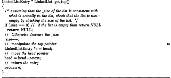
Figure 3-4 contains the pseudocode for a function that extracts the first element
from a standard singly linked list. In the case where only one process will execute this
function, the code in the figure is valid. However it is not difficult to derive examples
where if two processes are executing this code nearly simultaneously, the code yields
LinkedListEntry * LinkedList::gettop()
{
/*
Assuming that
the _size of the list is consistent with
what
is actually in the list, check that the list is
non-empty by checking the size of the list.
*/
if (_size
==
0)// if the list is empty than return NULL
return NULL;
//
Otherwise decrease the _size
size--;
// manipulate the top pointer
io
LinkedListEntry *e
=
head;
//
move the head pointer
head
=
head->next;
// return the entry
return e;
}
Figure 3-4: Simple Linked List Pseudocode
incorrect results.
Example:
1. Process i enters the get-top function and checks the _size variable. The size
variable is currently set to 1.
2. Process
j
enters the get-top function and checks the _size variable. The -size
variable is still 1.
3. Processes i and
j
then both attempt to get the element in the list. Since they
both decrease the -size variable, the _size is now set to -1.
4. Both i and
j
then set their respective e pointers to head.
5. i then sets head = head->next. The result of this instruction is that head is
now set to NULL.
6.
j
tries to set head
=
head->next, but since head is already set to NULL this
instruction causes an invalid pointer reference.
This example shows the incorrectness of this function when it is being concurrently
executed by multiple processes.
Now look at the pseudocode for llmutex's get-top member function (refer to
Fig-ure 3-5). This code prevents errors like the ones in the example just given by limiting
the critical retrieval code to one process at a time. Such exclusion policies are present
llEntry *llmutex::get_top()
{
// check if the list is nonempty
if (_size == 0) return NULL;
// lock the _size
sizeLock.lockresource(TRUE);
//
recheck _size
if (_size == 0) {
sizeLock.unlockresourceO;
return NULL; 10}
//
manipulate _size
size--;
// lock, manipulate and unlock top
headLock.lockresource();
llEntry *e
=
head;
head
=
head->next;
headLock.unlockresource();
sizeLock.unlock_resource();
//
return the element
20return e;
}
Figure 3-5: llmutex Pseudocode
in most of the shared object classes used in the DRraytrace and DIraytrace
algo-rithms.
3.2.3
DIraytrace: Objects and Functions
Below is a list containing the new data objects and functions that are used by
DIray-trace.
CTree: (ConvergenceObject->CTree) CTree is an object that represents a ray tree.
It provides functions to traverse the tree, and set values within the tree.
CTreeNode: CTreeNode is a node in a CTree. It contains node pointers that point
to a node's reflective child, refractive children, and parent. It also contains
Spectral Distribution, weight and scaling coefficient information. Lastly it
con-tains a lock object and a integer flag. These last two data objects are used to
ensure the correct convergence of the data in the CTree.
CTreeRec: (CTree->CTreeRec) CTreeRec is a CTree that has the added capability
of saving a log of the creation and convergence of the CTree to an external
data file. This log is created by augmenting all the functions that manipulate
the CTree object with commands that write to a log file (see Chapter 7 and
Appendix B for more information on CTreeRec and log files).
RayPath: RayPath is a data object that specifies a location in a CTree or CTreeRec
object. It contains a pointer to a node in a CTree as well as functions that allow
a caller to traverse and create new nodes in a CTree.
RICCT: (RIC->RIC.CT) RICCT is an RIC object that includes a pointer to a
CTree object and a pointer to a RayPath object. RIC.CT objects are created by
RayExt when RayExt is controlling TPincremental processes. RIC-CT objects
are also created by TPincremental processes when they need to delegate work
to other TPincremental process.
supCTree: (CTree->supCTree) The supCTree object is a CTree that possesses
ad-ditional data and functionality to support the supersampling of a scene. It does
this by storing an array of CTrees, and then converging the final result of each
CTree to a composite radiance for the entire supCTree object.
supRayPath: (RayPath->supRayPath) The supRayPath object is a RayPath that
is used when referencing supCTree objects. In addition to the data that is
con-tained in a standard RayPath object, supRayPath also indicates which CTree
within a supCTree object is being referred to.
RayExt(...): RayExt, when controlling the DIraytrace algorithm, creates CTree,
CTreeRec or supCTree objects for the RICs that are sent to the
TPincremen-tal processes (supCTree objects are created if supersampling is enabled, and
CTreeRec objects are created when a log of the creation and convergence of the
CTree is needed).
TraceProcIncremental(...): TraceProcIncremental is the main function of a
TPin-cremental process. Its execution is best described as a merging of the
Trace-ProcRecursive and ivShade functions. TraceProcIncremental extracts the next
available RICGCT object from GlobalCompQ. It then checks if the ray in the
RIC intersects an object in the scene. If an intersection occurs, then the local
radiance at the intersection point is calculated (by calling ivShade) and stored
in the CTree. If needed, reflective and refractive rays, as well as RICCT objects
to store those rays, are created and added to GlobalCompQ.
TraceProcIncre-mental then loops back and if the last computation spawned a reflection ray, it
calculates the radiance of that ray and places the result into the CTree. When
TraceProcIncremental can no longer calculate or converge data for the current
RICGCT, it discards that RIC and attempts to acquire a new RICGCT object
from the GlobalCompQ. Just as with TraceProcRecursive,
TraceProcIncremen-tal interprets the retrieval of a NULL RICCT from the GlobalCompQ as an
indication that RayExt wants the process to terminate.
Figure 3-6: DIraytrace Flow Diagram
These objects and functions possess the functionality that is needed to execute
the DIraytrace algorithm. The source code for these objects and functions can be
found in Appendix E.
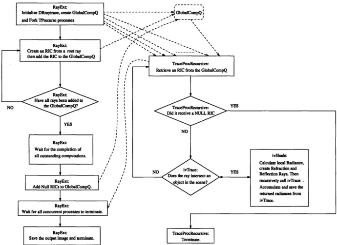
3.2.4
DIraytrace: Calling Sequence
Figure 3-6 contains a flow diagram that describes the calling sequence of the
DI-raytrace algorithm. As you can see, the execution of the RayExt function remains
primarily unchanged. The major difference between the execution of this algorithm
and the execution of the DRraytrace algorithm is the non recursive nature of the
TPincremental process.
3.2.5
DIraytrace: Convergence of CTree Data
One important aspect of the DIraytrace implementation that is hidden by the CTree
object class is the issue of which process actually converges the data in a CTree.
The answer to this question lies in the implementation of the CTree object. In
particular the SetReflected, SetRefracted and SetLocal member functions of CTree
and its derived types.
CTree::SetReflected, CTree::SetRefracted and CTree::SetLocal take as arguments
a Radiance, and a RayPath
4. Once the radiance is recorded in the node, a private
member function named Converge is called
5.
Converge attempts to converge the data in the CTree. Converge's only argument is
a RayPath. Converge extracts from that RayPath object the CTreeNode from which
convergence should be attempted. The mutex lock that is contained within each
CTreeNode is used to figure out what process converges the data that is contained in
the node.
When a process calls one of the set functions, the lock for that node will be
acquired, thus preventing other processes from setting a value in that node, or
con-verging the data in that node. Once a process has the lock for a node, it will, after
setting the data in the node, attempt to converge the data in that node to the node's
parent. If successful the node's flag is set to a value that indicates that the node has
been converged. Once a process has attempted to converge the data in a node, it will
release the node's lock and exit the Set function.
Once a CTree is filled, one of the last processes (but not necessarily the last
process) that attempts to converge the tree will succeed.
4The SetRefracted function also takes an integer that indicates which Spectral Distribution
con-tribution needs to be set.
Chapter 4
User Interface
4.1
Graphic User Interface
All three of the rendering algorithms just described are incorporated into a single
program named DTrace. DTrace's user interface is mostly based on an interface that
was provided with the code from Seth Teller's class. This interface was created using
the OpenGl application development toolkit [3].
To provide access to the DRraytrace and DIraytrace algorithms, various additions
have been made to the original interface.
Figure 4-1 shows the graphic user interface of DTrace. Small modifications have
been made to the button list on the left side of the window. The three buttons that
appear on the left side are now linked to the three different rendering algorithms
(Braytrace, DRraytrace and DIraytrace). Other than this change, the interface is the
same as it was originally.
Some of the other controls that are available through the graphic interface provide
ways of manipulating the lighting in the scene, and changing the orientation of the
eye of the viewer.
Figure 4-1: The Graphical User Interface of DTrace.
4.2
Commandline Interface
The original code also implemented a very limited command line interface. This
interface simply set certain flags which defined how Braytrace would execute. To
help with the testing and debugging of the concurrent algorithms, the command line
interface was expanded.
As you can see in Table 4.1 the commandline parameters are divided into old and
new options. The old options mostly pertain to the common elements of all three
algorithms, while the new options are mostly needed for the concurrent algorithms.
Some of the most important new options allow a user to not only set the
pa-rameters used by the concurrent algorithms, but to indicate that the image should
be rendered immediately using the information on the command line. The options
that provide for the immediate rendering of an image are -eye <eye file> and -UI
<interface mode>.
Ap-OLD OPTIONS:
[-script <file name> [-c]] [-read <file name> [-i N] [-c]] [-m rendermode]
Inventor Raytrace [-f <base file name>] [-o] [-d maxraydepth >= 0] [-e environ.iv] [-j (itter samples)] [-p N (cast N x N rays/pixel) >= 1] [-eye <filename> [-s shademode ( Flat Normal Ambient Local Direct Recursive)]
E-v
minrayweight >=0] C-D debuglevel >=0] [-d (- for stdin)] NEW OPTIONS:[-dell
(delegate computations)[-n nprocesses] (nprocess >= 1; default = 2) [-UI <line I gl>]
[-size v h] (in glmode just resize the window, otherwise default = 50x50)
[file.iv (- for stdin)]
[-CT <file name>]
[-old]
(use the old raytracer tracer)[-help]