On sunspot fluctuations in variable capacity utilization models

HAL Id: hal-01729346

https://hal-amu.archives-ouvertes.fr/hal-01729346

Submitted on 1 Apr 2019

HAL is a multi-disciplinary open access

archive for the deposit and dissemination of

sci-entific research documents, whether they are

pub-lished or not. The documents may come from

teaching and research institutions in France or

abroad, or from public or private research centers.

L’archive ouverte pluridisciplinaire HAL, est

destinée au dépôt et à la diffusion de documents

scientifiques de niveau recherche, publiés ou non,

émanant des établissements d’enseignement et de

recherche français ou étrangers, des laboratoires

publics ou privés.

On sunspot fluctuations in variable capacity utilization

models

Frederic Dufourt, Alain Venditti, Rémi Vivès

To cite this version:

Frederic Dufourt, Alain Venditti, Rémi Vivès.

On sunspot fluctuations in variable

capac-ity utilization models.

Journal of Mathematical Economics, Elsevier, 2018, 76 (C), pp.80-94.

On sunspot fluctuations in variable capacity utilization models

✩

Frédéric Dufourt

a

, Alain Venditti

a,b,

*

, Rémi Vivès

a

a_{Aix-Marseille University, CNRS, EHESS, Centrale Marseille, AMSE, Marseille, France} b_{EDHEC Business School, France}

a b s t r a c t

We investigate the extent to which standard one sector RBC models with positive externalities and variable capacity utilization can account for the large hump-shaped response of output when the model is submitted to a pure sunspot shock. We refine the Benhabib and Wen (2004) model considering a general type of additive separable preferences and a general production function. We provide a detailed theoretical analysis of local stabilities and local bifurcations as a function of various structural parameters. We show that, when labor is infinitely elastic, local indeterminacy occurs through Flip and Hopf bifurcations for a large set of values for the elasticity of intertemporal substitution in consumption, the degree of increasing returns to scale and the elasticity of capital–labor substitution. Finally, we provide a detailed quantitative assessment of the model and conclude with mixed results. We show that although the model is able theoretically to generate a hump-shaped dynamics of output following an i.i.d. sunspot shock under realistic parameter values, the hump is too persistent for the model to be considered fully satisfactory from an empirical point of view.

1. Introduction

In this paper, we emphasize the link between demand shocks and expectation-driven fluctuations based on the existence of sunspot equilibria. More precisely, we investigate the extent to which standard one-sector sunspot models with positive external-ities and variable capacity utilization can account for ‘‘boom-bust cycles’’ characterized by procyclical covariations of most macroe-conomic variables and a hump-shaped output response when the model is submitted to a pure sunspot shock.

✩_{This work has benefited from the financial support of the French National}

Research Agency (ANR-15-CE33-0001-01). We thank the co-editor A. Citanna and an anonymous referee together with N. Abad, S. Bosi, R. Boucekkine, L. Kaas, F. Magris, C. Nourry, C. Poilly and T. Seegmuller for useful comments and suggestions. This paper also benefited from presentations at the ‘‘Doctoral Workshop on Quan-titative Dynamic Economics’’, GREQAM, Marseille, September 2016, the Interna-tional Workshop on ‘‘Financial and real interdependencies: volatility, internaInterna-tional openness and economic policies’’, GREQAM, Marseille, November 2016, the 21st Conference ‘‘Theories and Methods in Macroeconomics’’, Católica Lisbon School of Business & Economics, Lisbon, March 2017, the Seminar in Macroeconomics, University of Konstanz, April 2017, the ASSET Metting, Algiers, October 2017, the 6th Annual Lithuanian Conference on Economic Research, Vilnius, June 2017, and the International Conference on ‘‘Real and Financial Interdependencies : New Approaches with Dynamic General Equilibrium Models’’, Paris School of Economic, Paris, July 2017.

*

Corresponding author at: Aix-Marseille University, CNRS, EHESS, Centrale Mar-seille, AMSE, MarMar-seille, France and EDHEC Business School, France.

E-mail addresses:frederic.dufourt@univ-amu.fr(F. Dufourt),

alain.venditti@univ-amu.fr(A. Venditti),remi.vives@univ-amu.fr(R. Vivès).

The traditional view put forward in the DSGE literature is that fluctuations are triggered by shocks on economic fundamentals. However, sinceCass and Shell(1983), a field of economic research has been developed to analyze the role of agents’ expectations in the understanding of macroeconomic fluctuations. In particular, researchers have highlighted the fact that agents can collectively change their expectations due to exogenous reasons, not necessar-ily related to economic fundamentals. In turn, these changes in ex-pectations generate fluctuations which validate ex-post the initial expectations and are thus consistent with rational expectations, i.e. sunspot fluctuations are based on self-fulfilling prophecies.

The first sunspot model using the framework of the RBC/DSGE literature (Benhabib and Farmer, 1994) was shown to perform as well as, or even better than, the canonical RBC model (Farmer and Guo, 1994). However, a major hurdle this literature faced was that the existence of sunspot equilibria required very large levels of increasing returns to scale, inconsistently with the data. This weak-ness was considered one of the main challenge for the macroe-conomic sunspot literature untilWen(1998) proposed a simple extension consisting in introducing a variable capital utilization rate in the Benhabib–Farmer setup, in the spirit ofGreenwood et al.(1988).1 It was shown that this simple extension to the canon-ical one-sector model was sufficient to allow for the existence of sunspot fluctuations under low and empirically plausible levels of

1_{An alternative explanation is to introduce a two-sector setup with increasing}

increasing returns. Moreover,Benhabib and Wen(2004) showed that this model could also explain many dimensions of observed business cycles when the model is submitted to correlated fun-damental and sunspot shocks. In particular, the model is able to account for Pigou cycles: periods of booms and busts triggered by exogenous changes in agents’ expectations and affecting most macroeconomic variables. The Benhabib–Wen (henceafter BW) model then put an end to years of discussions about the credibility of sunspot models and their ability to explain salient features of observed business cycles.

Yet, a careful examination of the results presented by BW re-veals that there remains one dimension for which the model is not entirely satisfactory. While a positive sunspot shock does generate procyclical movements in consumption, hours worked, investment and output – consistently with the data – these impulse responses are not hump-shaped. This is problematic since, starting with the seminal analysis ofBlanchard and Quah(1989), there exists a bulk of empirical literature showing that the typical impulse response of output to a properly defined (through various assumptions) ‘‘demand shock’’ is hump-shaped. Clearly, for an explanation of actual business cycles based on sunspot/self-fulfilling prophecies to be fully convincing, these models should be able to replicate all the main stylized facts associated with a canonical demand shock identified in the empirical literature.

The aim of this paper is thus twofold. First, we observe that in the initial BW model, very tight restrictions on the specification of preferences and on the production side of the economy are consid-ered. These restrictions imply in turn very specific values for some crucial economic parameters that are known to affect not only the local stability properties of the models, but also their business cycle properties: the elasticity of intertemporal substitution (EIS) in consumption, the degree of increasing returns to scale (IRS), the wage-elasticity of labor supply, and the capital–labor elasticity of substitution in production. From a theoretical point of view, it is thus important to assess whether the result that indeterminacy can occur under low degrees of increasing returns to scale in the BW setup is robust when we consider the whole range of empirically credible values for these parameters. As a result, we provide in the first part of the paper a complete analysis of the local stability properties of the model as a function of these various economic parameters.

Second, based on the whole picture of the ranges of values for which the model is locally indeterminate, we assess whether the inability of the BW model to replicate a hump-shaped output dynamics in response to a pure sunspot shock is robust – i.e., struc-tural to the model – or if it is due to the fact that this model was evaluated under too strong restrictions regarding the specifica-tions of individual preferences and the production function.

Our main findings can be summarized as follows. First, we prove that, under the class of general additively separable preferences and a general production function, local indeterminacy occurs through Flip and Hopf bifurcations for a large set of values for the degree of IRS, the EIS in consumption and the capital–labor elasticity of substitution, provided that the labor supply elasticity is large. In particular, the degree of IRS can be made arbitrarily small when the other parameters are in an appropriate range. Likewise, indeterminacy can occur for a range of values for the capital–labor elasticity of substitution that extends well beyond one – including, when the degree of IRS is not too large, the case a perfect factor complementarity. Second, we perform a quantitative analysis of the model directed toward the ability to replicate a hump-shaped dynamics of output in response to a pure sunspot shock. We show that, from a theoretical point of view, a standard one-sector model with variable capacity utilization in the spirit of BW is able to reproduce such a hump-shaped dynamics, while maintaining the procyclicality of all the main macroeconomic variables along the

business cycle (boom-bust cycles). The key ingredients for obtain-ing this result are to consider a value for EIS in consumption in the upper range of available empirical estimates, a quite substantial increase in the degree of factor substitutability compared to the Cobb–Douglas production function, and a slightly larger degree of IRS than considered in the BW model. On the other hand, we also show that the obtained hump-shaped dynamics is too persistent to be considered entirely consistent with observed data, leading us to conclude that the puzzle is improved but not entirely solved.

This remaining of this paper is organized as follows. We present a generalized version of the one-sector model with variable capital utilization rate in Section2, as well as the corresponding intertem-poral equilibrium and steady state. We derive the local stability properties and local bifurcations in Section 3. In Section 4 we discuss the ability of our model to account for the stylized facts associated with a canonical demand shock when the source of the business cycle is a pure sunspot shock. We also check the robustness of our results considering extended formulations with habit formation in consumption or dynamic learning by doing in production. We conclude in Section5.

2. The model

We consider a closed economy framework in the spirit ofWen

(1998) andBenhabib and Wen(2004). The economy is composed of a large number of identical infinitely-lived agents and a large number of identical producers. Agents consume, supply labor and accumulate capital subject to a variable capacity utilization rate that also influences the depreciation rate of capital. Firms produce the unique final good which can be used either for consumption or investment. All markets are perfectly competitive, but there are externalities in production.

2.1. The production structure

The production sector is composed of a large number of iden-tical firms which operate under perfect competition. Output Yt is

produced by combining labor Ltand capital services utKt

,

where ut

is the capital utilization rate. The technology of each firm exhibits constant returns to scale with respect to its own inputs and we consider that knowledge diffusion occurs, in the sense that each of the many firms benefits from positive externalities due to the contribution of the average level of labor

¯

_{L and capital services}u

¯

_{K .}

¯

These external effects are exogenous and not traded in markets. The production function is

Yt

=

Af (utKt

,

Lt)e(u

¯

tK

¯

t

, ¯

Lt) (2.1)

where A

>

0 is a scaling technology parameter and e(u

¯

tK

¯

t

, ¯

Lt) is

the externality variable. Our first departure from BW is that we do not restrict the production function to be Cobb–Douglas. Rather, our production function is general and satisfies:

Assumption 1. f (uK

,

L) is C2over R2++, increasing in (uK

,

L), con-cave over R2++and homogeneous of degree one. e(u

¯

K

¯

, ¯

L) is C1over R++and increasing in (u

¯

K

¯

, ¯

L).

Firms rent effective capital units at the real rental rate rtand

hire labor at the unit real wage

w

t

.

The profit maximization

pro-gram of the firm, max

{Yt,Lt,utKt}

Yt

−

w

tLt

−

rtutKt

,

leads to the standard demand function for effective capital utKtand

labor Lt:

rt

=

Af1(utKt

,

Lt)e(u

¯

tK

¯

t

, ¯

Lt) (2.2)

w

t

=

Af2(utKt

,

Lt)e(u

¯

tK

¯

t

, ¯

Lt)

.

(2.3)

We can compute the share of capital in total income s(uK

,

L), the

elasticity of capital–labor substitution

σ

(uK

,

L) and the elasticities

of the externality variable with respect to labor

ε

eL(u

¯

K

¯

, ¯

L) and

capital

ε

eK(u

¯

K

¯

, ¯

L):

s(uK

,

L)

=

uKf1(uK

,

L)

f (uK

,

L)

∈

(0

,

1)

,

σ

(uK

,

L)

= −

(1

−

s(uK

,

L))f1(uK

,

L)

uKf11(uK

,

L)

>

0 (2.4)

ε

eK(u

¯

K

¯

, ¯

L)

=

e1(u

¯

K

¯

, ¯

L)K

¯

e(u

¯

K

¯

, ¯

L)

, ε

eL(

¯

uK

¯

, ¯

L)

=

e2(u

¯

¯

K

, ¯

L)L

¯

e(u

¯

K

¯

, ¯

L)

.

(2.5)

It can be noted that the choice of a Cobb–Douglas production function, as in BW, implies

σ

(uK

,

L)

=

1 whereas the use of a gen-eral production function entails

σ

(uK

,

L)

∈

(0

, +∞

). To simplify notation, we now denote by s

, σ, ε

eK and

ε

eL the corresponding

elasticities evaluated at the steady-state. In order to allow for a direct comparison with BW, we also introduce the following assumption on externalities

Assumption 2. The externalities satisfy

ε

eK

=

sΘ and

ε

eL

=

(1

−

s)ΘwithΘ

>

0 the level of increasing returns. In this case, we get indeed

ε

eK

+

ε

eL

=

Θ

,

as assumed in BW.

2.2. Households

There exists a continuum of mass 1 of identical households maximizing their expected lifetime utility subject to a capital accumulation constraint. The representative household supplies elastically an amount of labor l

∈ [

0

, ℓ]

at each period, with

ℓ >

1 its endowment of labor. It derives utility from consumption c and leisureL

=

ℓ−

l according to an additively separable instantaneous

utility function

U(c

,

L)

=

u(c)

+

B

v

(L)

where B

>

0 is a scaling parameter, which satisfies:

Assumption 3. u u(c) and

v

(L) are respectively C2 _{over R} +and

[

0

, ℓ]

, increasing and concave. Moreover, limx→0

v

′(x)x

= +∞

and limx→+∞

v

′(x)x

=

0, or limx→0

v

′(x)x

=

0 and limx→+∞

v

′(x)x

=

+∞

.2

We also introduce the intertemporal elasticity of substitution in consumption and the elasticity of labor supply with respect to wage:

ε

cc(c)

= −

u′ (c) u′′_(c)c

, ε

lw(l)

= −

v

′ (L)

v

′′_(L)l

.

(2.6)

Our utility function generalizes the one considered by BW, since they impose a logarithmic consumption specification associated with a unitary elasticity of intertemporal substitution (EIS) in con-sumption

ε

cc(c)

= −

u′(c)

/

(u′′(c)c)

=

1, and a linear specification

with respect to leisure implying an infinitely-elastic labor supply with

ε

lw(l)

=

+∞

. Our more general assumptions enable us

to consider the whole range of positive values for both of these elasticities.

The capital stock ktis owned and accumulated by households

and the utilization rate of capital, ut

,

is an endogenous variable.

Households rent capital services utkt to firms at the real rental

rate rt

.

Increasing the utilization rate thus increases the services

of capital but it also has a direct impact on the depreciation rate of

2_Ifv(x)=x1−χ_{/(1−χ) withχ ≥0 the inverse of the elasticity of labor, the}

first part of the boundary conditions is satisfied whenχ >1 while the second part holds ifχ ∈ [0,1).

capital. The latter is a convex function of the utilization rate, such that

δ

t

=

uγ_t

γ

∈

(0

,

1)

,

with

γ >

1

.

(2.7)

The capital accumulation equation constraint can now be written as follows:

kt+1

=

(1

−

δ

t)kt

+

w

tlt

+

rtutkt

−

ct (2.8)

with k0given.

Combining(2.7)and(2.8), the consumer thus solves the follow-ing lifetime utility maximization program (where

β ∈

(0

,

1) is the discount factor) max

{

ct,kt+1,lt,ut

}

_t=0...∞ E0 +∞

∑

t=0

β

t_[u(c t)

+

B

v

(

ℓ −

lt)] s

.

t

.

kt+1

=

(

1

−

u γ t

γ

)

kt

+

w

tlt

+

rtutkt

−

ct k0given

.

(2.9)

The first-order conditions for an interior solution can be written as B

v

′(

ℓ −

lt)

=

w

tu ′ (ct) (2.10) u′(ct)

=

β

EtRt+1u ′ (ct+1) (2.11) rt

=

uγ −t 1 (2.12)

where Rt

=

1

−

δ

t

+

rtut is the net return factor on capital. An

optimal path must also satisfy the transversality condition: lim

t→+∞E0

β

t_u′

(ct)kt+1

=

0

.

(2.13)

Eq.(2.10)is the consumption–leisure trade-off equation,(2.11)is the consumption–saving arbitrage equation (i.e., the Euler equa-tion), and(2.12)determines the optimal utilization rate of capital.

2.3. General equilibrium

A symmetric general equilibrium is a sequence of prices

{

w

_t

,

rt

}

and quantities such that all markets clear, Lt

=

ltand Kt

=

ktfor

any t

,

and the externality variable satisfies (utKt

,

Lt)

=

(utKt

,

Lt)

.

It is easy to use some of the equilibrium conditions to reduce the dynamic system defining a general equilibrium to its minimal dimension. We can first observe that combining(2.2)with(2.12)

gives ut as a function of capital and labor, namely ut

=

ν

(kt

,

lt).

Similarly, we can derive a consumption demand function c(kt

,

lt)

by implicitly solving the consumption–leisure trade-off Eq.(2.10)

with respect to ct. Finally, from the capital accumulation Eq.(2.8)

and the Euler Eq.(2.11), we can derive that a general equilibrium of this economy is a sequence

{

kt

,

lt

}

satisfying the following

two-dimensional system of differential equations in k and l:

Af (

ν

(kt

,

lt)kt

,

lt)e(

ν

(kt

,

lt)kt

,

lt)

+

(1

−

δ

t)kt

−

c(kt

,

lt)

−

kt+1

=

0

β

EtRt+1u′(c(kt+1

,

lt+1))

−

u′(c(kt

,

lt))

=

0 (2.14) with

δ

t

=

ν

(kt

,

lt)γ

/γ

and Rt

=

1

−

δ

t

+

Af1(

ν

(kt

,

lt)kt

,

lt)

ν

(kt

,

lt) e(

ν

(kt

,

lt)kt

,

lt)

.

Definition 1. An intertemporal equilibrium is a path

{

kt

,

lt

}

t≥0, with (kt

,

lt)

∈

R++

×

(0

, ℓ

) and k0

>

0, that satisfies Eqs.(2.14) and the transversality condition(2.13).

D

=

1

β

⎡

⎣

1

+

Θ

θ

(

γ −

1)

(

1

+

_εσ lw

)

(

γ −

1) [

θ

(1

−

s)

+

s]

+

_ε1 lw[

σ

(

γ −

1)

+

1

−

s]

−

Θ

[

1

+

σ

(1

−

s)(

γ −

1)

β

(1

−

δ

)

+

_εsσ lw

]

⎤

⎦

T

=

1

+

D

+

θ

(

γ −

1)

β

s (

θ − βδ

s)(1

−

s)

(

1

+

εcc εlw

)

−

Θ

[ε

_cc(

θ − βδ

s)

(

1

+

_εsσ lw

)

−

(1

−

s)

(θ − σβδ

s

)

]

(

γ −

1) [

θ

(1

−

s)

+

s]

+

_ε1 lw[

σ

(

γ −

1)

+

1

−

s]

−

Θ

[

1

+

σ

(1

−

s)(

γ −

1)

β

(1

−

δ

)

+

_εsσ lw

]

(3.2) Box I.

2.4. Normalized steady state and linearization

A steady state is a 4-uple (k∗

_,

l∗

_,

u∗

_,

c∗ ) such that: Af1(u ∗ k∗

,

l∗)u∗e(u∗k∗

,

l∗)

=

1

−

β

(1

−

δ

∗ )

β

≡

θ

β

Af1(u∗k∗

,

l∗)u∗e(u∗k∗

,

l∗)

=

u∗γ −1 c∗

=

Af (u∗k∗

,

l∗)e(u∗k∗

,

l∗)

−

δ

∗k∗ B

v

′(

ℓ −

l∗)

=

Af2(u ∗ K∗

,

l∗)e(u∗K∗

,

l∗)u′(c∗) (2.15) with

δ

∗

₌

u∗γ

_/γ

. Considering the rental rate as defined by(2.2)

together with Eqs.(2.11)and(2.12)evaluated at the steady state, we derive the explicit value of u∗

as u∗

=

(

γ

(1

−

β

)

β

(

γ −

1)

)

1/γ

.

(2.16)

We conclude from this expression that

δ

∗

=

(1

−

β

)

/[β

(

γ −

1)

]

. Equivalently, if

δ

is calibrated, the corresponding value for

γ

is

γ

∗

_{= [}

1

−

β

(1

−

δ

)

]

/

(

βδ

)

.

We can also use the scaling parameters

A and B in order to give conditions for the existence of a

normal-ized steady state (NSS in the sequel) which remains invariant to parameter changes, for example a NSS such that k∗

₌

l∗

₌

1.

Proposition 1. UnderAssumptions 1–3, there exist A∗

_,

B∗

_>

0 such that when A

=

A∗ and B

=

B∗ , a NSS satisfying (k∗

,

l∗

,

c∗ )

=

(1

,

1

,

(

θ −

s

βδ

∗

)

/

s

β

) is the unique solution of (2.15).

Proof. SeeAppendix A.1. □

Using a continuity argument we derive fromProposition 1that there exists an intertemporal equilibrium for any k0in the neigh-borhood of k∗

. In the rest of the paper, we evaluate all the shares and elasticities previously defined at the NSS. From(2.4)and(2.5), we consider indeed s(u∗

,

1)

=

s,

σ

(u∗

,

1)

=

σ

,

ε

eK(u

∗

,

1)

=

ε

_eK,

ε

eL(u∗

,

1)

=

ε

eL,

ε

cc(c∗)

=

ε

ccand

ε

lw(1)

=

ε

lw.

Finally, we log-linearize the model in order to analyze the local dynamics around the NSS for different values of four crucial pa-rameters which are the intertemporal elasticity of substitution in consumption

ε

cc, the elasticity of the labor supply

ε

lw, the elasticity

of capital–labor substitution

σ

and the degree of increasing returns to scale Θ. In what follows, we provide a detailed theoretical analysis of local stabilities and local bifurcations as function of these crucial parameters.

3. Local stability and bifurcation analysis

Our model is composed of one forward looking variable, hours worked, and one predetermined variable, the capital stock, i.e.(2.14)is two-dimensional. Since time is discrete, one can use the geometrical method developed byGrandmont et al.(1998) to study the local stability properties of our normalized steady state, as well as the emergence of local bifurcations.

Lemma 1. UnderAssumptions 1–3, the characteristic polynomial is

P(

λ

)

=

λ

2

−

λ

T

+

D (3.1)

withT andDas given inBox I.

Proof. SeeAppendix A.2. □

We study the variation of the TraceT and DeterminantDwhen one of our parameter of interest is made to vary continuously in its admissible range. To avoid considering a large number of cases that are not relevant empirically, we restrict the possible values of the amount of increasing returnsΘ, and we also introduce some specific parametric values for

δ

,

β

and s which are consistent with quarterly US data:

Assumption 4.

δ =

0

.

025,

β =

0

.

99, s

∈

(0

.

25

,

0

.

35) and Θ

≤

Θmax

₌

_min

_{

₍₁

₋

_s)

_/

_s

_σ,

₀

_.

₄₂

_}

_.3

We derive from these parametric restrictions the following property:

Lemma 2. UnderAssumptions 1–4,

∂

D

/∂ε

_lw

>

0, lim_εlw→0D

>

1

andD

<

1 if and only if

Θ

>

Θ

≡

(

γ −

1)

[

θ

(1

−

s)

+

s

]

1

+

σ

(1

−

s)(

γ −

1)

β

(1

−

δ

)

∈

(0

,

Θ max₎ (3.3) and

ε

ℓw

> ˆε

ℓw

≡

σ

(

γ −

1)

+

1

−

s

−

Θ

σ

s [1

+

σ

(1

−

s)(

γ −

1)

β

(1

−

δ

)] (Θ

−

Θ)

.

Proof. SeeAppendix A.3. □

As is usual in the sunspot literature, a large enough amount of IRS and a large enough elasticity of labor are required to get a locally indeterminate steady state. From now on, we then introduce these lower bound restrictions onΘand

ε

_ℓw, together with some upper bound on the EIS

ε

ccin order to simplify the analysis without loss

of generality. Assumption 5.Θ

>

Θ,

ε

lw

> ˆε

ℓwand

ϵ

cc

≤ ¯

ε

cc

≡

1−s Θmax+θ(1 −s) θ−βδs 1+ 1−s Θmax_ε lw .4

In this analysis of local stability and local bifurcation, we choose the elasticity of capital–labor substitution

σ

to be our bifurcation parameter. As discussed in Section2.1,

σ ∈

(0

, ∞

). In order to

3_{The values forδandβare almost universally shared in the RBC/DSGE literature,}

together with a capital share around 0.3. The restriction on the size of externalities Θis based on the estimated degree of aggregate IRS for the US economy byBasu and Fernald(1997) and ensures that the labor demand function has a standard negative slope.

4_{Our restriction on the EIS in consumption impliesϵ}

cc∈(2.41,2.698), so that,

depending on the value of the elasticity of labor, we consider the whole range of empirical estimates we have found for this parameter (see among othersCampbell

(1999),Kocherlakota(1996),Mulligan(2002),Vissing-Jorgensen and Attanasio

ˆ

Θ

≡

2s(1

+

β

)

{

(

γ −

1) [

θ

(1

−

s)

+

s]

+

1_ε−s lw

}

+

θ

(

γ −

1)(1

−

s)(

θ − βδ

s)

(

1

+

εcc εlw

)

2s [1

+

β − θ

(

γ −

1)]

+

θ

(

γ −

1) [

ε

cc(

θ − βδ

s)

−

(1

−

s)

θ

] (3.4) Box II.

˜

ε

ℓw

≡

γ −

1

+

Θθ−βδ_βδs Θ(1

−

s)(

γ −

1)

β

(1

−

δ

)

,

σ

H

_≡

(1

−

β

)

[

(

γ −

1) [

θ

(1

−

s)

+

s]

+

1_ε−s lw

]

−

Θ[1

−

β − θ

(

γ −

1)] (1

−

β

)

{

Θ

[

(

γ −

1)(1

−

s)

β

(1

−

δ

)

−

θ−βδ_ε s lwβδ

]

−

γ −_ε 1 lw

}

,

σ

F

_≡

{

2s [1

+

β − θ

(

γ −

1)]

+

θ

(

γ −

1) [

ε

cc(

θ − βδ

s)

−

θ

(1

−

s)]

}

(Θ

ˆ

−

Θ) s

{

2(1

+

β

)

[

Θ

[

(

γ −

1)(1

−

s)

β

(1

−

δ

)

+

_εs lw

]

−

γ −_ε 1 lw

]

+

Θ

θ

(

γ −

1)

[

(1

−

s)

βδ −

_ε2 lw

+

εcc(θ−βδs) εlw

]} ,

σ

T

_≡

(

θ − βδ

s)(1

−

s)

(

1

+

εcc εlw

)

−

Θ[

ε

cc(

θ − βδ

s)

−

(1

−

s)

θ

] Θs

[βδ

(1

−

s)

+

εcc(θ−βδs) εlw

]

.

Box III.

derive the local stability properties of the steady state, we consider the locus of points (T(

σ

)

,

D(

σ

)) as

σ

is made to vary continuously in (0

, ∞

). One can indeed define a line denoted∆_σ as follows :

D

=

∆_σ(T)

=

ST

+

C, which is independent of

σ

. The slope of the latter, S, is the ratio of the partial derivatives of theDeterminant andTrace with respect to

σ

.5 _{Obvious computations show that}

D′(

σ

)

>

0 and, underAssumptions 4and5,T′(

σ

)

>

0, so that

S

=

D′ (

σ

)

/

T′

(

σ

)

>

0.

Locating the line∆_σ in the (T

,

D) plan allows to provide a full stability and bifurcation analysis. Indeed all configurations are described through the consideration of three lines. On the one hand, an (AC) line is associated with an eigenvalue of the Jacobian matrix which is equal to one when P(1)

=

0. On the other hand, an (AB) line is associated with an eigenvalue equal to minus one when P(

−

1)

=

0. Moreover, a segment [BC] is associated with two eigenvalues which are complex conjugates and have modulus equal to one whenD

=

1 andT

∈

(

−

2

,

2). As a result, the steady state is a saddle-point when P(1)

<

0(

>

0) and P(

−

1)

>

0(

<

0). Also, the steady state is a sink when P(1)

>

0, P(

−

1)

>

0 and

D

<

1. In other words, the dynamics is locally indeterminate in the triangle ABC. Finally, in all other cases, the steady state is a source. We show inAppendix A.1that beside the lower boundΘ as defined inLemma 2, there exists an upper boundΘ

ˆ

∈

(Θ

,

Θmax) for the level of IRS which leads to two different types of locations for the∆_σ line. This critical value is defined as inBox II.

It can be proved that when Θ

∈ [

0

,

Θ) the steady state is always saddle-point stable while we get the following geometric configurations whenΘ

>

Θ.

Fig. 1 depicts the case whereΘ

∈

(Θ

, ˆ

Θ). When

σ =

0, the dynamics is locally determinate. As

σ

increases, the dynamics remains locally determinate until

σ = σ

F. At this value, a Flip bifurcation occurs and the dynamics becomes locally indetermi-nate. As the∆_σ line crosses the triangle ABC, the steady state is a sink until

σ = σ

H_{. At this value, the two eigenvalues of}

our system of differential equations are complex conjugates with a modulus equal to one and a Hopf bifurcation occurs. Between

σ

H _and

_σ

T _{, the local dynamics is unstable. One can note that a} 5_{We orient the reader toGrandmont et al.(1998) for a detailed presentation of}

the method.

transcritical bifurcation occurs when

σ = σ

T _{which can lead to}

the apparition of multiple steady states. Finally, when

σ → ∞

, the dynamics is again locally determinate. Local indeterminacy thus occurs through a Flip and a Hopf bifurcation.

Fig. 2depicts the case whereΘ

> ˆ

Θ. The main difference with the previous case is that the locus (T (0)

,

D(0)) is now in the triangle

ABC. We also prove inAppendix A.1that we need to introduce a second bound_Θ

¯

≤

Θmax _{to guarantee the existence of local}

indeterminacy through a Hopf bifurcation. We then get basically the same conclusions as in the caseΘ

∈

(Θ

, ˆ

Θ) except that now there is no more any flip bifurcation.

We then reach the following proposition:

Proposition 2. LetAssumptions 1–4hold and consider the boundΘ as given by(3.3). Then, whenΘ

∈ [

0

,

Θ), the steady state is a

saddle-point. Under the additionalAssumption 5, let us consider the bound

ˆ

Θas given by(3.4). Then there existΘ

¯

∈

(Θ

ˆ

,

Θmax

_]

_,

_ε

_˜

ℓw

>

0 and

0

≤

σ

F

_{< σ}

H

_{< σ}

T

_{< +∞}

_{such that when}

_ε

ℓw

>

max

{˜

ε

_ℓw

, ˆε

_ℓw

}

, the following results hold:

(i) If Θ

∈

(Θ

, ˆ

Θ), the steady state is – a saddle-point when

σ ∈

(0

, σ

F_),

– a sink, when

σ ∈

(

σ

F

_{, σ}

H_),

– a source when

σ ∈

(

σ

H

_{, σ}

T_),

– a saddle-point when

σ ∈

(

σ

T

_{, ∞}

_).

(ii) If Θ

∈

(_Θ

ˆ

_{, ¯}

_{Θ), the steady state is}

– a sink when

σ ∈

(0

, σ

H_),

– a source when

σ ∈

(

σ

H

_{, σ}

T_),

– a saddle-point when

σ ∈

(

σ

T

, ∞

).

The lower bound

ε

˜

_ℓwand the Hopf, flip and transcritical bifurcation values are respectively defined as

ε

˜

_ℓw,

σ

H_,

_σ

F_,

_σ

T_{inBox III.}

Proof. SeeAppendix A.4. □

FromProposition 2, we clearly recover the standard result that multiple equilibrium paths are ruled out when the amount of IRS is small enough withΘ

∈ [

0

,

Θ). When the degree of increasing returns to scale is positive but not too large,Θ

∈

(Θ

, ˆ

Θ), there is

Fig. 1. Local determinacy whenΘ ∈(Θ, ˆΘ).

Fig. 2. Local determinacy whenΘ ∈(_{Θ, ¯Θ}ˆ _).

a minimal amount of capital–labor substitution

σ

F_{which is}

neces-sary to get local indeterminacy and sunspot fluctuations. As the de-gree of IRS gets larger,Θ

∈

(Θ

ˆ

, ¯

Θ)

,

indeterminacy can be obtained with an arbitrarily small elasticity of substitution between capital and labor, including the case of strict factor complementarity. In all cases, however, indeterminacy is excluded when the elasticity of substitution between factors is very large. It is also worth noting that the additional bound

ε

˜

_ℓwon the elasticity of labor is, beside the upper bound_Θ

¯

_{, also introduced to ensure the existence of a Hopf}

bifurcation. Indeed, ifAssumptions 1–5hold with

ε

_ℓw

< ˜ε

_ℓw, the Hopf bifurcation value and the source configuration for the steady state no longer exist. The only possible transition is between the saddle-point and sink configurations through a transcritical or a Flip bifurcation.

In order to illustrateProposition 2, and to immediately compare our results to the conclusions of BW, we assume for now an infinitely elastic labor supply with

ε

_ℓw

= +∞

.Fig. 3 displays the determinacy/indeterminacy areas as well as the corresponding bifurcation loci in the 3-dimensional plane defined by

ε

cc

,

Θand

σ

when the standard calibration s

=

0

.

3 is considered. Clearly, there exists a wide range of values for which the model is in-determinate. The BW model, associated with a unitary elasticity of intertemporal substitution (

ε

cc

=

1), a unitary elasticity of

substitution between capital and labor (

σ =

1), and a degree of increasing returns to scale close to its minimum value consistent

with indeterminacy (Θ

=

0

.

11), is just a particular point in this plane which locates the model relatively ‘‘close’’ to the flip bifurcation locus in the parameter space. Yet, other, potentially very different, combinations of values for these parameters are also consistent with an indeterminate steady-state. A general assess-ment of whether the BW model with variable capacity utilization is able or not to replicate the main ‘‘stylized facts’’ associated with a canonical demand shock when the model is submitted to self-fulfilling changes in expectations requires to consider the whole range of values for which the model is indeterminate, provided these values are empirically credible. This is the issue to which we now turn.

4. Stylized facts of demand shocks

4.1. Preliminary considerations

In order to understand why considering alternative configura-tions for

ε

cc

,

Θand

σ

is important while keeping

ε

ℓw

= +∞

as

in BW, consider as a starting point the effects of increasing the elasticity of capital–labor substitution

σ

on the dynamics of output following a positive sunspot shock. Under our benchmark calibra-tion withΘ

=

0

.

11

,

we can apply the formulae inProposition 2to obtain that the steady-state is indeterminate for

σ ∈

(

σ

F

, σ

H) with

σ

F

≈

0

.

74 and

σ

H

≈

5

.

84

.

We thus consider four different values

Fig. 3. Indeterminacy area and bifurcation loci.

Fig. 4. Output dynamics following a positive sunspot shock for different values of_σ.

for

σ

:

σ =

0

.

8

, σ =

1

, σ =

2 and

σ =

5

.

8

.

Fig. 4displays the IRFs

of output associated with a positive sunspot shock. The size of the shock is set so that the initial output response is 1%.

As Fig. 4 clearly illustrates, the dynamics of output is non-monotonous in all cases. Yet, when the elasticity of capital–labor substitution is small or moderate, the output response does not display the ‘‘hump’’ typically identified in the empirical literature. In particular, when

σ =

1

,

we recover the inability of the BW model to account for this fact. However,Fig. 4also shows that when the elasticity of capital–labor substitution is further increased, the dynamics of output becomes more and more persistent and even-tually becomes hump-shaped when

σ

gets close to

σ

H

,

its maximal

value consistent with indeterminacy. From a theoretical point of view, this result is important since it proves that a standard one-sector stochastic growth model with variable capacity utilization is not structurally unable to reproduce a hump-shaped dynamics of output when the model is submitted to pure (i.i.d.) sunspot shocks. InFig. 5, we perform the same exercise except that, starting from the BW model with

ε

cc

=

σ =

1 andΘ

=

0

.

11

,

we now

increase the degree of increasing return to scales fromΘ

=

0

.

11 to a maximal value ofΘ

=

0

.

4. The same result basically obtains, albeit slightly attenuated. A hump-shaped dynamics occurs for degrees of IRS above 30%.

To understand the results inFigs. 4and5, it is useful to re-mind some well-known results in the theory of bifurcations. In particular, it is known that generically, when a parameter crosses its bifurcation value, there exists an invariant orbit that ‘‘sur-rounds’’ the steady-state and which influences the local dynamics of the variables. If the bifurcation is subcritical, this invariant orbit

emerges when the steady-state is a sink. It is repelling and defines a basin of attraction within which the steady-state is locally stable. When the bifurcation is supercritical, the limit cycle is stable and attracts trajectories outside the steady-state.

Fig. 6displays this invariant orbit in the plane (k

,

y) when the

value for

σ

is sufficiently close to its Hopf bifurcation value,

σ

H

_.

Interestingly, the shape of this curve is pointing to the top and to the right, suggesting that, following a sunspot shock implying that output jumps out of the steady-state, both the capital stock and output are expected to continue increasing for some periods of time. In other words, the dynamics of the model along the limit cycle is hump-shaped.

A general result is therefore that in order to obtain a hump-shaped dynamics of output in the variable capacity utilization model, it is sufficient to choose a calibration that locates the model sufficiently ‘‘close’’ to the Hopf bifurcation locus. In this case, the local dynamics of output following an i.i.d. sunspot shock will be sufficiently influenced by the limit cycle. As an illustration of this general result, we display inFig. 6the dynamic trajectories associated with a 1% sunspot shock, but now the in (k

,

y) plane.

We consider two meaningful values for

σ

:

σ =

1

,

corresponding to the BW model, and

σ =

5

.

8, a value close to the Hopf bifurcation value

σ

H. The influence of the limit cycle on the dynamics is clear

when

σ

is close to the Hopf bifurcation value.

4.2. Quantitative assessment

Our examples displaying a hump-shaped dynamics were ob-tained by increasing either the degree of capital–labor substitution

Fig. 5. Output dynamics following a positive sunspot shock for different values ofΘ.

Fig. 6. Dynamic trajectories and the limit orbit.

or the degree of IRS independently. In both cases, the hump was obtained for values of these parameters that were too large to be considered empirically credible (a value of 5.8 for the capital– labor elasticity of substitution or a degree of aggregate IRS greater than 30%). Yet,Fig. 3reveals that it is also possible to make the model closer to the Hopf bifurcation locus by combining a moderate increase inΘ and a moderate increase in

σ.

In this section, we thus perform an evaluation of the model based on what can be judged as ‘‘realistic’’ parameter values. Still assuming for now

ε

ℓw

= +∞

, we consider the most favorable configuration for which

σ,

Θ and

ε

cc are set in the upper range of empirically

credible estimates for these parameters. Accordingly, we fixΘ

=

0

.

16

,

which corresponds to the point estimate obtained byBasu and Fernald(1997) for aggregate value-added in the US economy. We allow for a substantial deviation from the Cobb–Douglas tech-nology by increasing the capital–labor elasticity of substitution to

σ =

3

,

consistently with the upper range of estimates for this elasticity obtained in the empirical literature.6 _{Finally, although}

the Hopf bifurcation is independent of

ε

cc(seeProposition 2), we

found that considering a large EIS in consumption helps getting a

6_{There is no clear agreement on the size of the elasticity of capital–labor}

sub-stitutionσ in the empirical literature. The lower estimates belong to the range (0.4,0.9), as shown inLeón-Ledesma et al.(2010),Klump et al.(2007,2012) and

MacAdam and Willman(2013). By contrast, the largest estimates obtained by

Duffy and Papageorgiou(2000) andKaragiannis et al.(2005) range in the interval (1.24,3.24).

hump-shaped dynamics.7 _{We thus set}

_ε

cc

=

2

.

3, associated with

the upper range obtained byGruber(2013).

Fig. 7 displays the Impulse Response Functions of the main macroeconomic variables when the model is submitted to a pure sunspot shock using this configuration (DVV calibration). For com-parison purposes, we also display the IRFs obtained with the BW model. We observe that the DVV model is able to explain not only ‘‘boom-bust’’ cycles triggered by self-fulfilling changes in expec-tations, but also a hump-shaped dynamics of output. The latter feature is in sharp contrast with the results obtained under the BW configuration. To understand this result, consider the system of Eqs.(2.14)and assume that for some exogenous reason, agents expect that the rental rate of capital rt+1will be high in the next period, so that Rt+1 is also high. When the model is close to the Hopf bifurcation, agents expect that this increase in the interest rate will be much more persistent than in the BW configuration. This leads to a persistent boom in investment, associated with a large increase in the capital stock – far greater than in the BW model – and a corresponding persistent increase in the rate at which this capital stock is expected to be used.8 _{An expected}

persistent increase in capital services in turn implies that labor

7_{Changing the value ofε}

ccactually influences the shape of the invariant orbit.

Whenεccincreases, the limit cycle points more to the top, which is consistent with

a hump-shaped dynamics.

8_{According to(2.12), the dynamics of the utilization rate is directly related to the}

Fig. 7. Impulse Response Functions to a sunspot shock.

demand is expected to be high for a long period of time. As a result, the representative household expects a sustained period of high real wages, leading him to increase its consumption level significantly, by a much larger extent than in the BW configuration. Since the dynamics of consumption is hump-shaped (as a result of consumption smoothing motives – a standard result in the RBC literature), a significant increase in consumption in turn implies a hump-shaped dynamics of output.

These positive results should not, however, conceal the dimen-sions over which the model is less satisfactory. In our view, the main deficiency of the model is that the ‘‘shape’’ of the hump does not really resemble the one obtained in the empirical literature estimating the macroeconomic effects of a standard demand shock. In particular, the dynamics implied by the model is not sufficiently hump-shaped, and it is too persistent.

4.3. Robustness

We now assess whether our conclusion is robust to alterna-tive assumptions. We first depart from the infinite labor supply elasticity specification associated withHansen’s(1985) model of indivisible individual labor supply with employment lotteries and perfect unemployment insurance that was considered up to now as in BW. We consider instead alternative calibrations regarding the aggregate labor supply elasticity that remain compatible with indeterminacy. We show that considering finite labor supply elas-ticities does not help to render the dynamics of output closer to the data when the model is submitted to sunspot shocks.

We then consider more significant changes to the model. Fol-lowing the DSGE literature that had early emphasized that the canonical RBC model lacks endogenous propagation mechanisms

Fig. 8. Indeterminacy area for different values ofεlw.

Fig. 9. Output dynamics following a positive sunspot shock for different values ofεlw.

(Cogley and Nason James, 1995;Rotemberg and Woodford, 1996), we consider two of the most popular extensions proposed in the literature to enhance the dynamics of output in response to ex-ogenous shocks: introducing habit formation in consumption, in the spirit ofBoldrin et al.(2001),Jaimovich(2008) and others, and introducing a richer class of production functions associated with dynamic learning by doing, in the spirit andChang et al.(2002).9

We show that none of these extensions help to better replicate the hump-shaped dynamics of output following a sunspot shock.

4.3.1. Reducing labor supply elasticity

As shown inFig. 8, decreasing the aggregate labor supply elas-ticity has two effects on the range of parameter values consistent with indeterminacy: first, the flip bifurcation shifts upward, im-plying that larger degrees of IRS are required to maintain the sink property of the steady-state. Second, the Hopf bifurcation locus also shifts upward and eventually disappears when

ε

lwcrosses a

lower threshold. Quantitatively, the minimum value forΘ con-sistent with indeterminacy quickly increases when

ε

lw gradually

decreases. For example, when

ε

lw

=

10, indeterminacy requires 9_{Note that this lack of endogenous persistence does not actually apply to our}

model, since white noise sunspot shocks do generate a persistent dynamics of output, as shown inFigs. 4and5. Yet, considering these extensions is worthwhile since they are known to influence the shape of output dynamics in response to shocks.

that Θ exceeds 0.2. When

ε

lw

=

5

,

indeterminacy is already

eliminated for all empirically plausible values forΘ

.

Yet, it remains interesting theoretically to assess whether de-creasing the aggregate labor supply elasticity could help improving the fit of the model with the data. In Fig. 9, we thus compare the results obtained under our benchmark calibration associated with

ε

lw

= ∞

with those obtained under a similar calibration

for all parameters except that

ε

lwis now calibrated to

ε

lw

=

12

,

the minimum value consistent with indeterminacy. The figure clearly shows that the results are worsened under this alternative calibration. This result is easily explained by the fact that

ε

lw

=

12

< ˜ε

_ℓwand thus the Hopf bifurcation no longer exists. More

precisely, if reducing

ε

lw does enable to reduce the persistence

in the response of output to a sunspot shock, the dynamics is no longer hump-shaped. Moreover, in unreported results, we have experienced with alternative calibrations combining smaller labor supply elasticities with larger degrees of IRS to preserve the inde-terminacy property. None of these experiments helped to improve the results.

4.3.2. Habits in consumption

We now introduce habit formation in consumption. There are different ways of doing this, and we chose to adopt a generalized specification of the instantaneous utility function inBoldrin et al.

Fig. 10. Indeterminacy area for different values of b.

following instantaneous utility function:

u(ct

,

ct−1

,

lt)

=

(

ct

−

bct−1

)

1 −ρ

1

−

ρ

+

B

v (ℓ −

lt

)

with b

∈

(0

,

1) the parameter of habit formation.

Solving the consumer’s intertemporal utility maximization problem, we obtain the new first-order conditions characterizing optimal consumption choices:

B

v

′

(ℓ −

lt

) = w

t

λ

t

λ

t

=

(

ct

−

bct−1

)

−_ρ

−

β

bEt

(

ct+1

−

bct

)

−_ρ

λ

t

=

β

EtRt+1

λ

t

replacing Eqs.(2.10)–(2.11)above. All the other equations are the same. Clearly, when b

=

0 we recover our benchmark model with

λ

t

=

u

′ (ct)

=

c

−ρ

t and a constant EIS in consumption

ϵ

cc

=

1

/ρ.

When b

>

0

,

the EIS in consumption is also constant but is now given by

ϵ

cc

=

(1

−

b)

/ρ

. Using a continuity argument, all our

theoretical characterizations of the local stability properties of the steady-state hold in a small neighborhood of b

=

0

.

In order to consider larger values for b

,

we rely on numerical simulations.

Fig. 10displays the flip, Hopf and transcritical bifurcation loci for different values of b ranging between 0 and 0

.

7

.

As can be seen, when b is positive but not too large, the model remains in the indeterminacy area for most empirically credible values for

ϵ

cc ,

σ,

and Θ

.

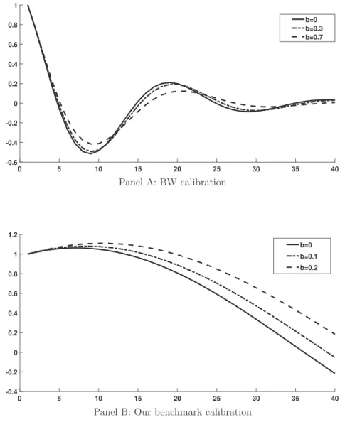
When b is increased further, however, the indetermi-nacy area progressively shrinks, due to a quantitatively significant downward shift in the Hopf bifurcation locus.

InFig. 11, we display the Impulse Response Functions of output to a positive sunspot shock when the value of b is progressively increased, considering two alternative calibrations for the other structural parameters. The initial BW calibration with

ε

cc

=

σ =

1

andΘ

=

0

.

11 (see Panel A), and our benchmark calibration with

ε

cc

=

2

.

3

, σ =

3 and Θ

=

0

.

16 (see Panel B). In the first

case, we increase b from 0 to 0.7, since the model remains in the indeterminacy area for this whole set of values. In the second case, we increase b from 0 to 0.3, since the model is no longer indeter-minate for large values of b under this calibration. As can be seen, in both cases, the effects are quantitatively marginal: an increase in b is associated with a slight increase in the persistence of output following a sunspot shock, but the hump-shaped dynamics is not getting closer to the data.

4.3.3. Dynamic learning by doing in production

We now experience with alternative specifications regarding the productive side of the economy, and consider as an example an enriched specification of the production function displaying dynamic learning by doing à laChang et al.(2002). The production function is now:

Yt

=

Af (utKt

,

Nt)e(u

¯

tK

¯

t

,

Nt) (4.1)

where Nt

=

xtltare hours worked by the representative household

in efficiency units, Ntbeing the aggregate (economy wide) average,

and xt is the skill level of this household. The latter accumulates

as:10 xt

=

x1 −φ t−1l φ t−1 (4.2)

with

φ ∈

(0

,

1

]

.

When

φ =

0

,

we recover our benchmark case with

xt

=

xt−1

=

x

,

i.e. skills are constant over time. The representative firm’s profit maximization problem yields the modified optimality condition for hours worked in efficiency units:

w

t

=

Af2(utKt

,

Nt)e(u

¯

tK

¯

t

,

Nt)

.

The representative household maximizes its expected in-tertemporal utility function subject to the modified budget con-straint kt+1

=

(

1

−

uγ_t

/γ )

kt

+

w

txtlt

+

rtutkt

−

ctand the skill

accumulation Eq.(4.2). Denoting by

ζ

t the Lagrange multiplier

associated to the latter equation, the first-order conditions with respect to ltand xtare:

B

v

′

(ℓ −

lt

) =

u ′ (ct)

w

txt

+

βφ

x1 −φ t lφ− 1 t Et

ζ

t+1

ζ

t

=

u ′ (ct)

w

tlt

+

β

(1

−

φ

)x −φ t lφtEt

ζ

t+1 while other optimality conditions are unchanged.

It turns out that with this specification, the model’s dynamic properties are drastically changed as soon as

φ

exceeds 0 by any significant amount. When

φ >

0

,

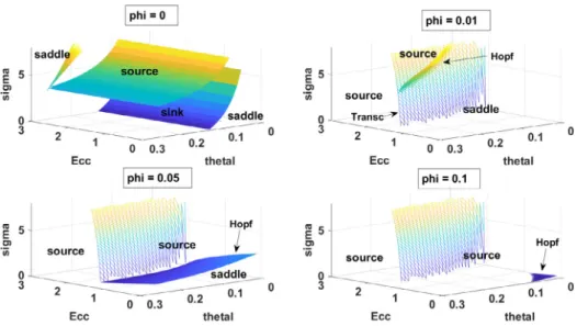
the model, reduced to its mini-mal dimension, involves 4 dynamic equations in 4 variables, among which two of them are state variables. As shown inFig. 12, when

φ =

0

.

01

,

the model features a Hopf and a transcritical bifurcation in the 3-dimensional plane defined by

ε

cc

, σ

and Θ

.

However,

the Hopf bifurcation is no longer associated with the existence of sunspot equilibria. Indeed, when

σ

crosses the Hopf bifurcation

10_{Chang et al.(2002) consider a non-constant returns-to-scale skill accumulation}

process. We rather choose a CRS specification to avoid adding too many additional parameters.

Fig. 11. Output dynamics following a positive sunspot shock for different values of b.

value

σ

H, the steady state switches from a saddle path to a source,

associated with locally unstable dynamics. Indeed, when

σ < σ

H

,

the model has two stable and two unstable eigenvalues. When

σ

crosses

σ

H

,

two (initially stable) complex conjugate eigenvalues

have a modulus crossing 1, and the steady-state becomes a source associated with four unstable eigenvalues.

The model also features a transcritical bifurcation. Starting from the area for which the steady state is a saddle, if

ε

cc is

increased until it crosses the transcritical bifurcation curve, one real eigenvalue crosses 1 and the steady state becomes a source associated with three unstable eigenvalues. If, on the other hand,

ε

ccis gradually increased starting from the area where the

steady-state is a source associated with four unstable eigenvalues, crossing the transcritical bifurcation locus implies that the model remains a source, but now associated with three unstable eigenvalues. In any case, indeterminacy is ruled out for any empirically credible values for

ε

cc

, σ

andΘ

.

Finally,Fig. 12shows that a similarly negative conclusion is ob-tained when larger values of

φ

are considered. The main difference is that the Hopf bifurcation curve progressively shifts downward (and eventually totally disappears) when

φ

increases, reducing the area for which the steady-state is a saddle path. Once again, indeterminacy is ruled out. Thus, introducing dynamic learning by doing in the production function does not appear to be a promising road to improve the model’s predictions because it tends to elimi-nate the possibility of existence of sunspot fluctuations.

At this stage, we are led to conclude that although the one-sector model with variable capital utilization rate is able to ex-plain crucial features of the estimated empirical responses of the economy to a standard demand shock, the model is not yet ready to survive a more stringent data confrontation. Other extensions and/or refinements to this model are necessary to improve the model’s predictions in this dimension. We leave this discussion for further research.

5. Conclusion

If one wants sunspot fluctuations based on self-fulfilling prophecies to be more credible, a requirement is that endogenous fluctuations models replicate the main stylized facts of a demand shock. Considering a generalized version of the BW model and allowing for more substitution between intertemporal consump-tion, a moderate increase in factor substitutability and a slightly higher degree of increasing returns, we have shown that, from a theoretical point of view, the one-sector stochastic growth model with variable capacity utilization is able to generate a hump-shaped dynamics of output in response to a pure sunspot shock. Yet, this response is too persistent for the model to be directly confronted to the data. Further research should be done in order to determine which extension of the model should be introduced to improve the results in this dimension. Dufourt et al. (2017) are exploring whether a two-sector stochastic growth model with

Fig. 12. Indeterminacy area for different values ofφ.

variable capacity utilization enables the model to come closer to the data.

Appendix

A.1. Proof ofProposition 1 A steady state is a 4-uple (k∗

_,

l∗

_,

u∗

_,

c∗ ) such that: Af1(u ∗ k∗

,

l∗)u∗e(u∗k∗

,

l∗)

=

1

−

β

(1

−

δ

∗ )

β

≡

θ

β

(A.1a) Af1(u∗k∗

,

l∗)u∗e(u∗k∗

,

l∗)

=

u∗γ −1 (A.1b) c∗

=

Af (u∗k∗

,

l∗)e(u∗k∗

,

l∗)

−

δ

∗k∗ (A.1c) B

v

′(

ℓ −

l∗)

=

Af2(u ∗ K∗

,

l∗)e(u∗K∗

,

l∗)u′(c∗)

.

(A.1d) Using(A.1a)and(A.1b), we find

u∗

=

(

γ

(1

−

β

)

β

(

γ −

1)

)

1/γ implying

δ

∗

=

(1

−

β

)

β

(

γ −

1)

.

After substitution of this expression into(A.1a), we find that there exists a normalized steady state with k∗

₌

l∗

₌

1 solution of Eq.(A.1a)if and only if A

=

A∗

with A∗

≡

θ

β

1 f1(u∗

,

1)u∗e(u∗

,

1) with

θ =

1

−

β

(1

−

δ

∗ ). Including A∗

in(A.1c)–(A.1d)and using the share s

=

s(u∗

,

1) of capital income, we find

c∗

=

θ −

s

βδ

β

s

,

θ

(1

−

s) s

=

B

v

′ (

ℓ −

1) u′_(c∗₎

.

It follows that (k∗

_,

l∗

_,

c∗ )

=

(1

,

1

,

(

θ −

s

βδ

∗ )

/

s

β

) is a normalized steady state solution of the system (A.1a)–(A.1d) if and only if

A

=

A∗ and B

=

B∗ with B∗

≡

θ

(1

−

s)u ′ (c∗ ) s

v

′₍

ℓ −

₁₎

.

□

A.2. Proof ofLemma 1

Eq.(2.12)can be written:

Af1(utKt

,

lt)ute(utKt

,

lt)

=

uγ −t 1

.

Solving this equation gives ut as a function of capital and labor,

namely ut

=

ν

(Kt

,

lt), which allows us to apply the implicit

function theorem to compute the following elasticities:

ε

νK(uK

,

l)

=

ν

1 (uK

,

l)k

ν

(uK

,

l)

=

−

1−_σs

+

ε

_eK

γ −

1

+

1−_σs

−

ε

_eK

,

ε

νl(uK

,

l)

=

ν

2(uK

,

l)l

ν

(uK

,

l)

=

1−s σ

+

ε

eL

γ −

1

+

1−_σs

−

ε

_eK

.

(A.2)

From(2.2)–(2.3)and recalling that Rt

=

1

−

δ

t

+

rtut, we also derive

at the steady state:

∂w

∂

K K

w

=

(1

+

ε

νK)

(ε

eK

+

s

σ

) ,

∂w

∂

l l

w

=

ε

el

−

s

σ

+

ε

νl

(ε

eK

+

s

σ

)

∂

R

∂

K K R

=

θ

(1

+

ε

νK)

(

ε

eK

−

1

−

s

σ

)

,

∂

R

∂

l l R

=

ε

el

+

1

−

s

σ

+

ε

νl

(

ε

eK

−

1

−

s

σ

)

.

(A.3)

We may then compute the following linearized system:

⎛

⎜

⎝

dKt+1 K∗ dlt+1 l∗

⎞

⎟

⎠

=

J

⎛

⎜

⎝

dKt K∗ dlt l∗

⎞

⎟

⎠

with J= ⎛ ⎝ 1 0 −J21 J22 1 J22 ⎞ ⎠ × ⎛ ⎝ J11 J12 −(1+ε_νK)(εeK+ s σ) − [ − 1 εlw +εeL− s σ +ενK(εeK+ s σ) ] ⎞ ⎠