Computational perception of physical object properties

Computational Perception of Physical Object Properties

by

Jiajun Wu

B.Eng., B.Ec., Tsinghua University (2014)

Submitted to the Department of Electrical Engineering and Computer Science in partial fulfillment of the requirements for the degree of

Master of Science at the

MASSACHUSETTS INSTITUTE OF TECHNOLOGY February 2016

@

Massachusetts Institute of Technology 2016. All rights reserved.

Signature redacted

Author ...

Department of E)rical Engineering and Computer Science January 29, 2016

Certified by

...

Signature redacted...

William T. Freeman Thomas and Gerd Perkins Professor of Electrical Engineering and Computer Science Thesis Supervisor

Signature redacted

C ertified by ... ...

Joshua B. Tenenbaum Professor of Computational Cognitive Science Thesis Supervisor

Signature redacted

A ccepted by ... ... U ---- -. . .. .. .. .. .. .. .. .. .

Leslie A. Kolodziejski

MASSACHUSMS INSTTUTE Chair, Depar ent Committee on Graduate Students OF TECHNOLOGY

APR

15 2016

LIBRARIES

Computational Perception of Physical Object Properties

by

Jiajun Wu

Submitted to the Department of Electrical Engineering and Computer Science on January 29, 2016, in partial fulfillment of the

requirements for the degree of Master of Science

Abstract

We study the problem of learning physical object properties from visual data. In-spired by findings in cognitive science that even infants are able to perceive a physical world full of dynamic content at a early age, we aim to build models to characterize object properties from synthetic and real-world scenes. We build a novel dataset con-taining over 17, 000 videos with 101 objects in a set of visually simple but physically rich scenarios. We further propose two novel models for learning physical object prop-erties by incorporating physics simulators, either a symbolic interpreter or a mature physics engine, with deep neural nets. Our extensive evaluations demonstrate that these models can learn physical object properties well and, with a physic engine, the responses of the model positively correlate with human responses. Future research directions include incorporating the knowledge of physical object properties into the understanding of interactions among objects, scenes, and agents.

Thesis Supervisor: William T. Freeman

Title: Thomas and Gerd Perkins Professor of Electrical Engineering and Computer Science

Thesis Supervisor: Joshua B. Tenenbaum

Acknowledgments

I would like to express sincere gratitude to my advisors, Professor William Freeman

and Professor Joshua Tenenbaum. Bill and Josh are always inspiring and encouraging, and have led me through my research with profound insights. Not only have they taught me how to aim for top-quality research, but they have been sharing with me invaluable lessons about life.

I deeply appreciate the guidance and support from my undergraduate advisor, Professor Zhuowen Tu, who introduced me into the world of AI and vision, and has long been my mentor and friend since then. I also thank Professor Andrew Chi-Chih Yao and Professor Jian Li for advising me during my undergraduate study, Dr. Yuandong Tian for mentoring me at Facebook AI Research, and Dr. Kai Yu and Dr. Yinan Yu for mentoring me at Baidu Research.

The thesis would not have been possible without the inspiration and support from my colleagues in the MIT Vision Group and Computational Cognitive Science (Co-CoSci) Group. I would like to deliver my appreciation to my collaborators, Dr. Joseph Lim, Tianfan Xue, and Dr. Ilker Yildirim. I am also thankful to other encouraging and helpful group members, especially Andrew Owens, Donglai Wei, Dr. Tomer Ull-man, Katie BouUll-man, Kelsey Allen, Tejas Kulkarni, Dr. Dilip Krishnan, Dr. Hossein Mohabi, Dr. Tali Dekel, Dr. Daniel Zoran, Pedro Tsividis, and Hongyi Zhang.

I would like to extend my appreciation to my dear friends for their backing in my

academic and daily life.

I received the Edwin S. Webster Fellowship during my first year, and have been

partially funded by NSF-6926677 (Reconstructive Recognition). I appreciate the sup-port from all funding agencies.

Contents

1 Introduction 13

2 Modeling the Physical World 17

2.1 Scenarios ... ... 18

2.2 The Physics 101 Dataset ... 20

3 Physical Object Model: Learning with a Symbolic Interpreter 23 3.1 Visual Property Discoverer . . . . 24

3.2 Physics Interpreter . . . . 25

3.3 Physical World Simulator . . . . 26

3.4 Experim ents . . . . 27

3.4.1 Learning Physical Properties . . . . 28

3.4.2 Detecting Objects with Unusual Properties . . . . 30

3.4.3 Predicting Outcomes . . . . 31

4 Physical Object Model: Incorporating a Physics Engine 35 4.1 The Galileo M odel . . . . 35

4.1.1 Tracking as Recognition . . . . 38

4.1.2 Inference . . . . 38

4.2 Sim ulations . . . . 38

4.3 Bootstrapping as Efficient Perception in Static Scenes . . . . 39

4.4 Experim ents . . . . 41

4.4.2 M ass Prediction . . . . 42 4.4.3 "Will it move" Prediction . . . . 43

5 Beyond Understanding Physics 45

List of Figures

2-1 Abstraction of the physical world, and a snapshot of our dataset. . 18

2-2 Illustrations of the scenarios in our Physics 101 dataset. . . . . 19 2-3 Physics 101: this is the set of objects we used in our experiments.

We vary object material, color, shape, and size, together with external conditions such as the slope of a surface or the stiffness of a string. Videos recording the motions of these objects interacting with target objects will be used to train our algorithm. . . . . 20

3-1 Our first model exploits the advancement of machine learning algo-rithm (convolutional neural network) - we supervise all levels by a

physics interpreter. This interpreter provides the physical constraints

on what each layer can take values. During the training and testing, our model has no label of physical properties, in contrast to the stan-dard approaches. . . . . 24

3-2 Charts for the estimations of rings. The physical properties, especially density, of the first ring is different from those of the other rings. The difference is hard to perceive by merely visual appearances; however, by observing videos with object interactions, our algorithm is able to learn the properties and find the outlier. All figures are on a log-normalized scale. . . . . 30 3-3 Heat maps of user predictions, model outputs (in orange), and ground

truths (in white). Objects from top to bottom, left to right: dough, metal coin, metal pole, plastic block, plastic doll, and porcelain. . . . 31

4-1 Our second model formalizes a hypothesis space of physical object rep-resentations, where each object is defined by its mass, friction coef-ficient, 3D shape, and a positional offset w.r.t. an origin. To model videos, we draw objects from that hypothesis space into the physics engine. The simulations from the physics engine are compared to ob-servations in the velocity space. . . . . 36

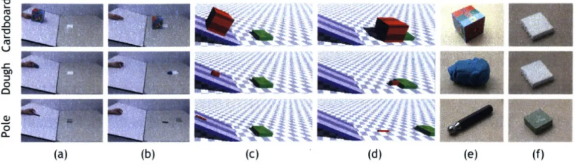
4-2 Simulation results. Each row represents one video in the data: (a) the first frame of the video, (b) the last frame of the video, (c) the first frame of the simulated scene generated by Bullet, (d) the last frame of the simulated scene, (e) the estimated object with larger mass, (f) the

estuimateu oUjecUtwih larig iiction cIeUfIcIent. . . . . 39 4-3 Mean squared errors of oracle estimation, our estimation, and uniform

estimations of mass on a log-normalized scale, and the correlations between estimations and ground truths . . . . 41 4-4 The log-likelihood traces of several chains with and without

recognition-model (LeNet) based initializations. . . . . 41 4-5 Mean errors in numbers of pixels of human predictions, Galileo

out-puts, and a uniform estimate calculated by averaging ground truth ending points over all test cases. As the error patterns are similar for both target objects (foam and cardboard), the errors here are averaged across target objects for each material. . . . . 43 4-6 Heat maps of user predictions, Galileo outputs (orange crosses), and

ground truths (white crosses). . . . . 43 4-7 Average accuracy of human predictions and Galileo outputs on the

tasks of mass prediction and "will it move" prediction. Error bars indicate standard deviations of human accuracies. . . . . 44

List of Tables

3.1 Accuracies

(%,

for oracle) or clustering purities

(%,

for joint training) on material estimation. In the joint training case, as there is no su-pervision on the material layer, it is not necessary for the network to specifically map the responses in that layer to material labels, and we do not expect the numbers to be comparable with the oracle case. Our analysis is just to show even in this case the network implicitly grasps some knowledge of object materials. . . . . 29 3.2 _{Correlation coefficients of our estimations and ground truth for mass,}

density, and volume . . . . 30 3.3 Mean squared errors in pixels of human predictions (H), model outputs

(M), or uniform estimate minimizing the mean squared error (U) . . . 31

3.4 Correlation coefficients on the tasks of predicting the moving distance and the bounce height, and accuracies on predicting whether an object floats . . . . 32

4.1 Correlations between pairs of outputs in the mass prediction experi-ment (in Spearman's coefficient) and in the "will it move" prediction experiment (in Pearson's coefficient). . . . . 44

Chapter 1

Introduction

Our visual system is designed to perceive a physical world that is full of dynamic content. Consider yourself watching a Rube Goldberg machine unfold: as the kinetic energy moves through the machine, you may see objects sliding down ramps, collid-ing with each other, rollcollid-ing, entercollid-ing other objects, fallcollid-ing - many kinds of physical interactions between objects of different masses, materials, and other physical proper-ties. How does our visual system recover so much content from the dynamic physical world? What is the role of experience in interpreting a novel dynamical scene?

Further, there is evidence that babies form a visual understanding of basic physical concepts, as a basic component of common sense knowledge, at a very young age; they learn properties of objects from their motions [1]. As young as 2.5 to 5.5 months old, infants learn basic physics even before they acquire advanced high-level knowledge like semantic categories of objects [5, 1]. Both infants and adults also use their physics knowledge to learn and discover latent labels of object properties, as well as predict the physical behavior of objects [2]. These facts suggest the importance for a visual system of understanding physics, and motivate our goal of building a machine with such visual competency.

Recent behavioral and computational studies of human physical scene understand-ing push forward an account that people's judgments are best explained as proba-bilistic simulations of a realistic, but mental, physics engine [2, 151. Specifically, these studies suggest that the brain carries detailed but noisy knowledge of the physical

attributes of objects and the laws of physical interactions between objects (i. e., New-tonian mechanics). To understand a physical scene, and more crucially, to predict the future dynamical evolution of a scene, the brain relies on simulations from this mental physics engine.

Even though the probabilistic simulation account is very appealing, there are missing practical and conceptual leaps. First, as a practical matter, the probabilistic simulation approach is shown to work only with synthetically generated stimuli in only 2D or 3D block worlds. The joint inference of the mass and coefficient of friction is also not handled [2]. Second, as a conceptual matter, previous research rarely clarifies how a mental physics engine could take advantage of previous experience of the agent

118].

It is the case that humans have a life long experience with dynamical scenes, and a fuller account of human physical scene understanding should address it. We aim to build on the idea that humans utilize a realistic physics engine as part of a generative model to interpret real-world physical scenes. Given a video as observa-tion to the model, physical scene understanding in the model corresponds to inverting the generative model by probabilistic inference to recover the underlying physical ob-ject properties in the scene. Our formulation combines deep learning, which serves as a powerful low-level visual recognition system, with a physics simulator to estimate physical properties directly from unlabeled videos. We study two possible forms of a physics simulator: the first is a symbolic physics interpreter encoded as layers in deep learning; and the second is a mature physics engine. Compared to recent stud-ies in vision and robotics on predicting physical interactions for 3D reasoning [10, 231 and tracking [16], our goal is to infer physical object properties directly, and we in-corporate a generative physics simulator with a powerful discriminative recognition model, which distinguishes our framework from previous methods introduced in the computer vision and robotics community for predicting physical interactions or prop-erties of objects for various purposes [14, 20, 10, 23, 19, 3, 4, 8, 24].

We also construct a video dataset for evaluating machine and human performance on real-world data. We collected a dataset of 101 objects made of different materials and with a variety of masses and volumes. We started by collecting videos of these

objects from multiple viewpoints in four various scenarios: objects slide down an inclined surface and possibly collide with another object; objects fall onto surfaces made of different materials; objects splash in water; and objects hang on a spring. These seemingly straightforward setups require understanding multiple physical prop-erties, e.g., material, mass, volume, density, coefficient of friction, and coefficient of restitution, as discussed later. We called this dataset Physics101, highlighting that we are learning elementary physics, while also indicating the current object count. Our dataset contains not only over 12, 000 RGB videos, but also more than 4, 000 depth videos and audios, which could benefit our future study on learning from multi-modality data.

Based on the estimates we derived from visual input with a physics simulator, a natural extension is to generate or synthesize training data for any automatic learning systems by bootstrapping from the videos already collected, and labeling them with estimates of models. This is a self-supervised learning algorithm for inferring generic physical properties, and relates to the wake/sleep phases in Helmholtz machines [9], and to the cognitive development of infants. Extensive studies suggest that infants either are born with or can learn quickly physical knowledge about objects when they are very young, even before they acquire more advanced high-level knowledge like semantic categories of objects [5, 1]. Young babies are sensitive to physics of objects mainly from the motion of foreground objects from background [1]; in other words, they learn by watching videos of moving objects. But later in life, and clearly in adulthood, we can perceive physical attributes in just static scenes without any motion.

Here, building upon the idea of Helmholtz machiness [9], our approach suggests one potential computational path to the development of the ability to perceive physical content in static scenes. Following the recent work [22], we train a recognition model

(i.e., sleep cycle) that is in the form of a deep convolutional network, where the

training data is generated in a self-supervised manner by the generative model itself

(i.e., wake cycle: real-world videos observed by our model and the resulting physical

with a relatively reliable mental physics engine, or acquires it soon after birth. Our research has various generalizations and extensive applications. With physical object properties, we may build intelligent systems for high-level scene understanding, including the study of physics-related concepts like object stability in the scene, and we may incorporate agents interacting with the physical world for particular goals. Our study is inspired by findings in developmental psychology, but can also lead to interesting and fundamental research questions there, for instance, whether there exist connections between the learning processes of infants and machines on physical concepts.

Chapter 2

Modeling the Physical World

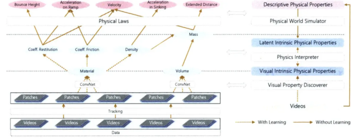
There exist highly involved physical processes in daily events in our physical world, even simple scenarios like objects sliding down an inclined surface. As shown in Figure 2-la, we can divide all involved physical properties into two groups: the first is the intrinsic physical properties of objects like volume, material, and mass, many of which we cannot directly measure from the visual input; the second is the descriptive physical properties which characterize the scenario in the video, including but not limited to velocity of objects, distances that objects traveled, or whether objects float if they are thrown into water. The second group of parameters are observable, and are determined by the first group, while both of them determine the content in videos. Our goal is to build an architecture that can automatically discover those observ-able descriptive physical properties from unlabeled videos, and use them as supervi-sion to further learn and infer unobservable latent physical properties. Our generative model can then apply learned knowledge of physical object properties for other tasks like predicting outcomes in the future.

The computer vision community has made much progress through its datasets, and there are datasets of objects, attributes, materials, and scene categories. Here, we introduce a new type of dataset, Physics 101, capturing physical interactions of objects. The dataset consists of four different scenarios, for each of which plenty of intriguing questions may be asked. For example, in the ramp scenario, will the object on the ramp move, and if so and two objects collide, which of them will move next

Descriptive Physical Properties

Acceleration

Velocity Bounce Extended

Height Distance

Intrinsic Physical Object Properties

Coeff Coeff Restitution Friction Mass

Material Volume

Videos

(a) Abstraction of physical prop-erties and how they determine the content of video.

(b) Our scenario and a snapshot of our dataset,

Physics 101, of various objects at different stages. Our data are taken by four sensors (3 RGB and 1 depth).

Figure 2-1: Abstraction of the physical world, and a snapshot of our dataset.

and how far?

2.1

Scenarios

We seek to learn physical properties of objects by observing videos. To this end, we build a dataset by recording videos of moving objects. We pick an introductory setup with four different scenarios, which are illustrated in Figures 2-1b and 2-2. We then introduce each scenario in detail.

Ramp We put an object on an inclined surface, and the object may either slide

down or keep static, due to gravity and friction. This seemingly straightforward scenario already involves understanding many physical object properties including material, coefficient of friction, mass, and velocity. Figure 2-2a analyzes the physics behind our setup.

At first, there are three external forces on the object: a gravitational force G, a normal force N from the surface, and a friction force R. When the friction force R

is strong, then the object would not move. Otherwise, the object will start to slide. After it reaches the ground, these forces would still exist, but now the object will slow

R., N,

NH 1N N, NB N N

I. Initial setup II. Before collision III. At collision IV. After collision V. Final result

(a) The ramp scenario. Several physical properties will determine if object A will move, if it will reach to object B, and how far each object will move. Here, N, R, and G indicate a normal force, a friction force, and a gravity force, respectively.

I. Initial setup II. After extension I. A floating object II. A sunk object (b) The spring scenario. (c) The liquid scenario.

I. Initial setup II. At collision III. Bounce (d) The fall scenario.

Figure 2-2: Illustrations of the scenarios in our Physics 101 dataset.

down due to the friction force R. If the object A slides all the way to B, then A will

hit B and both of them will move. How far A and B move depends on their friction coefficients, masses, and the velocity of A at the moment of collision.

In this scenario, the observable descriptive physical properties are the velocities of the objects, and the distances both objects traveled. The latent properties directly involved are coefficient of friction and mass.

Spring We hang objects on a spring, and gravity on the object will stretch the

spring, as shown in Figure 2-2b. Here the observable descriptive physical property is length that the spring gets stretched, and the latent properties are the mass of the

object and the elasticity of the spring.

Fall We drop objects in the air, and they freely fall onto various surfaces. Figure 2-2d illustrates this scenario. Here the observable descriptive physical properties are

Plastic Block Foam Hallow Wood Metal Pole Wooden Pole Plastic Doll Wooden Bleck Hollow% Rubbe, Cardlbomii

*

4 eE

VOO

Metal Coin Dough Plastic O Toy

-

Porcelain Plastic -10000

4l

40

1111146

IWO.1

, 10

0 Rubber #4

V

Target I

Figure 2-3: Physics 101: this is the set of objects we used in our experiments. We vary object material, color, shape, and size, together with external conditions such as the slope of a surface or the stiffness of a string. Videos recording the motions of these objects interacting with target objects will be used to train our algorithm.

the the bounce heights of the object, and the latent properties are the coefficient of restitution of the object and the surface.

Liquid As shown in Figure 2-2c, we drop objects into some liquid, and they may

float or sink at various speeds. In this scenario, the observable descriptive physical property is the velocity of the sinking object (0 if it floats), and the latent properties are the densities of the object and the liquid.

2.2

The Physics 101 Dataset

The outcomes of various physical events depend on multiple factors of objects, such as materials (density and friction coefficient), sizes and shapes (volume), and slopes of ramps (gravity), elasticities of springs, etc. We collect our dataset while varying all these conditions. Figure 2-3 shows the entire collection of our 101 objects, and the following are more details about our variations:

Material Our 101 objects are made of 15 different materials - cardboard, dough, foam, hollow rubber, hollow wood, metal coin, metal pole, plastic block, plastic doll, plastic ring, plastic toy, porcelain, rubber, wooden block, and wooden pole.

Appearance _{For each material, we have 4 ~ 12 objects of different sizes, shapes,} and colors.

Slope (ramp) We also vary the angle a between the inclined surface and the ground

(to vary the gravity force). We set a = 100 and 200 for each object.

Target (ramp) We have two different target objects - a cardboard and a foam box. They are made of different materials, thus having different friction coefficients and densities.

Spring We use two springs with different stiffness.

Surface (fall) _{We drop objects onto five different surfaces: foam, glass, metal,}

wooden table, and woolen rug. These materials have different coefficients of restitu-tion.

We also measure the physical properties of these objects. We record the mass and volume of each object, which also determine density. Please refer to the supplementary material for the statistics of all these measured properties.

For each setup, we record their actions for 3 ~ 10 trials. We measure multiple times because some external factors, e.g., _{orientations of objects and rough planes,}

may lead to different outcomes. Having more than one trial per condition increases the diversity of our dataset by making it cover more possible outcomes.

Finally, we record each trial from three different viewpoints: one sideview, one top-down view, and one upper-top view. For the first two views, we take data with DSLR cameras, and for the upper-top view, we use a Kinect V2 to record both RGB and depth maps. After removing trials with significant noise, we have 4,352 trials in total. Given we captured videos in three RGB maps and one depth map, there are

Chapter 3

Physical Object Model: Learning

with a Symbolic Interpreter

We aim to discover physical object properties under a unified system with minimal supervision, rather than training each classifier/regressor for labels (such as material and volume) in a fully supervised manner. With this philosophy, we develop two physical object models; one uses deep learning and a symbolic physics interpreter for recognizing physical properties, and the other incorporates a mature physics engine and predicts physical properties via an analysis-by-synthesis approach. Both meth-ods have built-in knowledge of physics, and work in an unsupervised setting. With these generative models, we are able to not only discover all physical properties (e.g. material, volume) simply by observing motions of objects in unlabeled videos, but also predict different physical interactions (e.g. how far will the object move, if it moves at all) based on inferred physical properties.

In this chapter we describe our first model, shown in Figure 3-1. Our method is based on a convolutional neural network (CNN) [11], which consists of three compo-nents. The bottom component is a visual property discoverer, which aims to discover physical properties like material or volume which could at least partially be observed from visual input; the middle component is a physics interpreter, which explicitly encodes physical laws into the network structure and models latent physical proper-ties like density and mass; the top component is a physical world simulator, which

Bounce Height Acceleraton _{on ampn} Velocity Acceleraton _{in Sinken} Extended Distance Descriptive Physical Properties Physical Laws Physical World Simulator

Mass

Latent Intrinsic Physical Properties

Coeff Restitution Coeff Friction Density

Physics Interpreter

Material Volume Visual Intrinsic Physical Properties

ConvNet ConvNet Visual Property Discoverer

Videos

With Learning Without Learning

Data

Figure 3-1: Our first model exploits the advancement of machine learning algorithm (convolutional neural network) - we supervise all levels by a physics interpreter. This interpreter provides the physical constraints on what each layer can take values. Dur-ing the trainDur-ing and testDur-ing, our model has no label of physical properties, in contrast to the standard approaches.

characterizes descriptive physical properties like distances that objects traveled, all of which we may directly observe from videos.

Our network corresponds to our physical world model introduced in Chapter 2. We would like to emphasize here that our model learns object properties from completely unlabeled data. We do not provide any labels for physical properties like material, velocity, or volume; instead, our model automatically discovers observations from videos, uses them as supervision to the top physical world simulator, which in turn advises what the physics interpreter should discover.

3.1

Visual Property Discoverer

The bottom meta-layer of our architecture in Figure 4-1 is designed to discover and predict low-level properties of objects including material and volume, which can also be at least partially perceived from the visual input. These properties are the basic parts of predicting any derived physical properties at upper layers, e.g. density and mass.

first locate objects inside videos. We use a KLT point tracker [17] to track moving objects . We also compute a general background model for each scenario to locate foreground objects. Image patches of objects are then supplied to our visual property discoverer.

Material and volume Material and volume are properties that can be estimated directly from image patches. Hence, we have LeNet [12] on top of image patches extracted by the tracker. Once again, rather than directly supervising each LeNet with their labels, we supervise them by automatically discovered observations which are provided to our physical world simulator. To be precise, we do not have any individual loss layer for LeNet components. Note that inferring volumes of objects from static images is an ambiguous problem. However, this problem is alleviated by our data from different viewpoints and both RGB and depth maps.

3.2

Physics Interpreter

The second meta-layer of our model is designed to encode the physical laws. For instance, if we assume an object is homogeneous, then its density is determined by its material; the mass of an object should be the multiplication of its density and volume. Based on material and volume, we expand a number of physical properties in this physics interpreter, which will later be used to connect to real world observations.

The following shows how we represent each physical property as a layer depicted in Figure 4-1:

Material A Nm dimensional vector, where Nm is the number of different materials.

The value of each dimension represents the confidence that the object belongs to that dimension. This is an output of our visual property discoverer.

Volume A scalar representing the predicted volume of the object. This is an output

of our visual property discoverer.

Coefficient of friction and density Each is a scalar representing the predicted physical property based on the output of the material layer. Each output is the inner

product of Nm learned parameters and responses from the material layer.

Coefficient of restitution A Nm dimensional vector representing how much of the

kinetic energy remains after a collision between the input object with other objects of various materials. The representation is a vector, not a scalar, as the coefficient of restitution is determined by the materials of both objects involved in the collision. Mass A scalar representing the predicted mass based on the outputs of the density layer and the volume layer. This layer is the product of the density and volume layers.

3.3

Physical World Simulator

Our physical world simulator connects the inferred physical properties to real-world observations. We have different observations for different scenarios, and use velocities of objects and distances objects traveled as observations of the ramp sce-nario, the length that the string is stretched as an observation of the spring scesce-nario, the bounce distance as an observation of the fall scenario, and the velocity that object sinks as an observation of the liquid scenario. All observations can be derived from the output of our tracker.

To connect those observations to physical properties our model inferred, we employ physical laws. The physical laws we used in our model include

Newton's law F = mg sin 0 - pmg cos 0 = ma, or (sin 0 - p cos O)g = a, where 0 is

angle between the inclined surface and the ground, p is the coefficient of friction, and

a is the acceleration of an object (observation). This is used for the ramp scenario.

Conservation of momentum and energy CR = (Vb - Va)/(ta - Ub), where vi

is the velocity of object i after collision, and ui is its velocity before collision. All ui and vi are observations, and this is also used for the ramp scenario.

Hooke's law F = kX, where X is the distance that the string is extended (our

observation), k is the stiffness of the string, and F = G = mg is the gravity on the object. This is used for the spring scenario.

Bounce CR= h/H, where CR is the coefficient of restitution, h is the bounce height (observation), and H is the drop height. This can be viewed as another representation of conservation of energy and momentum, and is used for the fall scenario.

Buoyancy dVg - dmVg = ma = dVa, or (d - d.)g = da, where d is density of the object, d, is the density of water (constant), and a is the acceleration of the object in water (observation). Note that for d < de, a = 0. This is used for the liquid scenario.

We use MSE between our model's estimate and the target value supplied by the physical world simulator as our loss during training.

3.4

Experiments

In this section, we present experiments with our models in various settings. We start with extensive verifications of our models on learning physical properties. Later, we investigate the generalization ability of our model on other tasks like detecting objects with unusual properties, predicting outcomes given partial information, and transferring knowledge across different scenarios. We use Torch7 [6] for all experi-ments.

For learning physical properties from Physics 101, we study our algorithm in the following settings:

" Split by frame: for each trial of each object, we use 95% of the patches we get from tracking as training data, while the other 5% of the patches as test data.

" Split by trial: for each trial of each object, we use all patches in 95% of the trials we have as training data, while patches in the other 5% of the trials as test data.

" Split by object: we randomly choose 95% of the objects, and use their patches as training data and the others as test data.

Among these three settings, split by frame is the easiest as for each patch in test data, the algorithm may find some very similar patch in the training data. Split by

object is the most difficult setting as it requires the model to generalize to objects that it has never seen before.

We consider training our model in different ways:

" Oracle training: we train our model with images of objects and their associated

ground truth labels. We apply oracle training on those properties we have ground truths labels of (material, mass, density, and volume).

" Standalone training: we train our model on data from one scenario. Automat-ically extracted observations serve as supervision.

* Joint training: we

jointly

train the entire network

on

all training data without any labels of physical properties. Our only supervision is the physical laws encoded in the top physical world simulator. Data from different scenarios supervise different layers in the network.

Oracle training is designed to test the ability of each component and can be viewed as an upper bound of the performance the model may achieve. Our focus is on standalone and joint training, where our model learns from unlabeled videos directly.

We are also interested in understanding how our model can perform at inferring some physical properties purely from depth maps. Therefore, besides using RGB data, we conduct some experiments where training and test data are depth maps only.

3.4.1

Learning Physical Properties

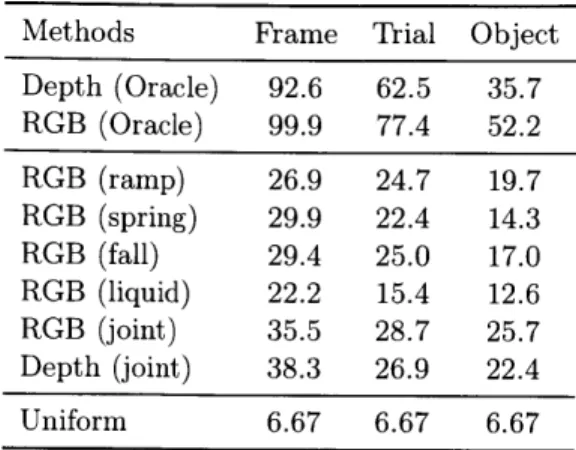
Material perception: We start with the task of material classification. Table 3.1

shows the accuracy of the oracle models on material classification. We observe that they can achieve nearly perfect results in the easiest case, and is still significantly better than chance on the most difficult split-by-object setting. Both depth maps and RGB maps give good performance on this task with oracle training.

Methods Frame Trial Object Depth (Oracle) 92.6 62.5 35.7 RGB (Oracle) 99.9 77.4 52.2 RGB (ramp) 26.9 24.7 19.7 RGB (spring) 29.9 22.4 14.3 RGB (fall) 29.4 25.0 17.0 RGB (liquid) 22.2 15.4 12.6 RGB (joint) 35.5 28.7 25.7 Depth (joint) 38.3 26.9 22.4 Uniform 6.67 6.67 6.67

Table 3.1: Accuracies (%, for oracle) or clustering purities (%, for joint training) on material estimation. In the joint training case, as there is no supervision on the material layer, it is not necessary for the network to specifically map the responses in that layer to material labels, and we do not expect the numbers to be comparable with the oracle case. Our analysis is just to show even in this case the network implicitly grasps some knowledge of object materials.

In the standalone and joint training case, given we have no labels on materials, it is not possible for the model to classify materials; instead, we expect it to cluster objects by their materials. To measure this, we perform K-means on the responses of the material layer of test data, and use purity, a common measure for clustering, to measure if our model indeed discovers clusters of materials automatically. As shown in Table 3.1, the clustering results indicate that the system learns the material of objects to a certain extent.

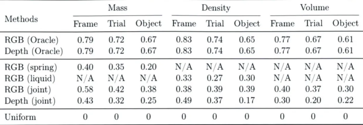
Physical parameter estimation: We then test our systems, trained with or

with-out oracles, on the task of physical property estimation. We use Pearson product-moment correlation coefficient as measures. Table 4-3 shows the results on estimating mass, density, and volume. Notice that here we evaluate the outputs on a log scale to avoid unbalanced emphases on objects with large volumes or masses.

We observe that with oracle our model can learn all physical parameters well. For standalone and joint learning, our model is also consistently better than a nontrivial baseline, which selects the optimum uniform estimate which minimizes the mean squared error.

Mass Density Volume

Methods Frame Trial Object Frame Trial Object Frame Trial Object

RGB (Oracle) 0.79 0.72 0.67 0.83 0.74 0.65 0.77 0.67 0.61

Depth (Oracle) 0.79 0.72 0.67 0.83 0.74 0.65 0.77 0.67 0.61

RGB (spring) 0.40 0.35 0.20 N/A N/A N A N A N/A N1A

RGB (liquid) N A N/A N'A 0.33 0.27 0.30 N A N A N 'A RGB (joint) 0.58 0.42 0.38 0.38 0.39 0.39 0.40 0.37 0.30

Depth (joint) 0.43 0.32 0.25 0.49 0.37 0.17 0.30 0.20 0.22

Uniform 0 0 0 0 0 0 0 0 0

Table 3.2: Correlation density, and volume

Mass Density

a CT e a b c d a

Est Est

coefficients of our estimations and ground truth for mass,

Volume

Est

a b C d e

Figure 3-2: Charts for the estimations of rings. The physical properties, especially density, of the first ring is different from those of the other rings. The difference is hard to perceive by merely visual appearances; however, by observing videos with object interactions, our algorithm is able to learn the properties and find the outlier.

All figures are on a log-normalized scale.

3.4.2

Detecting Objects with Unusual Properties

Sonetimes objects with similar appearances may have distinct physical properties. In this section, we test whether our system is able to find these expectation-violation cases.

In Physics 101, among all five plastic rings, the bottom part of smallest ring is made of a different material with a larger density, which makes its mass greater than those of the other four, but its volume smaller. The material of the smallest ring also has a lower friction coefficient, indicating that the velocity of the smallest ring at collision would be higher than those of the others.

In Figure 3-2, we show the estimations of our RGB joint model on the properties of all five rings, as well as their appearances. As shown, it is hard to perceive the difference between the physical properties of the first ring and those of the others

Material Cardboard Foam H M U H M U cardboard 28.8 40.7 97.0 15.0 77.2 84.0 dough 27.4 25.2 84.4 150.9 105.1 113.4 hollow wood 35.7 19.4 108.9 81.0 35.0 21.4 metal coin 13.4 32.2 149.8 31.9 33.3 75.8 metal pole 272.9 257.6 280.0 91.4 188.7 184.0 plastic block 29.8 82.1 97.6 46.9 57.2 35.0 plastic doll 49.4 23.6 44.0 128.8 41.8 93.9 plastic toy 30.1 41.9 121.2 33.3 9.5 70.6 porcelain 138.5 127.0 110.9 196.0 216.6 314.8 wooden block 45.9 32.8 36.2 47.3 37.5 14.2 wooden pole 78.9 88.0 138.9 58.7 89.8 74.3 Mean 68.2 70.1 115.4 80.1 81.1 98.3

Table 3.3: M\ean squared errors in pixels of human predictions (H), model outputs (M), or uniform estimate minimizing the mean squared error (U)

Figure 3-3: Heat maps of user predictions, model outputs (in orange), and ground truths (in white). Objects from top to bottom, left to right: dough, metal coin, metal pole, plastic block, plastic doll, and porcelain.

purely from visual appearances. By observing videos where they slide down and hit other objects, our system can learn physical parameters, and model the outliers.

3.4.3

Predicting Outcomes

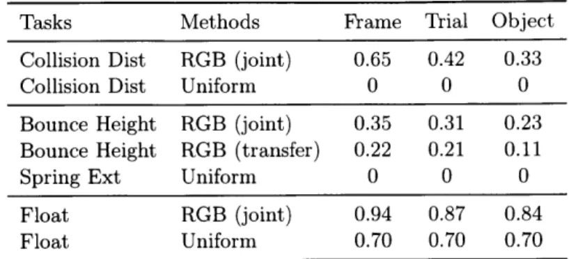
We may apply our model to a variety of outcome prediction tasks for different scenarios. We consider three of them: how far would an object move after being hit

by another object; how high an object will bounce after being dropped at a certain

height; and whether an object will float in the water. With estimated physical object properties, our model can answer these questions using physical laws.

Transferring Knowledge Across Multiple Scenarios As some physical edge is shared across multiple scenarios, it is natural to evaluate how learned

knowl-Tasks Methods Frame Trial Object Collision Dist RGB (joint) 0.65 0.42 0.33

Collision Dist Uniform 0 0 0

Bounce Height RGB (joint) 0.35 0.31 0.23

Bounce Height RGB (transfer) 0.22 0.21 0.11

Spring Ext Uniform 0 0 0

Float RGB (joint) 0.94 0.87 0.84

Float Uniform 0.70 0.70 0.70

Table 3.4: Correlation coefficients on the tasks of predicting the moving distance and the bounce height, and accuracies on predicting whether an object floats

edge from one scenario may be applied to a novel one. Here we consider the case where the model is trained on all but the fall scenarios. We then apply the model to the fall scenario for predicting how high an object bounces. Our intuition is the learned coefficients of restitution from the ramp scenario can help to predict to some extent.

Results Table 3.4 shows outcome prediction results. We can see that our method works well, and can also transfer learned knowledge across multiple scenarios.

Behavior Experiments We would like to see how well our model does compared to a human. To do this, we conducted experiments on predicting the moving distance of

an object after collision on Amazon Mechanical Turk. Specifically, among all objects that slide down, we select one object of each material, show AMT workers the videos of the object, but only to the moment of collision. We then ask workers to label where they believe the target object (either cardboard or foam) will be after the collision,

i.e., how far the target will move. Before testing, each users are provided four full

videos of other objects made of the same material, which contain complete collisions, so that users can simply infer the physical properties associated with the material and the target object in their mind. We tested 30 users per case.

Table 3.3 shows the mean squared errors in pixels of human predictions (H), model predictions (M), or uniform estimate minimizing the mean squared error (U). We can

see that the performance of our model is close to that of human on this task. Figure

3-3 shows the heat maps of user predictions, model outputs (orange), and ground truths (white).

Chapter 4

Physical Object Model:

Incorporating a Physics Engine

4.1

The Galileo Model

Here we describe our second model. Compared to the first one, our second model (shown in Figure 4-1) incorporates a physics engine in its core, and the gist of our second model can be summarized as probabilistically inverting the physics engine to recover unobserved physical properties of objects. For this model, we focus on the ramp scenario, and in honor of the famous physicist, we name our model Galileo.

The first component of Galileo is the physical object representations, where each object is a rigid body and represented not only by its 3D geometric shape (or volume) and its position in space, but also by its mass and its friction. All of these object attributes are treated as latent variables in the model, and are approximated or estimated on the basis of the visual input.

Specifically, we collectively refer to the unobserved latent variables of an object as its physical representation T. For each object i, T consists of its mass mi, friction coefficient ki, 3D shape Vi, and position offset pi w.r.t. an origin in 3D space.

We place uniform priors over the mass and the friction coefficient for each object: mi ~ Uniform(O.001, 1) and ki ~ Uniform(0, 1), respectively. For 3D shape Vi, we have four variables: a shape type ti, and the scaling factors for three dimensions

Physical object i - Mass (m) - Friction coefficient (k) - 3D shape (S) - Position offset (x) Draw two 7 physical objects 2 3D Physics engine Simulated velocities(t,_{1 v2}) Likelihood function Observed velocities (!r v.2) _,,_- Tra~cking algorithm

Figure 4-1: Our second model formalizes a hypothesis space of physical object

rep-resentations, where each object is defined by its mass, friction coefficient, 3D shape, and a positional offset w.r.t. an origin. To model videos, we draw objects from that hypothesis space into the physics engine. The simulations from the physics engine are compared to observations in the velocity space.

xi, yi, zi. We simplify the possible shape space in our model by constraining each

shape type ti to be one of the three with equal probability: a box, a cylinder, and a torus. Note that applying scaling differently on each dimension to these three basic shapes results in a large space of shapes.' The scaling factors are chosen to be uniform over the range of values to capture the extent of different shapes in the dataset.

Remember that our scenario consists of an object on the ramp and another

on the ground. The position offset, pi, for each object is uniform over the set

{0, 1, 2, . 5 , 5}. This indicates that for the object on the ramp, its position

can be perturbed along the ramp (i.e., in 2D) at most 5 units upwards or downwards

from its starting position, which is 30 units upwards on the ramp from the ground. The next component of our generative model is a fully-fledged realistic physics 'For shape type box, xi, y, and zi could all be different values; for shape type torus, we con-strained the scaling factors such that xi = zi; and for shape type cylinder, we concon-strained the scaling factors such that yi = zi.

engine that we denote as p. Specifically we use the Bullet physics engine

[7]

following the earlier related work. The physics engine takes a specification of each of the physical objects in the scene within the basic ramp setting as input, and simulates it forward in time, generating simulated velocity vectors for each object in the scene,

v., and v,2 respectively - among other physical properties such as position, rendered

image of each simulation step, etc.

In light of initial qualitative analysis, we use velocity vectors as our feature rep-resentation in evaluating the hypothesis generated by the model against data. We employ a standard tracking algorithm (KLT point tracker [17]) to "lift" the visual observations to the velocity space. That is, for each video, we first run the tracking algorithm, and we obtain velocities by simply using the center locations of each of the tracked moving objects between frames. This gives us the velocity vectors for the object on the ramp and the object on the ground, v,1 and v0 2, respectively. Note that

we could replace the KLT tracker with state-of-the-art tracking algorithms for more complicated scenarios.

The third part of Galileo is the likelihood function. We evaluate the observed real-world videos with respect to the model's hypotheses using the velocity vectors of objects in the scene. Given a pair of observed velocity vectors, v0, and v02, the

recovery of the physical object representations T and T2 for the two objects via

physics-based simulation can be formalized as

P(T, T2vI0 1, v02, p()) oc P(vO, v0 21v5I, 82) ' P(v8 1, V8 21T1, T2, p(.)) .P(T1, T2), (4.1)

where we define the likelihood function as P(vO, V_{0 2} 1v₈₁I, V82) = N(voIv, E), where vo

is the concatenated vector of vol, v0 2, and v, is the concatenated vector of v,1, V82. The

dimensionality of vo and v, are kept the same for a video by adjusting the number of simulation steps we use to obtain v, according to the length of the video. But from video to video, the length of these vectors may vary. In all of our simulations, we fix

E to 0.05, which is the only free parameter in our model. Experiments show that the

4.1.1

Tracking as Recognition

The posterior distribution in Equation 4.1 is intractable. In order to alleviate the burden of posterior inference, we use the output of our recognition model to predict and fix some of the latent variables in the model.

Specifically, we determine the Vi, or {ti, xi, yi, zi

},

using the output of the tracking algorithm, and fix these variables without further sampling them. Furthermore, we fix values of pis also on the basis of the output of the tracking algorithm.

4.1.2

Inference

Once

we initialize and fix

the

latent variables using the tracking algorithm as

our recognition model, we then perform single-site Metropolis Hasting updates on the remaining four latent variables, in, M2, k, and k2. At each MCMC sweep, we

propose a new value for one of these random variables, where the proposal distribution is Uniform(-0.05, 0.05). In order to help with mixing, we also use a broader proposal distribution, Uniform(-0.5, 0.5) at every 20 MCMC sweeps.

4.2

Simulations

For each video, as mentioned earlier, we use the tracking algorithm to initialize and fix the shapes of the objects, S1 and S2, and the position offsets, pi and

P2-We also obtain the velocity vector for each object using the tracking algorithm. P2-We determine the length of the physics engine simulation by the length of the observed video - that is, the simulation runs until it outputs a velocity vector for each object that is as long as the input velocity vector from the tracking algorithm.

We use 150 videos from our Physics 101 dataset, uniformly distributed across different object categories. We perform 16 MCMC simulations for a single video, each of which was 75 MCMC sweeps long. We report the results with the highest log-likelihood score across the 16 chains (i.e., the MAP estimate).

ra

On

0

(a) (b) (c) (d) (e) (f)

Figure 4-2: Simulation results. Each row represents one video in the data: (a) the

first frame of the video, (b) the last frame of the video, (c) the first frame of the

simulated scene generated by Bullet, (d) th e last frame of the simulated scene, (e) the estimated object with larger mass, (f) the estimated object with larger friction

coefficient.

of the top row shows the first and the last frame of a video, and the bottom row images show the corresponding frames from our model's simulations with the MAP estimate. We quantify different aspects of our model in the following behavioral experiments, where we compare our model against human subjects' judgments. Furthermore, we use the inferences made by our model here on the 150 videos to train a recognition model to arrive at physical object perception in static scenes with the model.

Importantly, note that our model can generalize across a broad range of tasks beyond the ramp scenario. For example, once we infer the coefficient friction of an object, we can make a prediction on whether it will slide down a ramp with a different slope by doing simulation. We test some of the generalizations in Chapter 4.4.

4.3

Bootstrapping as Efficient Perception in Static

Scenes

Based on the estimates we derived from the visual input with a physics engine, we bootstrap from the videos already collected, by labeling them with estimates

of Galileo. This is a self-supervised learning algorithm for inferring generic

wake/sleep phases in Helmholtz machines, and to the cognitive development of in-fants.

Here we focus on two physical properties: mass and friction coefficient. To do this, we first estimate these physical properties using the method described in earlier sections. Then, we train LeNet [13], a widely used deep neural network for small-scale datasets, using image patches cropped from videos based on the output of the tracker as data, and estimated physical properties as labels. The trained model can then be used to predict these physical properties of objects based on purely visual cues, even though they might have never appeared in the training set.

We also measure masses of all objects in the dataset, which makes it possible for us to quantitatively evaluate the predictions of the deep network. We choose one object per material as our test cases, use all data of those objects as test data, and the others as training data. We compare our model with a baseline, which always outputs a uniform estimate calculated by averaging the masses of all objects in the test data, and with an oracle algorithm, which is a LeNet trained using the same training data, but has access to the ground truth masses of training objects as labels. Apparently, the performance of the oracle model can be viewed as an upper bound

of our Galileo system.

Table 4-3 compares the performance of Galileo, the oracle algorithm, and the baseline. We can observe that Galileo is much better than baseline, although there is still some space for improvement.

Because we trained LeNet using static images to predict physical object properties such as friction and mass ratios, we can use it to recognize those attributes in a quick bottom-up pass at the very first frame of the video. To the extent that the trained LeNet is accurate, if we initialize the MCMC chains with these bottom-up predictions, we expect to see an overall boost in our log-likelihood traces. We test by running several chains with and without LeNet-based initializations. Results can be seen in Figure 4-4. Despite the fact that LeNet is not achieving perfect performance by itself, we indeed get a boost in speed and quality in the inference.

Mass

Methods _{MSE Corr}

Oracle 0.042 0.71 Galileo 0.052 0.44

Uniform 0.081 0

- initialization with recognition model - random initialization Oe+00 -0 o- le+05-o -2e+05 0 20 40 60 Number of MCMC sweeps

Figure 4-3: Mean squared errors of

or-acle estimation, our estimation, and Figure 4-4: The log-likelihood traces uniform estiniations of mass on a of several chains with and without log-normalized scale, and the correla- recognition-model (LeNet) based initial-tions between estimainitial-tions and ground izations.

truths

4.4

Experiments

In this section, we conduct experiments from multiple perspectives to evaluate our model. Specifically, we use the model to predict how far objects will move after the collision; whether the object will remain stable in a different scene; and which of the two objects is heavier based on observations of collisions. For every experiment, we also conduct behavioral experiments on Amazon Mechanical Turk so that we may compare the performance of human and machine on these tasks.

4.4.1

Outcome Prediction

In the outcome prediction experiment, our goal is to measure and compare how well human and machines can predict the moving distance of an object if only part of the video can be observed. Specifically, for behavioral experiments on Amazon Mechanical Turk, we first provide users four full videos of objects made of a certain material, which contain complete collisions. In this way, users may infer the physical properties associated with that material in their mind. We select a different object, but made of the same material, show users a video of the object, but only to the

moment of collision. We finally ask users to label where they believe the target object (either cardboard or foam) will be after the collision, i.e., how far the target will move. We tested 30 users per case.

Given a partial video, for Galileo to generate predicted destinations, we first run it to fit the part of the video to derive our estimate of its friction coefficient. We then estimate its density by averaging the density values we derived from other objects with that material by observing collisions that they are involved. We further estimate the density (mass) and friction coefficient of the target object by averaging our estimates from other collisions. We now have all required information for the model to predict the ending point of the target after the collision. Note that the information available

to Galilpo is fxactly the s a that qvqih1p to hImans

We compare three kinds of predictions: human feedback, Galileo output, and, as a baseline, a uniform estimate calculated by averaging ground truth ending points over all test cases. Figure 4-5 shows the Euclidean distance in pixels between each of them and the ground truth. We can see that human predictions are much better than the uniform estimate, but still far from perfect. Galileo performs similar to human in the average on this task. Figure 4-6 shows, for some test cases, heat maps of user predictions, Galileo outputs (orange crosses), and ground truths (white crosses). The error correlation between human and POM is 0.70. The correlation analysis for the uniform model is not useful because the correlation is a constant independent of the uniform prediction value.

4.4.2

Mass Prediction

The second experiment is to predict which of two objects is heavier, after observing a video of a collision of them. For this task, we also randomly choose 50 objects, we test each of them on 50 users. For Galileo, we can directly obtain its guess based on the estimates of the masses of the objects.

Figure 4-7 demonstrates that human and our model achieve about the same ac-curacy on this task. We also calculate correlations between different outputs. Here for correlation analysis, we use the ratio of the masses of the two objects estimated

JEHuman 250 77@Model Uniform 200 150 0 100 LLJ

50

IL-

I.I

ipK~

IL

I

Figure 4-5: Mean errors in numbers of pixels of human predictions, Galileo outputs, and a uniform estimate calculated by averaging ground truth ending points over all test cases. As the error patterns are similar for both target objects (foam and cardboard), the errors here are averaged across target objects for each material.

Figure 4-6: Heat maps of user predictions, Galileo outputs (orange crosses), and ground truths (white crosses).

by Galileo as its predictor. Human responses are aggregated for each trial to get the proportion of people making each decision. As the relation is highly nonlinear, we calculate Spearman's coefficients. From Table 4.1, we notice that human responses, machine outputs, and ground truths are all positively correlated.

4.4.3

"Will it move" Prediction

Our third experiment is to predict whether a certain object will move in a different scene, after observing one of its collisions. On Amazon Mechanical Turk, we show users a video containing a collision of two objects. In this video, the angle between the inclined surface and the ground is 20 degrees. We then show users the first frame of a 10-degree video of the same object, and ask them to predict whether the object