Design and analysis of a flexible tendon-driven joint for in-pipe inspection robots

Analysis of a Flexible Tendon-Driven

Joint for In-Pipe Inspection Robots

by

Hisham H. Al Hasan

Submitted to the Department of Mechanical Engineering

in partial fulfillment of the requirements for the degree of

Bachelor of Science in Mechanical Engineering

at the

jsr

_I

UwL

MASSACHUSETTS INSTITUTE OF TECHNOLOGY

June 2013

@

Massachusetts Institute of Technology 2013. All rights reserved.

Author

....

Department of Mch anical Engineering

May 10, 2013

Certified by...

..

...

. . ..

...

Kamal Youcef-Toumi

Professor of Mechanical Engineering

Thesis Supervisor

A ccepted by ...

Anette Hosoi

Professor of Mechanical Engineering

Undergraduate Officer

Design and

Design and Analysis of a Flexible Tendon-Driven Joint for

In-Pipe Inspection Robots

by

Hisham H. Al Hasan

Submitted to the Department of Mechanical Engineering on May 10, 2013, in partial fulfillment of the

requirements for the degree of

Bachelor of Science in Mechanical Engineering

Abstract

Leaks in water distribution pipelines result in potentially significant losses of water resources and energy. The detection of such leaks is crucial for effective water resource management. In-pipe robots equipped with sensing devices are high potential solu-tions for accurate, efficient, and inexpensive leak detection. This work discusses the design, prototyping, and analysis of a tendon-driven flexible robotic joint that con-nects the sub-modules of an in-pipe snake-like robot. A simple, robust, well-sealed, and waterproof joint design is proposed. It enables the robot to handle complex pipeline geometry as it inspects the pipeline network during active hours. The joint designed has two degrees of freedom that enable the robotic platform to maneuver in 3 dimensions regardless of its roll orientation. Experiments were conducted to obtain the mechanical properties of the flexible joint and to confirm its functionality. The results of which are presented and discussed.

Thesis Supervisor: Kamal Youcef-Toumi Title: Professor of Mechanical Engineering

Acknowledgments

I would like to express gratitude to several people who have made this work possible. First and foremost, I would like to thank Prof. Kamal Youcef-Toumi, who served as my thesis and academic advisor during my undergraduate career at MIT. He welcomed me as part of his lab, the Mechatronics Research Laboratory (MRL), in my sophomore year. I ended up working on two projects at the MRL; this thesis is based on one of the two projects. He has always been a source of highly appreciated and valued guidance and support. I would also like to thank Dimitris Chatzigeorgiou for advising me during the design process and for the critical feedback he provided while I wrote this document. His feedback was crucial for improving this work. Also, I would like to express appreciation to Dr. Barbara Hughey for providing the equipment necessary to perform the experiments and Prof. Ian Hunter for making his written MathCAD programs for system identification available for students' use. Lastly, I would like to thank Paul Ragaller for his feedback regarding the methods used in the system

Contents

1 Introduction

1.1 Motivation for In-Pipe Leak Detection . . . . 1.2 Types of In-Pipe Inspection Robots . . . . 1.3 Functional Requirements . . . . 1.4 Maneuvering Mechanisms . . . . 1.5 Scope of Work . . . . 1.6 Joint Functional Requirements . . . . 1.7 Justification for Joint Selection . . . . 1.8 Organization of Thesis . . . .

2 Analysis

2.1 Maneuvering Analysis . . . . 2.2 Dynamic Modeling and System Identification . . . . 2.3 Summary . . . .

3 Design and Prototyping

3.1 Design of In-Pipe Robot . . . .

3.1.1 Maneuverability and Size Limitations . 3.2 Actuator Torque Specification . . . .

3.3 Joint Design . . . . 3.4 Prototyping . . . . 3.5 Summary . . . . 15 15 16 18 18 20 20 21 22 23 23 27 28 29 . . . . 29 . . . . 30 . . . . 32 . . . . 35 . . . . 36 . . . . 39

4 Experimentation and Analysis 41

4.1 Experimentation on Functionality of Robotic Joint ... ... 41

4.2 Experimentation for Data Analysis . . . . 42

4.2.1 Impulse Response Experiment . . . . 42

4.2.2 Step Response Experiment . . . . 43

4.2.3 Experimental Results and Discussion . . . . 44

4.3 Determination of System Parameters . . . . ... . . . . 44

4.4 Sum m ary . . . . 45

5 Conclusions and Recommendations 49 A Second Order Systems 51 A.1 Determination of Mechanical Properties of the System . . . . 52

List of Figures

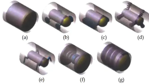
1-1 Different design configurations of in-pipe robots. (a) Pig type. (b) Wheel type. (c) Caterpillar type. (d) Wall-press type. (e) Walking type. (f) Inchworm type. (g) Screw type. [3] . . . . 16 1-2 Two main categories for maneuvering mechanisms: differenential drive

joint type, as shown in (c) and (d), and articulated active joint type,

as shown in (a) and (b). [3] . . . . 17

2-1 Image of the deformed (bent) and undeformed rectangular cuboid. [13] 26 2-2 Schematic simplifying the bending profile of an individual joint as it

maneuvers through a T-junction. The dimensions appearing on the figure are in mm. The joint is outlined in red, while the pipeline is sketched in black. The image is not drawn to scale. . . . . 27 2-3 Schematic of the spring-inertia-dashpot model considered. From the

experiments conducted, values for the physcial parameters, I, B, and K, will be deduced, once values for C, we, and A are determined. . . . 28

3-1 Schematics showing the overall structure of the snake-like robot with the propulsion system at the back and the wall-press friction control mechanism for speed control (pointing radially outward from the outer surface of the robot). (a) presents the highly maneuverablle structure of the robot. (b) presents the robot manuevering through a T-junction along the in-service pipeline. A single joint is outlined in the red box. The development of such joint is the focus of the paper. . . . . 30

3-2 The robot, modeled as a cylinder with length h and width (diameter) w in a junction. Two cases appear, in contrast to (b), in (a) the ends of the robot are located within the straight parts of the junction. [2] . 31

3-3 Geometric constraints on the robot's size. In order to avoid jamming, the robot's length, h, and diameter, w, must lie under the the line, depending whether in case (a) or (b) described in Figure 3-2. . . . . . 32

3-4 Angular acceleration, a as a function of the velocity of the module,

Vm. Two cases appear; max a refers to the angular acceleration once

the joint end has deflected an angle of 7r/2; average a represents the average angular acceleration over the time of deflection of an angle of

7r/2. . . . . 33

3-5 Measurement of the drag force acting on the stagnant robot due to varrying fluid flow speeds-worst case scenario. . . . . 34

3-6 Schematic assisting in showing how the torque requirement due to drag effects was simplified and approximated. w is the diameter of the robot, which was approximated as 65 mm. When the robot approaches a junc-tion, the wall-press "elbows" of the robot retract to allow for sufficent room for maneuvering, as appears in the figure. Lengths appearing in the figure are in mm and are not drawn to scale . . . . . 35

3-7 3-D View at an angle of a single rigid compartment that houses the servo-motor and its supporting structures, from which the tendon-s/wire are extended through the the two holes of 3 mm appearing in the figure. Lengths displayed on the figure are in mm. . . . . 36

3-8 Cross-sectional top view of the joint displaying its internal compo-nents. The servo horn that is mounted on top of the servo motor appears in gold. The servo motor appears in blue. The pulley appears in grey. The tendons/wires that are mounted onto the servo horn and extended through the pulleys to the outside of the compartment, through the rubber material, to the other rigid compartment, appear in red. The tendons/wires that appear in green are extended from the other rigid compartment and mounted to this compartment at the locations shown. The other compartment is 90 degrees out of phase (with respect to its roll orientation) and is positioned at the other end of the flexible rubber (not shown on figure). Lengths displayed on the figure are in m m . . . . 37

3-9 The rigid compartments are designed such that once the motor is mounted, the servo horn is attached on top of it, the tendons are put in place as can be seen in detail in Figure 3-8, the compartment is closed. The two parts appearing in the figure (top and bottom) are then screwed to each other and sealed to assure no water entrance into the compartment, therefore damaging the equipment in the inside. . . 38

3-10 Front view of the rigid compartments of the joint. Left: image as the joint would appear from the outside. The holes (of 3 mm diameter) from which the wires/cables will exit the joint appear. Right: image of a front view cross section displaying the interior of the compartment shown to the left. The servo horn appears in gold, the servo motor appears in blue, and the pulleys appear in grey. Lengths displayed on the figure are in mm . . . . 39

4-1 Display of the functional joint as it bends. Its tip goes from an angular displacement of zero at (a) to 7r/2 at (h). . . . . 46

4-2 Different displays of a single joint resting on the table. The black part and the green part at each end of the joint are the rigid compartments. The white part is the flexible component of the joint, which is made from rubber. The image to the right shows the definition of angle 0. . 47 4-3 (a), (b), (c), and (d) present snapshots of the impulse response of the

system, measured as the vertical displacement of the free end of the joint, while the other end is mounted in place. The images present the progression of the video analysis conducted, which starts at configura-tion (a) and ends at (d). . . . . 47 4-4 Display of the experimental set-up for the step response experiment.

(a) displays the elavation of the red point marked on the free end of the joint end relative to a known reference point, prior to the step force input. (b) presents the elavation of the red point marked after the joint reached a final steady state configuration while subjected to the force step input (from the mass hanging). . . . . 48 4-5 The impulse response of the system, measured as the vertical

displace-ment, Y(t), of the end of the joint (in cm) from the horizontal straight orientation of the joint as a function of time (in s). The response of the system displays a standard underdamped system response with O<Q<1. 48

List of Tables

4.1 displays values of the system parameters obtained from the analysis of the impulse response of the system. As appears below, values for

C

system's transfer function. Particularly, values for effective inertia, I, effective stiffness, K, effective damping, B, and the compliance of the joint (equal to the static gain, A), are displayed below. . . . . 45

Chapter 1

Introduction

1.1

Motivation for In-Pipe Leak Detection

Leaks in water distribution pipelines lead to significant losses of resources; the

elim-ination of such losses is crucial for efficient water resource management. Pipeline

distribution networks have been widely used as means of transport of different fluids,

including water. Due to corrosion, bad workmanship, cracks or normal wear and

dam-age, water pipeline distribution networks can be subject to significant loss of energy

and resources. Vickers reports water losses in USA municipalities to range from 15

to 25% [18]. The Canadian Water Research Institute reports that on average 20% of

the treated water is wasted due to losses during distribution [1]. A study on leakage

assessment in Riyadh, Saudi Arabia, shows the average leak percentage of the ten

studied areas to rise up to 30% [1]. As evident by such reports, losses through leaks

represent a significant portion of the water supply. Such losses make the identification

and elimination of leaks crucial for efficient water resource management.

In-pipe robots equipped with appropriate sensing capabilities have high potential

for accurate, efficient, and inexpensive leak detection. Such robots have been widely

explored for leak detection in water distribution systems. They can be deployed

for inspection through fire hydrant stations and left to autonomously inspect the

distribution pipeline network without the need to shut-off the system or the need for

operator intervention. Due to the advantage of being able to go as close as possible

to the leak source, they are best suited for potential highly accurate and reliable leak

detection.

1.2

Types of In-Pipe Inspection Robots

In-pipe inspection robots come in different design configurations with diverse

mo-tion attributes. Their differences can be with respect to their movement patterns

while in motion, ability to handle complex pipeline geometry, and type of joints

em-ployed for robotic maneuvering. According to

[3],

they can be classified according

to their movement pattern into one or more of the seven main categories (types), as

shown in Figure 1-1: pig, wheel, wall-press, walking, caterpillar, inchworm, and screw

types. The robots developed up to date can generally travel across simple horizontal

pipelines. However, only a fraction of them can handle more complex pipeline

con-figurations (vertical pipes, L-junctions, Y-junctions, T-junctions, etc.)

[3].

Due to

the complexity of the existing water pipeline distribution systems, it is essential for

in-pipe robots to be able to handle such pipeline geometries, therefore making the

passive approach inadequate.

(a)

(b)

(c)

(d)

(e)

(f)

(g)

Figure 1-1: Different design configurations of in-pipe robots. (a) Pig type. (b) Wheel

type. (c) Caterpillar type. (d) Wall-press type. (e) Walking type. (f) Inchworm type.

(g) Screw type. [3]

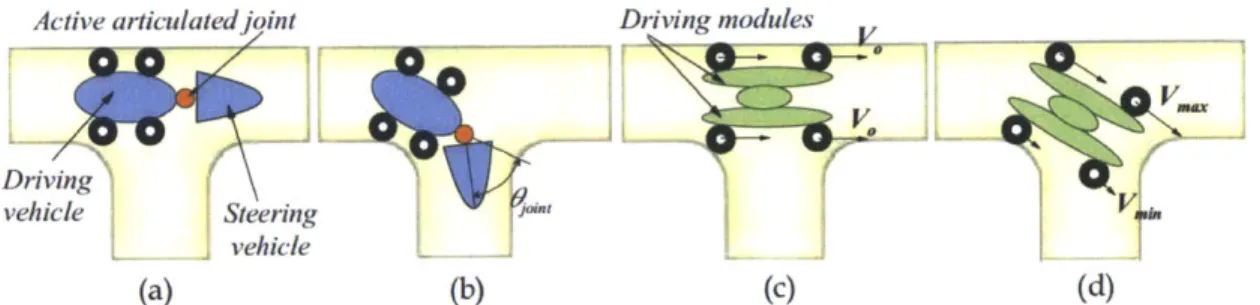
with maneuvering mechanisms, which can be largely divided to two main categories.

First, differential-drive; through the velocity differential of the driving wheels at

op-posite ends of the robot, the robot is able to maneuver in different directions, as

shown in Figure 1-2 (d). Second, articulated active joints; in their movement, robots

that fall under this category resemble means of locomotion of worms, snakes, elephant

trunks, etc. According to

[6],

robots that fall under the latter category are termed,

articulated mobile robots. Such robots come in different forms: discrete, serpentine,

and continuum

[6].

Discrete mobile robots are generally assembled from a series of

modules that are linked via joints. Serpentine robots, while similar to discrete mobile

robots in the use of joints that connect different modules and allow for articulated

maneuvering ability, they generally combine many short rigid links (or joints). Such

feature allows these robots to have higher mobility, through their ability to deform

the robot into smooth shapes, similar to snakes, eels, and worms [6]. Finally,

contin-uum robots, as described by [6], are not composed of rigid links or rotational joints.

Via elastic deformation, these robots are able to bend continuously along their length

and move in locomotive mechanisms similar to tentacles.

Active articulated joint Driving modules

Driving

vehicle Steering

L_ vehicle

(a)

(b)

(c)

(d)

Figure 1-2: Two main categories for maneuvering mechanisms: differenential drive

joint type, as shown in (c) and (d), and articulated active joint type, as shown in (a)

and (b). [3]

Among the different options available for the robot's pattern of movement, the

wall-press mechanism was pursued in the work presented, as shown in Figure 3-1.

The choice of this type of in-pipe robot conveniently allows for the attachment of

different leak detection sensors around the perimeter of the robot, the attachment

of a propulsion system at the front or end of the robot, and the use of the

wall-press mechanism as means of speed control in the pipe through friction control

[1].

Friction control, in part, is achieved through varying the normal force that the robotic

"elbows", as shown in Figure 3-1, apply on the pipe's interior surface.

1.3

Functional Requirements

This robot is developed to satisfy several functional requirements. First, autonomy

and wireless operation; the system is capable of completing full inspection of a

par-ticular portion of a water distribution network autonomously and wirelessly. The

only constraints are limits with regards to battery energy capacity and

communica-tion range. Second, leak sensing sensitivity; the system is able to detect small leaks

in plastic (PVC) pipes, which are among the most difficult pipes for leak detection,

given the damping of sound and vibrations in the pipe itself [1]. Third, working

conditions; in order to be cost effective to the water distribution and management

authority, the system is designed to operate in the water distribution network while

in-service. In such setting, the flow conditions are expected to be as follows: a line

pressure of 1 to 5 bars and a flow speed of 0.5 to 2 m/s. Fourth, communication; the

system is able to (a) communicate with stations above ground and pinpoint potential

leaks in the water network, (b) store information and transmit the information/data

collected upon completion of the pipeline inspection cycle to allow for data analysis.

Fifth, maneuverability; the robot should be highly maneuverable to avoid jamming

and to handle the different junction types encountered while it inspects the pipeline

network. Sixth, localization; driven by a need for accurate leak position estimation

and the retrieval of the robot upon inspection completion, the system is developed

with the capability of localizing itself within the water distribution network [1].

1.4

Maneuvering Mechanisms

The numerous maneuvering mechanisms explored in the literature involve pneumatic,

shape memory alloy (SMA), piezoelectric, tendon-driven, universal joint-based, and

traditional gear-based actuators. These maneuvering mechanisms enable in-pipe robots to handle different junctions present in complex pipeline networks. The Dou-ble Active Universal Joint (DAUJ) is among the universal joint-based actuators men-tioned above. The DAUJ has two degrees of freedom and has been used to maneuver the gas-pipeline inspection robot described in the work of [14]. The gear-based actu-ator/transmission system used to enable the Explorer, an in-pipe inspection robot, to maneuver employs a mechanism that occurs through a roll-pitch joint arrangement

[15]. Two roll joints are positioned at the inside edge of every drive module and an ac-tive pitch-joint is placed at every dually interconnected module. The roll-joints allow the entirety of the robotic train to rotate about its longitudinal axis [15]. The active pitch-joint enables successive joints to be rotated in a plane set by the orientation of the roll-actuators [15]. A cylindrical piezoelectric actuator allows maneuvering in 3 dimensions. Such actuators have been reported in the literature, [7] and [8]. However, the performance of piezoelectric actuators falls short in the application considered; while highly controllable and precise, piezoelectric actuators are only capable of rela-tively small deformation/bending displacements. Maneuvering of in-pipe robots could also be done through the employment of temperature controlled shape memory al-loys for the joints, as described in [19] and [17]. In [19] and [17], motion actuation and maneuvering is achieved through the utilization of the phase transition of shape memory alloys (SMA). Bending of such structure/joint is achieved by current con-trolled localized heating. Once heating is stopped, the structure returns to its default shape, given its SMA characteristics [19]. The use of pneumatic-based actuators for joints could be found in [5]. The actuator is made of a rubber tube wrapped with a nylon sleeve and two tip supports as presented in the work of [5]. The rubber tube stretches and shrinks based on the pressure of the hydrogen gas it encloses, which is supplied through the heating of a hydrogen storage alloy. The fabric nylon sleeve, in turn, converts the deformation of the rubber tube into elongation along the length of the pressurized tube. The pressure control that is used to drive the actuators is realized by the electrical temperature control. The bending capability of the joint is accomplished through the harmonic stretching and shrinking on each of the four

driving actuators attached along the surface area along the length of the cylinder modeled rubber tube [5]. Other joints explored in the literature could be found in

[16], [10], [4].

1.5

Scope of Work

This work is focused on the design, analysis, evaluation, and prototyping of active tendon-driven flexible robotic joints that connect the sub-modules of a snake-like robotic platform. Among the different types of articulated mobile robots described above, a combination of the continuum and serpentine robots is adopted. Such com-bination offers high mobility due to the robot's ability to deform into smooth shapes and conform to the complex pipeline environment. The justification for the selection of such joint among the several options mentioned will be clarified in a following section. The joint developed and experimented upon enables the robot to handle dif-ferent junction types (elbow, T, Y, and L) in active water distribution plastic pipelines of 100 mm diameter. The robot is expected to be autonomous, whereby each joint is controlled as the robot approaches a junction in order to achieve a particular turning trajectory. As such, the determination of the mechanical properties of the robotic joint is essential. It gives insight into how the joint may be controlled and provides grounds for simulation of the robot's motion in the pipeline network.

1.6

Joint Functional Requirements

The main focus of the paper is the development of a novel flexible tendon driven joint that connects sub-modules of an in-pipe snake-like robot. The joint enables the robot to maneuver in complex pipeline geometry. The joint is developed to satisfy the following functional requirements:

* Ability to handle complex pipeline geometry: the joint is expected to allow for the

robot to handle straight pipelines and different junctions (elbow, T, Y, and L) in the pipeline network at different module speeds (0.5-1 m/s), without being stuck and

with minimal collision with the inner pipe walls.

a Water sealing characteristics: the joint is ideally well-sealed to prevent water leakage

into the robot, which could damage its different electrical/mechatronic components.

* Size: Water pipes of 100 mm internal diameter are of interest in the present work,

given their wide use in most water distribution networks. The internal diameter of the pipe imposes a geometric constraint on the size of the robot. Therefore, it is essential for the joint developed to not exceed a diameter of roughly 65 mm, in order to allow for sufficient space for the attachment of the friction based speed control mechanism discussed in detail in [1]. In addition, with respect to length and shape of the joint, it is important for the robot not to jam in the pipe. In the case of a robot modeled as a rigid cylinder, the constraints on the length and diameter are outlined in Chapter 3. In short, the robot must be developed with a design that is highly maneuverable, adaptable to the pipeline environment, and preferably non rigid in order to avoid jamming.

e Robustness: the joint developed should be able to function reliably in varying pipe

fluid flow conditions and should be usable for more than a handful of inspection runs without the need for repair.

e Controllability and precision: the joint must be controllable with high enough pre-cision in order to achieve smooth and timely maneuvering trajectories once the robot approaches the different junctions.

e Minimal flow invasiveness: the robot should be minimally invasive to the water flow in the pipe in order to not disturb the signal captured (acoustic for example) from the leak source along the pipe.

1.7

Justification for Joint Selection

As previously mentioned, active tendon-driven flexible joints were employed in this work to enable the robotic platform to maneuver. Such joints were selected among the many maneuvering mechanisms mentioned earlier due to the match between their performance and the joint functional requirements outlined above. Given that in the

design pursued, the joint is made from a rubber material with the tendons embedded along its length, such joint design naturally offers water sealing characteristics. With respect to size, the joint type selected allows the robot to be highly maneuverable, due to its ability to bend in many forms and to its adaptability to the pipeline environment. As such, there aren't any concerns with jamming. With respect to robustness, while this is the down side to the use of such joint in comparison to the rigid joints, for example, it is believed that the joint offers sufficient robustness that would allow the robot to function reliably. With respect to controllability and precision, the tendon driven approach is highly controllable and offers high precision, as evident in the use of such joints in surgical manipulators. Finally, with the tendon-driven joint design, the robot is developed to be minimally invasive to the flow of water in the pipe. This is achieved by the smooth continuous deflection profile of the robot, as well as the uniform diameter profile of the robot. As such, the signal from leaks could be clearer and have relatively less noise generated from the flow of the robot in the pipe.

1.8

Organization of Thesis

The document is composed of five chapters. Chapter 2 deals with the analysis em-ployed to design the tendon-driven robotic joint. Chapter 3 presents the design and method of prototyping of individual joints. Chapter 4 presents the testing of the functionality of the robot, as well as the experimental set-up, data collection, and data analysis used to obtain the mechanical properties of the joint. Chapter 5 covers the conclusions and recommendations.

Chapter 2

Analysis

This section deals with the analysis and design of the proposed robotic joint. The analysis presented in section 2.1 allows for the estimation of the torque required to maneuver the robotic platform through a junction in an in-service pipeline network. Section 2.2 presents the analysis conducted to estimate the mechanical properties of the joint through dynamic modeling and system identification.

2.1

Maneuvering Analysis

The snake-like robot is expected to be able to maneuver (or steer) through junctions in water distribution plastic pipelines. To achieve this task, the joint is expected to overcome the inertial effects due to the angular acceleration as the joint maneuvers, drag effects due to the robot's interaction with the water in the pipe, stiffness effects (since the flexible joint as an effective stiffness that will resist bending), and damping effects. In order to develop the joint, it is necessary to estimate the torque required to allow the flexible tendon-driven robot to maneuver in a pipeline geometry. Given a water flow speed between 0.5-2.0 m/s in pipes of 100 mm diameter, the fluid flow will be well into the turbulent regime, as Re>2300. The total torque required to overcome such effects described above, T, can be found using the following expression:

whereby TD is the torque requirement due to drag as the joint maneuvers in a pipe

with active water flow; T, is the torque requirement due to inertial effects, which arise from the angular acceleration during maneuvering; TB is the torque requirement due to bending/stiffness effects as the joint is expected to resist bending. The torque required to overcome damping effects does not appear in the equation above, given that it is expected to be negligible in comparison to the other effects.

There is no theoretical formulation describing the torque experienced by a robot (modeled/approximated as a cylinder) as it moves along an arbitrary curved path (in order to maneuver at a junction along the pipeline network). That is because both the the cross sectional area, Ac., and the drag coefficient, CD, described in equation (2.2) vary along the turning trajectory. As a result, the torque required to overcome drag effects, TD, is precisely estimated via experimentation or Computational Fluid

Dynamics (CFD).

Given that in this work, TD (and T accordingly) is estimated in order to size

the actuator needed to enable to robot/joint to maneuver, a less rigorous approach was taken, as can be seen in Chapter 3. Using this approach, TD can be estimated

according to the following expression:

TD = 12pCDAcsAV 2, (2.2)

whereby pw is the density of water (about 1000 kg/m 3), Ac, is the cross sectional

area of the robot (in M2), CD is the drag coefficient, and AV is the relative velocity

of the water with respect to the robot (in m/s).

The torque requirement due to inertial effects, TI, could be calculated according to the following expression:

T, = Ia, (2.3)

whereby I is the moment of inertia (in kg _ M2

), and a is the angular acceleration (in

rad/s2_{), which is equal to the second derivative with respect to time of the angle, 0,}

could be approximated using the following expression:

aavg Aw/At, (2.4)

whereby At is the change over time (in s), and Aw is the change in angular velocity (in rad/s); angular velocity, w, is the rate of change with respect to time of the angle

0, defined in Figure 4-2.

Another expression for angular acceleration a, could be obtained by the integra-tion of equaintegra-tion (2.4) with the assumpintegra-tion that a is constant:

a 2(AO - wit)

t2

whereby wi is the initial angular acceleration (in rad/s), AO is the change in angular displacement (in rad), and t is time (in s).

Finally, the torque requirement due to bending effects, TB, is discussed. Given that the joint is made out of rubber, constitutive relations of hyper-elastic solid mechanics are used to calculate the moment needed for flexure/bending of the joint. The deflection considered here, as shown in Figure 2-2, is in the order of magnitude of the diameter of the cylindrically modeled joint. So, a method for handling large elastic deformation of homogenous isotropic materials must be employed. The moment is approximated by assuming the bending of a rubber rectangular cuboid in cartesian coordinates. As shown in Figure 2-1, the rectangular cuboid has the following faces: x=ai and x=a2 whereby a1> a2; y=±b; and z=±c. According to [9], [11],[13], the

expression for the bending moment, TB, is as follows:

TB

=

8c(al

(2.6)

3

whereby C1 and C2 are physical constants [13]. The model assumed that the material is isotropic, volume change and hysteresis are negligible, and the shear is propor-tional to traction by uniform contraction or dilatation only [11]. C1 and C2 may be

calculated based on the following expressions:

C1

=

(G + H)/4

(2.7)

and

C2= (G

- H)/4

whereby G is the modulus of rigidity (material property G=0.0003 GPa for Rubber) and H is the modulus characterizing asymmetry of reciprocal deformations, another physical property of the material. c may be calculated according to the following expression:

E_=[1- _=[I

_(a-

r

(2.9)

a 2

a,

whereby r1 and r2 are what surfaces x=al and x=a2 turn to when the rectangular cuboid is subject to bending/flexure. In particular, surfaces of the undeformed body x=ai and x=a2 become parts of the curved cylinders of radii r1 and r2 respectively,

as can be seen in Figure 2-1 [13].

t an dr

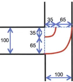
J 65

T

35

100

65

Figure 2-2: Schematic simplifying the bending profile of an individual joint as it

maneuvers through a T-junction. The dimensions appearing on the figure are in mm.

The joint is outlined in red, while the pipeline is sketched in black. The image is not

drawn to scale.

2.2

Dynamic Modeling and System Identification

The snake-like robot is designed to handle different junctions in water distribution

pipelines. So, the joint is expected to overcome effects that are associated with drag,

inertia, bending/stiffness, and damping, as expressed earlier. As such, the system is

anticipated to act as a second order system. For simplicity, the analysis performed

on the joint was not done based on experimentation in an active water pipeline.

Therefore, the model presented does not account for the drag effects that would

be present in the real application of the robotic system (while still accounting for

bending/stiffness effects as well as inertial effects).

The transfer function of a second order system can be determined once three

parameters are identified. These parameters are damping ratio, C, natural frequency

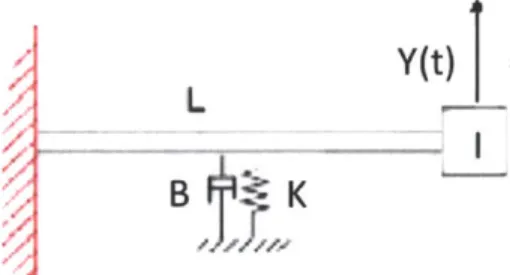
of oscillation, Wn, and static gain, A. Figure 2-3 presents a schematic of the model

considered. As shown in equations (A.5) through (A.7), C,

and A are written

in terms of the physical parameters, I, B, and K. These are the effective inertia,

damping, and stiffness, respectively.

Y(t)

L

-B

K

Figure 2-3: Schematic of the spring-inertia-dashpot model considered. From the

ex-periments conducted, values for the physcial parameters, I, B, and K, will be deduced,

once values for (, w, and A are determined.

2.3

Summary

This chapter introduced the analysis and design of the individual joints. The

esti-mation of the torque required to maneuver the robotic platform through a junction

along the in-service pipeline network is shown. Also, the analysis conducted on the

experimental data, as described in Chapter 4, was introduced. This allowed for the

estimation of the mechanical properties of the joint through dynamic modeling and

system identification.

Chapter 3

Design and Prototyping

This chapter deals with the design and prototyping of individual joints. Section

3.1 goes over the general design of the snake-like robotic platform. The shape and

size constraints imposed on the robot by the pipeline geometry are discussed with

reference to maneuverability of the robot. Section 3.2 discusses the actuator torque

requirement specification. Sections 3.3 and 3.4 present the design and prototyping of

the joints.

3.1

Design of In-Pipe Robot

A snake shaped robot developed from the assembly of multiple flexible tendon-driven

joints was selected for the overall design. There are two main reasons for such choice of

overall shape for the robotic platform. First, it has a high length to diameter ratio. As

a result, a snake-shaped robot provides an efficient design. It allows for sufficient space

to place the different robotic sub-systems (battery packs, data processing, sensing

module, etc.) onto the robotic platform, while satisfying the geometric constraints

that the pipe geometry imposes on the shape of robot and its dimensions (length

and diameter). Second, a snake-like robot, has high degree of maneuverability and

adaptability to the pipeline environment. A schematic of the overall shape of the

robot appears in Figure 3-1. You may note the propulsion system at the back of the

robot. You may also note the wall-press friction-control mechanism for speed control

pointing radially outward from the outer surface of the robot, which is described

thoroughly in the work of [1].

The white parts that appear in the schematic are

the flexible tendon-driven robotic joints that enable to the robot to maneuver in 3-D

regardless of its roll orientation. These joints are the focus of the paper; the design

of these joints will be thoroughly covered in the following sections. The grey parts

of the robots that appear in Figure 3-1 are the solid components of the robot, which

carry the robot's different modules for data processing, power (battery packs), sensing

devices, visual inspection device, communications, control, and data storage, etc.

(a)

Propulsion Rigid Rubber

Psysem compartments

(b)

Figure 3-1: Schematics showing the overall structure of the snake-like robot with the

propulsion system at the back and the wall-press friction control mechanism for speed

control (pointing radially outward from the outer surface of the robot). (a) presents

the highly maneuverablle structure of the robot. (b) presents the robot manuevering

through a T-junction along the in-service pipeline. A single joint is outlined in the

red box. The development of such joint is the focus of the paper.

3.1.1

Maneuverability and Size Limitations

The internal diameter of the pipeline network and the geometry of the different

junc-tions along the pipeline place geometric constraints on the shape and size of robot.

To provide an estimate of the geometric limits on the dimensions of the robot flowing

through an elbow junction, the robot is modeled as a cylinder with diameter, w, and

length, h.

450

~

D

R

(a) (b)

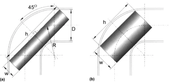
Figure 3-2: The robot, modeled as a cylinder with length h and width (diameter) w

in a junction. Two cases appear, in contrast to (b), in (a) the ends of the robot are

located within the straight parts of the junction.

[2]

For case (a), according to Choi et. al., the maximum length of the module, h,

could be found using the following expression:

h

2V'2[D/2 + R

-

(R

-

D/2 + w)cos45

],

(3.1)

whereby R is the radius of curvature of the junction, taken as equal to the diameter

of the pipe in this case, as appears in Figure 3-2 (a), and D is the diameter of the

pipe.

For case (b), the maximum length of the module, h, could be found using the

following expression

[2]:

h = 2/(D/2 +

R)2

(R

-

D/2+ w)2.

(3.2)

In order to satisfy the geometric constraints described in equations (3.1) and (3.2),

the length of the module, h, and the diameter of the module selected, w, must be

under the line appearing in Figure 3-3, depending on the case satisfied (a or b, as

appearing in Figure 3-2).

For the specific prototype built and presented in this paper, the internal diameter

of the pipe network was 100 mm (D=100 mm) and the diameter of the module was

about 65 mm (w=65 mm). For this value of w, the maximum length permissible

to avoid the module from getting stuck is approximately 195 mm, as can be seen in

Figure 3-3.

-Case

(a)

240

-Case

(b)

EP

220

S200

-160

-14%

50

60

70

80

Diameter of Module (mm)

Figure 3-3: Geometric constraints on the robot's size. In order to avoid jamming, the

robot's length, h, and diameter, w, must lie under the the line, depending whether in

case (a) or (b) described in Figure 3-2.

3.2

Actuator Torque Specification

The analysis section investigated the sizing of the actuator (servo-motor). Equations

(2.1) through (2.9) were used to estimate the torque required to maneuver a single

robot joint. The leading joint, outlined with navy dashed lines in Figure 3-1 (b), is

referred to. The torque required to maneuver the joint is due to the need to overcome

inertial, bending/stiffness, and drag effects.

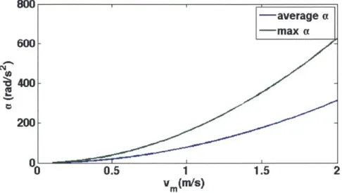
The torque required to overcome inertial effects is primarily dependent on the

speed of the robot in the pipe as it approaches a junction. The effect of the speed

of the robot as it approaches a junction on angular acceleration (which relates to T,

in the pipe, moving at the speed of the fluid flow. This assumption holds unless the

robot is required to speed up or slow down. Slowing down would be desirable as the

robot approaches a junction, or when it senses the presence of a leak. In that case,

the robot will use it's wall-press friction controlling mechanism in order to decrease

its speed. According to equation (2.2) and Figure 3-5, it can be seen that the drag

force is proportional to AV

, as expected. In order to develop an energy efficient

robot, it is desirable to reduce the torque requirement as much as possible, while still

being able to maneuver the robot.

800

-average

a

-max

a

600-

-

~400-

200-0

0.5

1

1.5

2

Figure 3-4: Angular acceleration, a as a function of the velocity of the module,

Two cases appear; max a refers to the angular acceleration once the joint end has

deflected an angle of 7r/2; average a represents the average angular acceleration over

the time of deflection of an angle of 7r/2.

The torque required to overcome drag effects is primarily dependent on the

dif-ference in speed of the water flowing in the pipe and the robot. Given that a rough

approximation of the torque requirement is sought in this analysis, we may simply

calculate the worst case scenario (maximal FD), whereby the robot is completely

stagnant, and the cross sectional area that appears in equation (2.2) (needed for the

calculation of the drag force) is a rectangular shape with dimensions 35 mm by 65

mm (area obtained by orange cross-sectional area pointing 65 mm into the page, as

can be seen in Figure 3-6). In such case, the difference in velocity of the water and

that of the robot, AV, is equal to the speed of the water. The dependence of

on

AV for such case is shown

inertial effects, in order to

reduce the drag force,

robot.

3I

in Figure 3-5. Similarly to the torque required to overcome

obtain an energy efficient robot, there is an incentive to

as much as possible, while still being able to maneuver the

3

2-

1m

0.5

0

0.5

1

A

V(m/s)

1.5

2

Figure 3-5: Measurement of the drag force acting

varrying fluid flow speeds-worst case scenario.

on the stagnant robot due to

By inspection of Figures 2-1 and 2-2, it may be seen that upon approximating the

red lines appearing in Figure 2-2 as circular arcs, r

=100 mm and r

=35 mm. a,

and a

are to be calculated depending on the undeformed shape of the beam modeled

rubber joint. G is approximated as 0.0003 GPa; it is considered an approximation,

given that the properties of the rubber material are adjustable based on the method

of preparation, which will be described in detail in Chapter 4. A more accurate

measure for G obtained for the specific method of preparation of the rubber material

could be done via experimentation; in particular, by taking the slope of the shear

stress-shear strain graph, which is equal to G. As for H, that value is to be estimated

via experimentation. For an incompressible Neo-Hookean material, whereby perfect

elasticity is assumed,

is equal to zero (C2=0) [13]. c is calculated depending on the

values assigned to a, and a

. c=32.5 mm, assuming the cylinder with a diameter of

65 mm is approximated as a rectangular cuboid with a thickness bounded by places

z=±32.5 mm.

35

100

Figure 3-6: Schematic assisting in showing how the torque requirement due to drag

effects was simplified and approximated. w is the diameter of the robot, which was

approximated as 65 mm. When the robot approaches a junction, the wall-press

"elbows" of the robot retract to allow for sufficent room for maneuvering, as appears

in the figure. Lengths appearing in the figure are in mm and are not drawn to scale.

3.3

Joint Design

Individual joints referred to in this section are the the sub-parts of the robot that

allow it to maneuver in 3-D by the use of two degrees of freedom (DOF) per joint.

An individual joint is outlined in the red box appearing in Figure 3-1. It is composed

of two rigid compartments that are made from plastic and are fabricated using 3-D

printing technology with a flexible part in between, that is made from rubber. Each

of the rigid components, as appears in Figures 3-7, 3-8, and 3-7, houses a servo-motor

(appearing as a blue box in Figure 3-8), along with its support structures

(servo-horn-appearing in gold-, two pulleys, and a wire-(servo-horn-appearing in red-that extends from the

each compartment through the flexible robot as a tendon, to the other compartment

where the wire is mounted). Each of the compartments is responsible for maneuvering

the flexible part up to ±90 degrees along a single degree of freedom. By placing the

two rigid compartments at 90 degrees out of phase in their roll orientation, the joint

is capable of maneuvering in 3-D by the use of either or both DOF, depending on its

particular roll orientation at that time.

Figure 3-7: 3-D View at an angle of a single rigid compartment that houses the

servo-motor and its supporting structures, from which the tendons/wire are extended

through the the two holes of 3 mm appearing in the figure. Lengths displayed on the

figure are in mm.

3.4

Prototyping

The rigid compartments are designed such that the motor along with the servo horn

and the wire attached to it are mounted onto the lower part, which appears in Figure

Figure 3-8: Cross-sectional top view of the joint displaying its internal components.

The servo horn that is mounted on top of the servo motor appears in gold. The

servo motor appears in blue. The pulley appears in grey. The tendons/wires that are

mounted onto the servo horn and extended through the pulleys to the outside of the

compartment, through the rubber material, to the other rigid compartment, appear

in red. The tendons/wires that appear in green are extended from the other rigid

compartment and mounted to this compartment at the locations shown. The other

compartment is 90 degrees out of phase (with respect to its roll orientation) and is

positioned at the other end of the flexible rubber (not shown on figure). Lengths

displayed on the figure are in mm.

3-9 (down), and the wires are arranged such that they would exit the compartments

through two specified holes. Once two solid compartments are assembled and are

facing each other, but out of phase by 90 degrees along the roll axis, they are inserted

into a fabricated mold, and placed at a specified distance. The mold is closed and the

flexible material in the form of a highly dense liquid is injected into the mold and left

to "solidify". Once the flexible part solidifies, the motors are powered by a battery

and controlled via remote control.

The compartment, the servo-horn, and the two pulleys were fabricated using 3-D

printing technology. The motor selected is manufactured by HiTech and is called

HS-Figure 3-9: The rigid compartments are designed such that once the motor is

mounted, the servo horn is attached on top of it, the tendons are put in place as

can be seen in detail in Figure 3-8, the compartment is closed. The two parts

ap-pearing in the figure (top and bottom) are then screwed to each other and sealed to

assure no water entrance into the compartment, therefore damaging the equipment

in the inside.

7954SH Servo. It is modifiable for 360 deg. rotation, and suitable dimension wise (40

x 20 x 37mm). It is capable of producing a stall torque of 402 oz.in (2.84 N.m) and

a no load speed of 0.12 sec/60 deg (8.7 rad/s) at 7.4V. The flexible material is

Plat-inum Cure Silicone Rubber, under the brand name, "Ecoflex Supersoft Silicone 0010".

Figure 3-10: Front view of the rigid compartments of the joint. Left: image as the

joint would appear from the outside. The holes (of 3 mm diameter) from which the

wires/cables will exit the joint appear. Right: image of a front view cross section

displaying the interior of the compartment shown to the left. The servo horn appears

in gold, the servo motor appears in blue, and the pulleys appear in grey. Lengths

displayed on the figure are in mm.

3.5

Summary

Chapter 3 discussed the design of the overall in-pipe robot and the individual joints

that enable it to maneuver through complex pipeline geometries. Maneuverability

and size limitations imposed on the design of the in-pipe robot by the pipeline

ge-ometry were specified. In addition, servo-motor torque estimation needed for sizing

the actuators that enable individual joints to maneuver was analyzed. Lastly, the

procedure for prototyping individual joints was discussed.

Chapter 4

Experimentation and Analysis

The first part of this chapter, sections 4.1 and 4.2, discusses the experiments con-ducted. The first experiment was conducted to test the functionality of the joint designed and prototyped (4.1). The second and third experiments were conducted to generate the data necessary for analysis. The second part of this chapter, sections 4.3 and 4.4, goes over the analysis of the joint's mechanical properties via dynamic mod-eling and system identification. These techniques were used for the determination of the system parameters and mechanical properties.

4.1

Experimentation on Functionality of Robotic

Joint

To assure correct function of the robot, the robotic joint was tested for the case of in-plane maneuvering. For experimentation purposes, the servo motors were controlled using a micro-controller programmed to communicate with a remote control in the hands of the operator. One end of the joint was held in place while the other was left free. Snapshots taken from a video showing the joint's end maneuvering through an angular displacement of 7r/2 are presented in Figure 4-1.

4.2

Experimentation for Data Analysis

In this section, the experimental set-up, data collection, and data analysis using system identification techniques will be presented. This work is expected to provide grounds for simulation development for the modeling and control of the robotic joint as it inspects the in-service pipeline. The following sections are concerned with the system identification of the robotic joint itself, in the absence of the effects associated with the joint's interaction with the water, as it maneuvers in the pipe.

Two experiments were conducted to determine the mechanical properties of the joint. To obtain values for the damping ratio,

C,

4.2.1

Impulse Response Experiment

To obtain the data for the impulse response experiment, the joint was first set-up on a table, in a horizontal orientation, with one end of the joint held, while the second end was free to move. Once the free end of the joint was oscillating due to the impulse applied, a high-speed camera recorded its movement. The video was analyzed using Logger Pro and the plot for the displacement of the end of the joint as a function of time, Y(t), was generated. System identification techniques were carried out to obtain values for

C

Set-Up

A preliminary test was needed to understand the joint better, and thus a dry test was performed in place of a wet test. The experiment was done while the joint was lying horizontally on a table. The purpose behind this horizontal orientation and set up was to eliminate the effects of gravity on the periodic motion of the joint. The

basic experimental set up may be viewed in Figure 4-3.

One end of the joint was held still, while the other end of the joint was left untouched. The untouched end of the joint was marked with a sticker to assist in visualizing the displacement of the end of the joint in the video analysis. A high-speed camera, namely, Samsung TL350, was affixed at a particular height in order to capture the motion of the end of the joint as oscillated. A speed of 1000 frames per second was assigned to the camera.

Procedure and Analysis

Once the end of the joint was oscillating due the impulse input, the camera started recording the motion of the end of the joint until the displacement of the end of the joint reached a steady state value at 0 cm. This set-up may be understood by observing Figure 4-3.

Video analysis was carried out using Logger Pro. Once the data was gathered and the plot of displacement of the end of the joint, Y(t), was generated, the data was analyzed. The response of the system displayed characteristics of an underdamped second-order system. From the impulse response, C could be determined by curve fitting of the decaying envelope of the response. w, was determined through observing the frequency of oscillation (or through observing the period of oscillation). The response of the system may be viewed in Figure 4-5 below.

4.2.2

Step Response Experiment

The static step response experiment was conducted in order to quantify the value of the static gain, A. It's value could not be obtained from the analysis of the impulse response function, given that the impulse was of unknown magnitude. To obtain the data for the static step response experiment, the joint was mounted at one end, while the other end was free to deflect vertically downward due to the weight of the joint. The elevation of a marked point at the free end of the joint was measured with

The end of the joint was then subjected to a step force input by hanging a known mass onto the free end of the joint. Once the the displacement of the free end of the joint reached a steady state value, the elevation of the marked point at the end of the joint was measured again. The set-up is shown in Figure 4-4.

4.2.3

Experimental Results and Discussion

The objective behind this section is the determination of the mechanical properties of a tendon-driven flexible robotic joint by dynamic modeling and system identification techniques. From the impulse response curve, a value for w,, and C was obtained. From the static step response curve, the value for static gain, A, was found. Accordingly, the system's transfer function was obtained. Given that system parameters, A, W",

and C were found, the mechanical properties of the system, I, K, and B were estimated.

4.3

Determination of System Parameters

Values for w, and ( were deduced from inspection of the system's impulse response. The value for each of these parameters may be viewed below in Table 4.1.

Table 4.1: displays values of the system parameters obtained from the analysis of the impulse response of the system. As appears below, values for C and w,, are determined.

Parameter Value

C

Wn 0.522 rad/s

The value of the static gain, A, is obtained from observing the static step response of the joint. The marked point on the free end of the joint deflected by 29 mm when subjected to a constant force (step input) of 2.6 N. By dividing the joint's deflection by the force step input, A was measured as 1.1 cm/N (A=1.1 cm/N).

Since the values for A, w., and C have been determined, it was possible to deter-mine the system's transfer function, which is done by plugging in the values for A, (,

and w, into equation (A.1). The system's transfer function is as follows:

0.299

_H(s)

(4.1)

s2 _{+ 0.498s}

₊

Once the transfer function of the system was obtained, it was possible to determine

the mechanical properties of the system by the use of equations (A.5) through (A.7),

which enable switching from the representation of the transfer function in terms of the

physical parameters, (,

w?,

and A, to representation in the engineering parameters,

I, K, and B. The values for the engineering parameters I, K, and B can be viewed

below in Table 4.2.

Table 4.2: displays the values of the mechanical properties as deduced from the

sys-tem's transfer function. Particularly, values for effective inertia, I, effective stiffness,

K, effective damping, B, and the compliance of the joint (equal to the static gain, A),

are displayed below.

Mechanical Properties Value

I

3.34 kg

K

0.91 N/m

B

1.66 Ns/m

A

1.1 cm/N

4.4

Summary

Section 4.1 confirmed the functionality of the joint developed for in plane

maneuver-ing. Section 4.2 presented the experimentation set-up to generate the data needed

for analysis of the joint. Based on the data generated from the impulse response and

step response functions, the system parameters, (, w, and A, as well as the physical

parameters, I, K, and B, were determined.