HAL Id: hal-00346001
https://hal.archives-ouvertes.fr/hal-00346001
Submitted on 10 Dec 2008
HAL is a multi-disciplinary open access
archive for the deposit and dissemination of
sci-entific research documents, whether they are
pub-lished or not. The documents may come from
teaching and research institutions in France or
L’archive ouverte pluridisciplinaire HAL, est
destinée au dépôt et à la diffusion de documents
scientifiques de niveau recherche, publiés ou non,
émanant des établissements d’enseignement et de
recherche français ou étrangers, des laboratoires
Convex Hull of Arithmetic Automata
Jérôme Leroux
To cite this version:
Jérôme Leroux. Convex Hull of Arithmetic Automata. Static Analysis, 2008, Valencia, Spain.
pp.47-61, �10.1007/978-3-540-69166-2_4�. �hal-00346001�
Convex Hull of Arithmetic Automata
J´erˆome Leroux
LaBRI, Universit´e de Bordeaux, CNRS
Domaine Universitaire, 351, cours de la Lib´eration, 33405 Talence, France leroux@labri.fr
Abstract. Arithmetic automata recognize infinite words of digits de-noting decompositions of real and integer vectors. These automata are known expressive and efficient enough to represent the whole set of so-lutions of complex linear constraints combining both integral and real variables. In this paper, the closed convex hull of arithmetic automata is proved rational polyhedral. Moreover an algorithm computing the linear constraints defining these convex set is provided. Such an algorithm is useful for effectively extracting geometrical properties of the whole set of solutions of complex constraints symbolically represented by arithmetic automata.
1
Introduction
The most significant digit first decomposition provides a natural way to associate finite words of digits to any integer. Naturally, such a decomposition can be extended to real values just by considering infinite words rather than finite ones. Intuitively, an infinite word denotes the potentially infinite decimal part of a real number. Last but not least, the most significant digit first decomposition can be extended to real vectors just by interleaving the decomposition of each component into a single infinite word.
Arithmetic automata are Muller automata that recognize infinite words of most significant digit first decompositions of real vectors in a fixed basis of de-composition r ≥ 2 (for instance r = 2 and r = 10 are two classical basis of decomposition). Sets symbolically representable by arithmetic automata in ba-sis r are logically characterized [BRW98] as the sets definable in the first order theory FO (R, Z, +, ≤, Xr) where Xris an additional predicate depending on the
basis of decomposition r. In practice, arithmetic automata are usually used for the first order additive theory FO (R, Z, +, ≤) where Xris discarded. In fact this
theory allows to express complex linear constraints combining both integral and real variables that can be represented by particular Muller automata called de-terministic weak Buchi automata [BJW05]. This subclass of Muller automata has interesting algorithmic properties. In fact, compared to the general class, deter-ministic weak Buchi automata can be minimized (for the number of states) into a unique canonical form with roughly the same algorithm used for automata rec-ognizing finite words. In particular, these arithmetic automata are well adapted
to symbolically represent sets definable in FO (R, Z, +, ≤) obtained after many operations (boolean combinations, quantifications). In fact, since the obtained arithmetic automata only depends on the represented set and not on the po-tentially long sequence of operations used to compute this set, we avoid unduly complicated arithmetic automata. Intuitively, the automaton minimization algo-rithm performs like a simplification procedure for FO (R, Z, +, ≤). In particular arithmetic automata are adapted to the symbolic model checking approach com-puting inductively reachability sets of systems manipulating counters [BLP06] and/or clocks [BH06]. In practice algorithms for effectively computing an arith-metic automaton encoding the solutions of formulas in FO (R, Z, +, ≤) have been recently successfully implemented in tools Lash and Lira [BDEK07]. Unfortu-nately, interesting qualitative properties are difficult to extract from arithmetic automata. Actually, operations that can be performed on the arithmetic au-tomata computed by tools Lash and Lira are limited to the universality and the emptiness checking (when the set symbolically represented is not empty these tools can also compute a real vector in this set).
Extracting geometrical properties from an arithmetic automaton represent-ing a set X ⊆ Rmis a complex problem even if X is definable in FO (R, Z, +, ≤).
Let us recall related works to this problem. Using a Karr based algorithm [Kar76], the affine hull of X has been proved efficiently computable in polynomial time [Ler04] (even if this result is limited to the special case X ⊆ Nm, it can be
easily extended to any arithmetic automata). When X = Zm∩ C where C is
a rational polyhedral convex set (intuitively when X is equal to the integral solutions of linear constraint systems), it has been proved in [Lat04] that we can effectively compute in exponential time a rational polyhedral convex set C′such
that X = Zm∩ C′. Note that this worst case complexity in theory is not a real
problem in practice since the algorithm presented in [Lat04] performs well on automata with more than 100 000 states. In [Lug04] this result was extended to sets X = F + L where F is a finite set of integral vectors and L is a linear set. In [FL05], closed convex hulls of sets X ⊆ Zm represented by arithmetic
automata are proved rational polyhedral and effectively computable in exponen-tial time. Note that compared to [Lat04], it is not clear that this result can be turn into an efficient algorithm. More recently [Ler05], we provided an algorithm for effectively computing in polynomial time a formula in the Presburger the-ory FO (Z, +, ≤) when X ⊆ Znis Presburger-definable. This algorithm has been
successfully implemented in TaPAS [LP08] (The Talence Presburger Arithmetic Suite) and it can be applied on any arithmetic automata encoding a set X ⊆ Zm
with more than 100 000 states. Actually, the tool decides if an input arithmetic automaton denotes a Presburger-definable set and in this case it returns a for-mula denoting this set.
In this paper we prove that the closed convex hulls of sets symbolically rep-resented by arithmetic automata are rational polyhedral and effectively com-putable in exponential time in the worst case. Note that whereas the closed convex hull of a set definable in FO (R, Z, +, ≤) can be easily proved rational polyhedral (thanks to quantification eliminations), it is difficult to prove that
the closed convex hulls of arithmetic automata are rational polyhedral. We also provide an algorithm for computing this set. Our algorithm is based on the re-duction of the closed convex hull computation to data-flow analysis problems. Note that widening operator is usually used in order to speed up the iterative computation of solutions of such a problem. However, the use of widening op-erators may lead to loss of precision in the analysis. Our algorithm is based on acceleration in convex data-flow analysis [LS07b,LS07a]. Recall that acceleration consists to compute the exact effect of some control-flow cycles in order to speed up the Kleene fix-point iteration.
Outline of the paper : In section 2 the most significant digit first decomposi-tion is extended to any real vector and we introduce the arithmetic automata. In section 3 we provide the closed convex hull computation reduction to (1) a data-flow analysis problem and (2) the computation of the closed convex hull of arithmetic automata representing only decimal values and having a trivial ac-cepting condition. In section 4 we provide an algorithm for computing the closed convex hull of such an arithmetic automaton. Finally in section 5 we prove that the data-flow analysis problem introduced by the reduction can be solved pre-cisely with an accelerated Kleene fix-point iteration algorithm. Most proofs are only sketched in the paper, but detailed proofs are given in appendix. This paper is the long version of the SAS 2008 paper.
2
Arithmetic Automata
This section introduces arithmetic automata (see Fig. 1). These automata recog-nize infinite words of digits denoting most significant digit first decompositions of real and integer vectors.
As usual, we respectively denote by Z, Q and R the sets of integers, ratio-nals and real numbers and we denote by N, Q+, R+ the restrictions of Z, Q, R
to the non-negatives. The components of an m-dim vector x are denoted by x[1], . . . , x[m].
We first provide some definitions about regular sets of infinite words. We denote by Σ a non-empty finite set called an alphabet. An infinite word w over Σ is a function w ∈ N → Σ defined over N\{0} and a finite word σ over Σ is a function σ ∈ N → Σ defined over a set {1, . . . , k} where k ∈ N is called the length of σ and denoted by |σ|. In this paper, a finite word over Σ is denoted by σ with some subscript indices and an infinite word over Σ is denoted by w. As usual Σ∗ and Σω respectively denote the set of finite words and the set of
infinite words over Σ. The concatenation of two finite words σ1, σ2∈ Σ∗and the
concatenation of a finite word σ ∈ Σ∗with an infinite word w ∈ Σωare denoted
by σ1σ2 and σw. A graph labelled by Σ is a tuple G = (Q, Σ, T ) where Q is a
non empty finite set of states and T ⊆ Q × Σ × Q is a set of transitions. A finite path π in a graph G is a finite word π = t1. . . tk of k ≥ 0 transitions ti∈ T such
that there exists a sequence q0, . . . , qk ∈ Q and a sequence a1, . . . , ak ∈ Σ such
the label of π and such a path π is also denoted by q0 σ
−→ qk or just q0→ qk. We
also say that π is a path starting from q0and terminating in qk. When q0= qk
and k ≥ 1, the path π is called a cycle on q0. Such a cycle is said simple if the
states q0, . . . , qk−1 are distinct. Given an integer m ≥ 1, a graph G is called an
m-graph if m divides the length of any cycle in G. An infinite path θ is an infinite word of transitions such that any prefixes πk = θ(1) . . . θ(k) is a finite path. The
unique infinite word w ∈ Σω such that σ
k = w(1) . . . w(k) is the label of the
finite path πk for any k ∈ N is called the label of θ. We say that θ is starting
from q0 if q0 is the unique state such that any prefix of θ is starting from q0. In
the sequel, a finite path is denoted by π and an infinite path is denoted by θ. The set of infinite paths starting from q0 is naturally denoted with the capital letter
ΘG(q0). The set F of states q ∈ Q such that there exists an infinite number of
prefix of θ terminating in q is called the set of states visited infinitely often by θ. Such a path is denoted by q0
w
−→ F or just q0 → F . A Muller automaton A
is a tuple A = (Q, Σ, T, Q0, F) where (Q, Σ, T ) is a graph, Q0⊆ Q is the initial
condition and F ⊆ P(Q) is the accepting condition. The language L(A) ⊆ Σω
recognized by a Muller automaton A is the set of infinite words w ∈ Σω such
that there exists an infinite path q0 w −→ F with q0∈ Q0and F ∈ F. 9 8 0 1 1 1 3 0 2 1 0 0 5 1 -2 -1 0 1 4 0 6 0 7 1 1 0 0 0 * 0 1 a * b 0 0 0 1 2 3 4 5 0 1 2 3 4 5 6 7 8 b b b b b b b b b b b b b b b b b b b b b b b b b b b b b b b b b b b b 0 1 2 3 4 5 0 1 2 3 4 5 6 7 8
Fig. 1. On the left, the rational polyhedral convex set C = {x ∈ R2 | 3x[1] >
x[2] ∧ x[2] ≥ 0} in gray and the set X = Z2∩ C of integers depicted by black
bullets. On the center, an arithmetic automaton symbolically representing X in basis 2. On the right, the closed convex hull of X equals to cl ◦ conv(X) = {x ∈ R2| 3x[1] ≥ x[2] + 1 ∧ x[2] ≥ 0 ∧ x[1] ≥ 1} represented in gray.
Now, we introduce the most significant digit first decomposition of real vec-tors. In the sequel m ≥ 1 is an integer called the dimension, r ≥ 2 is an integer called the basis of decomposition, Σr = {0, . . . , r − 1} is called the alphabet of
r-digits, and Sr = {0, r − 1} is called the alphabet of sign r-digits. The most
significant r-digit first decomposition provides a natural way to associate to any real vector x ∈ Rm a tuple (s, σ, w) ∈ Sm
r × (Σrm)∗× Σωr. Intuitively (s, σ) and
w are respectively associated to an integer vector z ∈ Zm and a decimal vector
d∈ [0, 1]m satisfying x = z + d. Moreover, s[i] = 0 corresponds to z[i] ≥ 0 and s[i] = r − 1 corresponds to z[i] < 0. More formally, a most significant r-digit first decomposition of a real vector x ∈ Rmis a tuple (s, σ, w) ∈ Sm
r × (Σrm)∗× Σrω
such that for any 1 ≤ i ≤ m, we have:
x[i] = r|σ|m s(i) 1 − r + |σ| m X j=1 r|σ|m−jσ(m(j − 1) + i) + +∞ X j=0 w(mj + i) rj+1
The previous equality is divided in two parts by introducing the functions λr,m∈
Σω
r → [−1, 0] m
and γr,m ∈ Srm× (Σrm)∗→ Zmdefined for any 1 ≤ i ≤ m by the
following equalities. Note the sign in front of the definition of λr,m. This sign
simplifies the presentation of this paper and it is motivated in the sequel. −λr,m(w)[i] = +∞ X j=0 w(mj + i) rj+1 γr,m(s, σ)[i] = r |σ| m s(i) 1 − r + |σ| m X j=1 r|σ|m−jσ(m(j − 1) + i)
Definition 2.1 ([BRW98]). An arithmetic automaton A in basis r and in dimension m is a Muller automaton over the alphabet Σr∪ {⋆} that recognizes
a language L ⊆ Sm r ⋆(Σ
m r )∗⋆ Σ
ω
r. The following set X ⊆ R
m is called the set
symbolically represented by A:
X = {γr,m(s, σ) − λr,m(w) | s ⋆ σ ⋆ w ∈ L}
Example 2.2. The arithmetic automaton depicted in Fig. 1 symbolically repre-sents X = {x ∈ N2| 3x[1] > x[2]}. This automaton has been obtained
automat-ically from the tool Lash through the tool-suite TaPAS[LP08].
We observe that Real Vector Automata (RVA) and Number Decision Dia-grams (NDD) [BRW98] are particular classes of arithmetic automata. In fact, RVA and NDD are arithmetic automata A that symbolically represent sets X included respectively in Rmand Zmand such that the accepted languages L(A)
satisfy:
L(A) ={s ⋆ σ ⋆ w | γr,m(s, σ) − λr,m(w) ∈ X} if A is a RVA
L(A) ={s ⋆ σ ⋆ 0ω| γ
r,m(s, σ) ∈ X} if A is a NDD
Since in general a NDD is not a RVA and conversely a RVA is not a NDD, we consider arithmetic automata in order to solve the closed convex hull com-putation uniformly for these two classes. Note that simple (even if computa-tionally expensive) automata transformations show that sets symbolically rep-resentable by arithmetic automata in basis r are exactly the sets symbolically
representable by RVA in basis r. In particular [BRW98], sets symbolically rep-resentable by arithmetic automata in basis r are exactly the sets definable in FO (R, Z, +, ≤, Xr) where Xr ⊆ R3 is a basis dependant predicate defined in
[BRW98]. This characterization shows that arithmetic automata can symboli-cally represent sets of solutions of complex linear constraints combining both in-tegral and real values. Recall that the construction of arithmetic automata from formulae in FO (R, Z, +, ≤, Xr) is effective and tools Lash and Lira [BDEK07]
implement efficient algorithms for the restricted logic FO (R, Z, +, ≤). The pred-icate Xris discarded in these tools in order to obtain arithmetic automata that
are deterministic weak Buchi automata [BJW05]. In fact these automata have interesting algorithmic properties (minimization and deterministic form).
3
Reduction to Data-Flow Analysis Problems
In this section we reduce the computation of the closed convex hull of sets symbolically represented by arithmetic automata to data-flow analysis problems. We first recall some general notions about complete lattices. Recall that a complete lattice is any partially ordered set (A, ⊑) such that every subset X ⊆ A has a least upper bound F X and a greatest lower bound dX. The supremum F A and the infimum dA are respectively denoted by ⊤ and ⊥. A function f ∈ A → A is monotonic if f (x) ⊑ f (y) for all x ⊑ y in A. For any complete lattice (A, ⊑) and any set Q, we also denote by ⊑ the partial order on Q → A defined as the point-wise extension of ⊑, i.e. f ⊑ g iff f (q) ⊑ g(q) for all q ∈ Q. The partially ordered set (Q → A, ⊑) is also a complete lattice, with lubF and glbd satisfying (F F )(s) = F {f (s) | f ∈ F } and (dF)(s) =d{f (s) | f ∈ F } for any subset F ⊆ Q → A.
Now, we recall notions about the complete lattice of closed convex sets. A function f ∈ Rn → Rm is said linear if there exists a sequence (M
i,j)i,j of
reals indexed by 1 ≤ i ≤ m and 1 ≤ j ≤ n and a sequence (vi)i of reals
indexed by 1 ≤ i ≤ m such that f (x)[i] = Pn
j=1Mi,jx[j] + vi for any x ∈ Rn
and for any 1 ≤ i ≤ m. When the coefficients (Mi,j)i,j and (vi)i are rational,
the linear function f is said rational. The function f′ ∈ Rm → Rn defined by
f′(x)[i] = Pn
j=1Mi,jx[j] for any x ∈ Rn and for any 1 ≤ i ≤ m is called the
uniform form of f . A set R ⊆ Rmis said closed if the limit of any convergent
sequence of vectors in R is in R. Recall that any set X ⊆ Rm is included in
a minimal for the inclusion closed set. This closed set is called the topological closure of X and it is denoted by cl(X). Let us recall some notions about convex sets (for more details, see [Sch87]). A convex combination of k ≥ 1 vectors x1, . . . , xk ∈ Rm is a vector x such that there exists r1, . . . , rk ∈ R+ satisfying
r1+ · · · + rk = 1 and x = r1x1+ · · · + rkxk. A set C ⊆ Rm is said convex
if any convex combination of vectors in C is in C. Recall that any X ⊆ Rm
is included in a minimal for the inclusion convex set. This convex set is called the convex hull of X and it is denoted by conv(X). A convex set C ⊆ Rm is
such that C is the set of vectors x ∈ Rmsuch thatVn
i=1f(x)[i] ≤ 0. Recall that
cl(conv(X)) = conv(cl(X)), cl(f (X)) = f (cl(X)) and conv(f (X)) = f (conv(X)) for any X ⊆ Rm and for any linear function f ∈ Rm → Rn. The class of
closed convex subsets of Rmis written C
m. We denote by ⊑ the inclusion partial
order on Cm. Observe that (Cm,⊑) is a complete lattice, with lubF and glbd
satisfyingF C = cl ◦ conv(S C) anddC=T C for any subset C ⊆ Cm.
Example 3.1. Let X = Z2∩ C where C is the convex set C = {x ∈ R2| 3x[1] >
x[2] ∧ x[2] ≥ 0} (see Fig. 1). Observe that cl ◦ conv(X) = {x ∈ R2 | 3x[1] ≥
x[2] + 1 ∧ x[2] ≥ 0 ∧ x[1] ≥ 1} is strictly included in C.
In the previous section, we introduced two functions λr,m and γr,m.
Intu-itively these functions “compute” respectively decimal vectors associated to infi-nite words and integer vectors associated to fiinfi-nite words equipped with sign vec-tors. We now introduce two functions Λr,m,σand Γr,m,σthat “partially compute”
the same vectors than λr,m and γr,m. More formally, let us consider the unique
sequences (Λr,m,σ)σ∈Σ∗
r and (Γr,m,σ)σ∈Σ∗r of linear functions Λr,m,σ, Γr,m,σ ∈
Rm → Rm inverse of each other and satisfying Λ
r,m,σ1σ2 = Λr,m,σ1 ◦ Λr,m,σ2,
Γr,m,σ1σ2 = Γr,m,σ2◦ Γr,m,σ1 for any σ1, σ2∈ Σ
∗
r, such that Λr,m,ǫand Γr,m,ǫare
the identity function and such that Λr,m,a and Γr,m,a with a ∈ Σr satisfy the
following equalities where x ∈ Rm:
Λr,m,a(x) = (
x[m] − a
r , x[1], . . . , x[m − 1]) Γr,m,a(x) = (x[2], . . . , x[m], rx[1] + a)
We first prove the following two equalities (1) and (2) that explain the link between the notations λr,m and γr,m and their capital forms Λr,m,σ and Γr,m,σ.
Observe that Λr,m,a(λr,m(w)) = λr,m(aw) for any a ∈ Σr and for any w ∈ Σrω.
An immediate induction over the length of σ ∈ Σ∗
r provides equality (1). Note
also that Γr,m,a1...am(x) = rx + (a1, . . . , am) for any a1, . . . , am ∈ Σr. Thus an
immediate induction provides equality (2).
λr,m(σw) = Λr,m,σ(λr,m(w)) ∀σ ∈ Σr∗ ∀w ∈ Σ ω r (1) γr,m(s, σ) = Γr,m,σ( s 1 − r) ∀σ ∈ (Σ m r )∗ ∀s ∈ Srm (2)
We now reduce the computation of the closed convex hull C of a set X ⊆ Rm
represented by an arithmetic automaton A = (Q, Σ, T, Q0, F) in basis r to
data-flow analysis problems. We can assume w.l.o.g that (Q, Σ, T ) is a m-graph. As the language recognized by A is included in Sm
r ⋆(Σrm)∗⋆ Σrω, the set of states
can be partitioned into sets depending intuitively on the number of occurrences |σ|⋆ of the ⋆ symbol in a word σ ∈ Σ∗. More formally, we consider the set QS
decimals defined by: QS = {q ∈ Q | ∃(q0, σ, F) ∈ Q0× Σ∗× F |σ|⋆= 0 ∧ q0 σ −→ q → F } QI = {q ∈ Q | ∃(q0, σ, F) ∈ Q0× Σ∗× F |σ|⋆= 1 ∧ q0 σ −→ q → F } QD= {q ∈ Q | ∃(q0, σ, F) ∈ Q0× Σ∗× F |σ|⋆= 2 ∧ q0 σ −→ q → F } We also consider the m-graphs GS, GI and GD obtained by restricting G
re-spectively to the states QS, QI and QD and formally defined by:
GS= (QS, Σr, TS) with TS = T ∩ (Qs× Σr× QS)
GI = (QI, Σr, TI) with TI = T ∩ (QI× Σr× QI)
GD= (QD, Σr, TD) with TD= T ∩ (QD× Σr× QD)
Example 3.2. QS= {−2, −1, 0}, QI = {1, . . . , 9} and QD= {a, b} in Fig. 1.
The closed convex hull C = cl ◦ conv(X) is obtained from the valuations CI ∈ QI → Cm and CD ∈ QD → Cm defined by CI = cl ◦ conv(XI) and
CD= cl ◦ conv(XD) where XI and XD are given by:
XI(qI) = {Γr,m,σ( s 1 − r) | s ∈ S m r σ∈ Σr∗ ∃q0∈ Q0 q0 s⋆σ −−→ qI} XD(qD) = {λr,m(w) | w ∈ Σrω ∃F ∈ F qD w −→ F }
In fact from the definition of arithmetic automata we get:
C= G
(qI ,qD )∈QI ×QD
(qI,⋆,qD)∈T
CI(qI) − CD(qD)
We now provide data-flow analysis problems whose CI and CD are
solu-tions. Observe that m-graphs naturally denote control-flow graphs. Before asso-ciating semantics to m-graph transitions, we first show that CI and CD are
some fix-point solutions. As cl ◦ conv and Γr,m,a are commutative, from the
inclusion Γr,m,a(XI(q1)) ⊆ XI(q2) we deduce that CI satisfies the relation
Γr,m,a(CI(q1)) ⊑ CI(q2) for any transition (q2, a, q2) ∈ TI. Symmetrically, as
cl ◦ conv and Λr,m,a are commutative, from the inclusion Λr,m,a(XD(q2)) ⊆
XD(q1), we deduce that Λr,m,a(CD(q2)) ⊑ CD(q1) for any transition (q1, a, q2) ∈
TD. Intuitively CI and CDare two fix-point solutions of different systems. More
formally, we associate two distinct semantics to a transition t = (q1, a, q2) of
a m-graph G = (Q, Σr, T) by considering the monotonic functions ΛG,m,t and
ΓG,m,tover the complete lattice (Q → Cm,⊑) defined for any C ∈ Q → Cmand
for any q ∈ Q by the following equalities: ΛG,m,t(C)(q) = ( Λr,m,a(C(q2)) if q = q1 C(q) if q 6= q1 ΓG,m,t(C)(q) = ( Γr,m,a(C(q1)) if q = q2 C(q) if q 6= q2
Observe that CDis a fix-point solution of the data-flow problem ΛGD,m,t(CD) ⊑
CD for any transition t ∈ TD and CI is a fix-point solution of the data-flow
problem ΓGI,m,t(CI) ⊑ CI for any transition t ∈ TI. In the next sections 3.1
and 3.2 we show that CD and CI can be characterized by these two data-flow
analysis problems.
3.1 Reduction for CD
The computation of CD is reduced to a data-flow analysis problem for the
m-graph GD equipped with the semantics (ΛGD,m,t)t∈TD.
Given an infinite path θ labelled by w, we denote by λr,m(θ) the vector
λr,m(w). Given a m-graph G labelled by Σr, we denote by ΛG,m, the valuation
cl ◦ conv(λr,m(ΘG)) (recall that ΘG(q) denotes the set of infinite paths starting
from q). This notation is motivated by the following Proposition 3.3.
Proposition 3.3. The valuation ΛG,m is the unique minimal valuation C ∈
Q → Cm such that ΛG,m,t(C) ⊑ C for any transition t ∈ T and such that
C(q) 6= ∅ for any state q ∈ Q satisfying ΘG(q) 6= ∅.
The following Proposition 3.4 provides the reduction. Proposition 3.4. CD= ΛGD,m
Proof. We have previously proved that ΛGD,m,t(CD) ⊑ CD for any transition
t ∈ TD. Moreover, as CD(qD) 6= ∅ for any qD ∈ QD, we deduce the relation
ΛGD,m⊑ CD by minimality of ΛGD,m. For the other relation, just observe that
XD⊆ λr,m(ΘGD) and apply cl ◦ conv. ⊓⊔
3.2 Reduction for CI
The computation of CI is reduced to data-flow analysis problems for the
m-graphs GS and GI respectively equipped with the semantics (ΓGS,m,t)t∈TS and
(ΓGI,m,t)t∈TI.
Given a m-graph G = (Q, Σr, T) and an initial valuation C0 ∈ Q → Cm, it
is well-known from Knaster-Tarski’s theorem that there exists a unique minimal valuation C ∈ Q → Cmsuch that C0⊑ C and ΓG,m,t(C) ⊑ C for any t ∈ T . We
denote by ΓG,m(C0) this unique valuation.
Symmetrically to the definitions of CI and CDwe also consider the valuation
CS ∈ QS→ Cm defined by CS= cl ◦ conv(XS) where XS is given by:
XS(qS) = {Γr,m,s(0, . . . , 0) | s ∈ Sr∗ ∃q0∈ Q0 q0 s
The reduction comes from the following Proposition 3.5 where CS,0∈ QS →
Cm and CI,0∈ QI → Cmare the following two initial valuations:
CS,0(qS) = ( ∅ if qS 6∈ Q0 {(0, . . . , 0)} if qS ∈ Q0 CI,0(qI) = 1 1 − r G qS ∈QS (qS,⋆,qI)∈T CS(qS)
Proposition 3.5. CS = ΓGS,m(CS,0) and CI = ΓGI,m(CI,0).
Proof. First observe that XS ⊆ ΓGS,m(CS,0) and XI ⊆ ΓGI,m(CI,0). Thus CS ⊑
ΓGS,m(CS,0) and CI ⊑ ΓGI,m(CI,0) by applying cl ◦ conv. Finally, as Γr,m,aand
cl ◦ conv are commutative, we deduce that ΓGS,m,t(CS) ⊑ CS for any t ∈ TS
and ΓGI,m,t(CI) ⊑ CI for any t ∈ TI. The minimality of ΓGS,m(CS,0) and
ΓGI,m(CI,0) provide ΓGS,m(CS,0) ⊑ CS and ΓGI,m(CI,0) ⊑ CI. ⊓⊔
4
Infinite Paths Convex Hulls
In this section G = (Q, Σr, T) is a m-graph. We prove that ΛG,m(q) is equal
to the convex hull of a finite set of rational vectors. Moreover, we provide an algorithm for computing the minimal sets Λ0
G,m(q) ⊆ Q
mfor every q ∈ Q such
that ΛG,m= conv(Λ0G,m) in exponential time in the worst case.
A fry-pan θ in a graph G is an infinite path θ = t1. . . ti(ti+1. . . tk)ω where
0 ≤ i < k and where t1 = (q0 → q1), . . . tk = (qk−1 → qk) are transitions such
that qk = qi. A fry-pan is said simple if q0, . . . , qk−1 are distinct states. The
finite set of simple fry-pans starting from q is denoted by ΘS
G(q). As expected,
we are going to prove that ΛG,m= conv(λr,m(ΘGS)) and λr,m(ΘSG(q)) ⊆ Qm.
We first prove that λr,m(θ) is rational for any fry-pan θ. Given σ ∈ Σr+, the
following Lemma 4.1 shows that λr,m(σω) is the unique solution of the rational
linear system Λr,m,σ(x) = x. In particular λr,m(σω) is a rational vector. From
equality (1) given in page 7, we deduce that the vector λr,m(θ) is rational for
any fry-pan θ.
Lemma 4.1. λr,m(σω) is the unique fix-point of Λr,m,σ for any σ ∈ Σr+.
The following Proposition 4.2 (see the graphical support given in Fig. 2) is used in the sequel for effectively computing ΛG,mthanks to a fix-point iteration
algorithm.
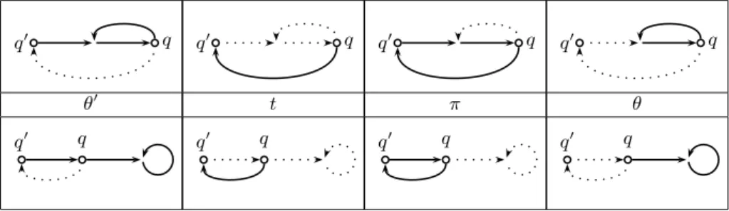
Proposition 4.2. Let t = (q, a, q′) be a transition and let θ′ be a simple fry-pan
starting from q′ such that the fry-pan tθ′ is not simple. In this case there exists a
minimal non-empty prefix π of tθ′ terminating in q. Moreover the fry-pan θ such
that tθ′ = πθ and the fry-pan πω are simple and such that Λ
r,m,a(λr,m(θ′)) ∈
q′ q q′ q q′ q q′ q
θ′ t π θ
q′ q q′ q q′ q q′ q
Fig. 2. A graphical support for Proposition 4.2 where θ′ denotes a simple
fry-pan starting from a state q′and t = (q, a, q′) is a transition such that the fry-pan
tθ′ is not simple. That means the state q is visited by θ′. Note that q is visited
either once or infinitely often. These two situations are depicted respectively on the top line and the bottom line of the tabular.
Proof. As tθ′ is not simple whereas θ′ is simple we deduce that there exists
a decomposition of tθ′ into πθ where π is the minimal non-empty prefix of tθ′
terminating in q. Let π be the non empty path with the minimal length. Observe that π is a simple cycle and thus πωis a simple fry-pan. Moreover, as θ is a suffix
of the simple fry-pan θ′, we also deduce that θ is a simple fry-pan. Observe that
λr,m(tθ′) = λr,m(πθ). Moreover, as π is a cycle in a m-graph we deduce that m
divides its length. Denoting by σ the label of π, we deduce that σ ∈ (Σm r )+.
Now, observe that Λr,m,σ(x) = (1 − r−
|σ|
m)λr,m(σω) + r− |σ|
mx for any x ∈ Rm.
We deduce that Λr,m,a(λr,m(θ′)) = (1 − r−
|σ|
m)λr,m(πω) + r− |σ|
mλr,m(θ). Thus
Λr,m,a(λr,m(θ′)) ∈ conv({λr,m(θ), λr,m(πω)}). ⊓⊔
From the previous Proposition 4.2 we deduce the following Proposition 4.3. Proposition 4.3. We have ΛG,m= conv(λr,m(ΘGS)).
We deduce that there exists a minimal finite set Λ0
G,m(q) ⊆ Qm such that
ΛG,m = conv(Λ0G,m). Note that an exhaustive computation of the whole set
ΘS
G(q) provides the set Λ0G,m(q) by removing vectors that are convex
combina-tion of others. The efficiency of such an algorithm can be greatly improved by computing inductively subsets Θ(q) ⊆ ΘS
G(q) and get rid of any fry-pan θ ∈ Θ(q)
as soon as it becomes a convex combination of other fry-pans in Θ(q)\{θ}. The algorithm Cycle is based on this idea.
Corollary 4.4. The algorithm Cycle(G,m) terminates by iterating the main while loop at most |T ||Q| times and it returns Λ0
G,m.
1 Cycle(G = (Q, Σr, T) be a m−graph, m ∈ N\{0})
2 foreach state q ∈ Q 3 ifΘSG(q) 6= ∅ 4 let θ ∈ ΘSG(q)
5 let Θ(q) ← {θ}
6 else
7 let Θ(q) ← ∅
8 whilethere exists t = (q, a, q′) ∈ T and θ′ ∈ Θ(q′) 9 such that Λr,m,a(λr,m(θ′)) 6∈ conv(λr,m(Θ(q)))
10 iftθ′ is simple
11 let Θ(q) ← Θ(q) ∪ {tθ′}
12 else
13 let π be the minimal strict prefix of tθ′ terminating in q 14 let θ be such that tθ′= πθ
15 let Θ(q) ← Θ(q) ∪ {θ, πω} 16 whilethere exists θ0∈ Θ(q)
17 such that conv(λr,m(Θ(q))) = conv(λr,m(Θ(q)\{θ0})) 18 let Θ(q) ← Θ(q)\{θ0}
19 returnλr,m(Θ) //Λ0G,m
5
Fix-point Computation
In this section we prove that the minimal post-fix-point ΓG,m(C0) is effectively
rational polyhedral for any m-graph G = (Q, Σr, T) and for any rational
poly-hedral initial valuation C0 ∈ Q → Cm. We deduce that the closed convex hull
of sets symbolically represented by arithmetic automata are effectively rational polyhedral.
Example 5.1. Let m = 1 and G = ({q}, Σr,{t}) where t = (q, r − 1, q) and
C0(q) = {0}. Observe that the sequence (Ci)i∈N where Ci+1 = Ci⊔ ΓG,m,t(Ci)
satisfies Ci(q) = {x ∈ R | 0 ≤ x ≤ ri− 1}.
Recall that a Kleene iteration algorithm applied on the computation of ΓG,m(C0) consists in computing the beginning of the sequence (Ci)i∈Ndefined by
the induction Ci+1= CiFt∈TΓG,m,t(Ci) until an integer i such that Ci+1= Ci
is discovered. Then the algorithm terminates and it returns Ci. In fact, in this
case we have Ci = ΓG,m(C0). However, as proved by the previous Example 5.1
the Kleene iteration does not terminate in general. Nevertheless we are going to compute ΓG,m(C0) by a Kleene iteration such that each Ciis safely enlarged into
a C′
i satisfying Ci ⊑ Ci′ ⊑ ΓG,m(C0). This enlargement follows the acceleration
framework introduced in [LS07b,LS07a] that roughly consists to compute the precise effect of iterating some cycles. This framework motivate the introduction of the monotonic function ΓW
G,m defined over the complete lattice (Q → Cm,⊑)
for any C ∈ Q → Cm and for any q ∈ Q by the following equality:
ΓG,mW (C)(q) =
G
q−→σ q
q CI,0(q) ΓGI,2(CI,0)(q) 1{(0, 0)} R+(1, 3) 2 ∅ (1, 1) + R+(3, 2) 3 ∅ R+(3, 2) 4 ∅ (1, 0) + R+(3, 2) 5 ∅ (0, 1) + R+(1, 3) 6 ∅ (2, 1) + R+(3, 2) 7 ∅ (0, 2) + R+(1, 3) 8 ∅ conv({(1, 0), (1, 2)}) + R+(1, 0) + R+(1, 3) 9 ∅ (0, 1) + R+(0, 1) + R+(3, 2)
Table 1. The values of CI,0 and CI = ΓGI,2(CI,0).
The following Proposition 5.2 shows that ΓW
G,m(C) is effectively computable
from C and the function ΛG,m introduced in section 3. In this proposition, Gq
denotes the graph G reduced to the strongly connected components of q. Proposition 5.2. For any C ∈ Q → Cm, and for any q ∈ Q, we have:
ΓG,mW (C)(q) = C(q) + R+(C(q) − ΛGq,m(q))
We now prove that the enlargement is sufficient to enforce the convergence of a Kleene iteration.
Proposition 5.3. Let C0⊑ C0′ ⊑ C1⊑ C1′ ⊑ . . . be the sequence defined by the
induction Ci+1 = Ci′
F
t∈TΓG,m,t(Ci′) and Ci′ = Γ W
G,m(Ci). There exists i < |Q|
satisfying Ci+1= Ci. Moreover, for such an integer i we have Ci= ΓG,m(C0).
Proof. Observe that Ci ⊑ Ci′ ⊑ ΓG,m(C0) for any i ∈ N. Thus, if there exists
i∈ N such that Ci+1 = Ci we deduce that Ci = ΓG,m(C0). Finally, in order to
get the equality C|Q| = C|Q|−1, just observe by induction over i that we have
following equality for any q2∈ Q:
Ci′(q2) = G q0−→σ1 q1−→σ q1−→σ2 q2 |σ1|+|σ2|≤i ΓG,m,σ1σσ2(C0(q1)) ⊓ ⊔ Example 5.4. Let us consider the 2-graph GIobtained from the 2-graph depicted
in the center of Fig. 1 and restricted to the set of states QI = {1, . . . , 9}. Let
us also consider the function CI,0∈ QI → C2 defined by CI,0(1) = {(0, 0)} and
CI,0(q) = ∅ for q ∈ {2, . . . , 9}. Computing inductively the sequence C0 ⊑ C0′ ⊑
C1 ⊑ C1′ ⊑ . . . defined in Proposition 5.3 from C0 = CI,0 shows that C6 = C5
(see section G in appendix). Moreover, this computation provides the value of CI = ΓGI,2(CI,0) (see Table 1).
1 FixPoint(G = (Q, Σr, T) a m−graph, m ∈ N\{0}, C0∈ Q → Cm)
2 let C ← C0
3 whilethere exists t ∈ T such that ΓG,m,t(C) 6⊑ C
4 C← ΓG,mW (C) 5 let C ← C ⊔F
t∈TΓG,m,t(C)
6 returnC
Corollary 5.5. The algorithm FixPoint(G,m,C0) terminates by iterating the
main while loop at most |Q|−1 times. Moreover, the algorithm returns ΓG,m(C0).
From Propositions 3.4 and 3.5 and corollaries 4.4 and 5.5 we get:
Theorem 5.6. The closed convex hull of sets symbolically represented by arith-metic automata are rational polyhedral and computable in exponential time. Example 5.7. We follow notations introduced in Examples 3.1, 3.2 and 5.4. Ob-serve that CI(8) − CD(a) = conv({(1, 0), (1, 2)}) + R+(1, 0) + R+(1, 3) is exactly
the closed convex hull of X = {x ∈ N2| 3x[1] > x[2]}.
6
Conclusion
We have proved that the closed convex hull of sets symbolically represented by arithmetic automata are rational polyhedral. Our approach is based on acceler-ation in convex data-flow analysis. It provides a simple algorithm for computing this set. Compare to [Lat04] (1) our algorithm has the same worst case expo-nential time complexity, (2) it is not limited to sets of the form Zm∩ C where
C is a rational polyhedral convex set, (3) it can be applied to any set defin-able in FO (R, Z, +, ≤, Xr), (4) it can be easily implemented, and (5) it is not
restricted to the most significant digit first decomposition. This last advantage directly comes from the class of arithmetic automata we consider. In fact, since the arithmetic automata can be non deterministic, our algorithm can be applied to least significant digit first arithmetic automata just by flipping the direc-tion of the transidirec-tions. Finally, from a practical point of view, as the arithmetic automata representing sets in the restricted logic FO (R, Z, +, ≤) (where Xr is
discarded) have a very particular structure, we are confident that the exponen-tial time complexity algorithm can be applied on automata with many states like the one presented in [Lat04]. The algorithm will be implemented in TaPAS [LP08] (The Talence Presburger Arithmetic Suite) as soon as possible.
References
BDEK07. Bernd Becker, Christian Dax, Jochen Eisinger, and Felix Klaedtke. Lira: Handling constraints of linear arithmetics over the integers and the reals. In Computer Aided Verification, 19th International Conference, CAV 2007, Berlin, Germany, July 3-7, 2007, Proceedings, volume 4590 of Lecture Notes in Computer Science, pages 307–310. Springer, 2007.
BH06. Bernard Boigelot and Fr´ed´eric Herbreteau. The power of hybrid accelera-tion. In Computer Aided Verification, 18th International Conference, CAV 2006, Seattle, WA, USA, August 17-20, 2006, Proceedings, volume 4144 of Lecture Notes in Computer Science, pages 438–451. Springer, 2006. BJW05. Bernard Boigelot, S´ebastien Jodogne, and Pierre Wolper. An effective
deci-sion procedure for linear arithmetic over the integers and reals. ACM Trans. Comput. Log., 6(3):614–633, 2005.
BLP06. S´ebastien Bardin, J´erˆome Leroux, and G´erald Point. Fast extended release. In Computer Aided Verification, 18th International Conference, CAV 2006, Seattle, WA, USA, August 17-20, 2006, Proceedings, volume 4144 of Lecture Notes in Computer Science, pages 63–66. Springer, 2006.
BRW98. Bernard Boigelot, St´ephane Rassart, and Pierre Wolper. On the expres-siveness of real and integer arithmetic automata (extended abstract). In Automata, Languages and Programming, 25th International Colloquium, ICALP’98, Aalborg, Denmark, July 13-17, 1998, Proceedings, volume 1443 of Lecture Notes in Computer Science, pages 152–163. Springer, 1998. FL05. Alain Finkel and J´erˆome Leroux. The convex hull of a regular set of integer
vectors is polyhedral and effectively computable. Information Processing Letter, 96(1):30–35, 2005.
Kar76. Michael Karr. Affine relationships among variables of a program. Acta Informatica, 6:133–151, 1976.
Lat04. Louis Latour. From automata to formulas: Convex integer polyhedra. In 19th IEEE Symposium on Logic in Computer Science (LICS 2004), 14-17 July 2004, Turku, Finland, Proceedings, pages 120–129. IEEE Computer Society, 2004.
Ler04. J´erˆome Leroux. The affine hull of a binary automaton is computable in polynomial time. In Verification of Infinite State Systems, 5th International Workshop, INFINITY 2003, Marseille, France, September 2, 2003, Proceed-ings, volume 98, pages 89–104. Elsevier, 2004.
Ler05. J´erˆome Leroux. A polynomial time presburger criterion and synthesis for number decision diagrams. In 20th IEEE Symposium on Logic in Com-puter Science (LICS 2005), 26-29 June 2005, Chicago, IL, USA, Proceed-ings, pages 147–156. IEEE Computer Society, 2005.
LP08. J´erˆome Leroux and G´erald Point. TaPAS : The Talence Presburger Arith-metic Suite. In Submited, 2008.
LS07a. J´erˆome Leroux and Gr´egoire Sutre. Accelerated data-flow analysis. In Static Analysis, 14th International Symposium, SAS 2007, Kongens Lyngby, Den-mark, August 22-24, 2007, Proceedings, volume 4634 of Lecture Notes in Computer Science, pages 184–199. Springer, 2007.
LS07b. J´erˆome Leroux and Gr´egoire Sutre. Acceleration in convex data-flow analy-sis. In FSTTCS 2007: Foundations of Software Technology and Theoretical Computer Science, 27th International Conference, New Delhi, India, De-cember 12-14, 2007, Proceedings, volume 4855 of Lecture Notes in Computer Science, pages 520–531. Springer, 2007.
Lug04. Denis Lugiez. From automata to semilinear sets: A logical solution for sets L(C, P). In Implementation and Application of Automata, 9th International Conference, CIAA 2004, Kingston, Canada, July 22-24, 2004, Revised Se-lected Papers, volume 3317 of Lecture Notes in Computer Science, pages 321–322. Springer, 2004.
Sch87. Alexander Schrijver. Theory of Linear and Integer Programming. John Wiley and Sons, New York, 1987.
A
Proof of Proposition 3.3
Proposition 3.3. The valuation ΛG,m is the unique minimal valuation C ∈
Q → Cm such that ΛG,m,t(C) ⊑ C for any transition t ∈ T and such that
C(q) 6= ∅ for any state q ∈ Q satisfying ΘG(q) 6= ∅.
Proof. Let us first prove that C = cl ◦ conv(λr,m(ΘG)) is a valuation in Q → Cm
such that ΛG,m,t(C) ⊑ C for any transition t ∈ T . We have the inclusion
Λr,m,a(λr,m(ΘG(q2))) ⊆ λr,m(ΘG(q1)) for any transition (q1, a, q2) ∈ T . As
cl ◦ conv and Λr,m,a are commutative, the valuation C = cl ◦ conv(λr,m(ΘG))
satisfies ΛG,m,t(C) ⊑ C for any transition t ∈ T .
Now, let us consider a valuation C ∈ Q → Cm such that ΛG,m,t(C) ⊑ C
for any transition t ∈ T and such that C(q) 6= ∅ for any state q ∈ Q satisfying ΘG(q) 6= ∅. Let us prove that cl ◦ conv(λr,m(ΘG)) ⊑ C. As ΛG,m,t(C) ⊑ C for
any transition t ∈ T an immediate induction shows that Λr,m,σ(C(q)) ⊑ C(q′)
for any finite path π = (q−→ qσ ′). Let us consider an infinite path θ = (q w
−→ F ). As F is non empty, there exists a state q′∈ F . Recall that F is the set of states
visited infinitely often by the path θ. We deduce that there exists a cycle on q′
and in particular ΘG(q′) 6= ∅. This condition implies C(q′) 6= ∅. Thus there exists
x′∈ C(q′). Moreover, as q′ is visited infinitely often by θ, there exists a strictly
increasing sequence 0 ≤ i0< i1<· · · of integers such that q
w(1)...w(ij)
−−−−−−−→ q′. This
path shows that the vector xj = Λr,m,w(1)...w(ij)(x
′) is in C(q). As lim
j→+∞xj=
λr,m(w) and C(q) is closed we deduce that λr,m(w) ∈ C(q). We have proved that
B
Proof of Lemma 4.1
Lemma 4.1. λr,m(σω) is the unique fix-point of Λr,m,σ for any σ ∈ Σr+.
Proof. As σσω and σω are equal, equality (1) page 7Reduction to Data-Flow
Analysis Problemsequation.1 shows that λr,m(σω) is a fix-point of Λr,m,σ.
More-over as the uniform form of the linear function Λr,m,ais equal to Λr,m,0we deduce
that the uniform form of Λm
r,m,σ is equal to Λ m|σ|
r,m,0. Since Λmr,m,0(x) = r−1xwe
have proved that the uniform form of Λm
r,m,σ is x → r−|σ|x for any x ∈ Rm.
Moreover, as λr,m(σω) is a fix-point of Λmr,m,σ we deduce that Λmr,m,σ(x) =
λr,m(σω) + r−|σ|(x − λr,m(σω)) for any x ∈ Rm. In particular, if x is a
fix-point of Λr,m,σ, we get x = λr,m(σω) + r−|σ|(x − λr,m(σω)). As r−|σ| 6= 1 we
C
Proof of Proposition 4.3
Proposition 4.3. We have ΛG,m= conv(λr,m(ΘSG)).
Proof. From ΘS
G(q) ⊆ ΘG(q) we deduce the inclusion conv(λr,m(ΘGS)) ⊆ ΛG,m.
Let us prove the other inclusion. Observe that ΘS
G(q) is a finite set and in
par-ticular conv(ΘS
G(q)) is a closed convex set for any q ∈ Q. Let us consider the
function C ∈ Q → Cm defined by C = conv(λr,m(ΘGS)). From Proposition 4.2,
we deduce that ΛG,m,t(C) ⊑ C for any transition t ∈ T . Note also that C(q) 6= ∅
for any state q ∈ Q such that ΘG(q) 6= ∅. By minimality of ΛG,m we get the
D
An Additional Example For Section 4
q ΘS G1(q) −Λ 0 G1,2(q) 1 (00)ω,(0111)ω,01(0010)ω,0100(11)ω {(0, 0), (1 3,1))} 2 1(00)ω ,(1011)ω ,101(0010)ω ,10100(11)ω {(1 2,0), ( 7 8, 1 4))} 3 (1110)ω,100(11)ω,1(0010)ω {(1,2 3), ( 1 2, 1 3)} 4 0(11)ω,(0100)ω,01011(00)ω,010(1101)ω {(1 2,1),{(0, 2 3)} 5 11(00)ω,(1101)ω,(0010)ω,00(11)ω {(2 3,1), ( 1 3,0)} 6 (11)ω,(0001)ω,0(1101)ω,011(00)ω {(1, 1), (0,1 3)} 7 (11)ω ,(1000)ω ,10(1101)ω ,1011(00)ω {(2 3,0), (1, 1)} Table 2. Some values computed9 8 0 1 1 1 3 0 2 1 0 0 5 1 -2 -1 0 1 4 0 6 0 7 1 1 0 0 0 * 0 1 a * b 0 0
Fig. 3. An arithmetic automaton in basis 2 and in dimension 2.
Example D.1. Let us consider the 2-graph G labelled by Σ2 and depicted in
Fig. 3. We denote by G1 the graph G restricted to the strongly connected
com-ponent {1, . . . , 7}. By enumerating all the possible simple fry-pans ΘS
G1(q)
start-ing from a state q, observe that we get the values given in the Table 2. This table only provides the labels of the fry-pans in order to simplify the presenta-tion. However, the fry-pans can be recovered from their labels since the graph is deterministic.
E
Proof of Corollary 4.4
Corollary 4.4. The algorithm Cycle(G,m) terminates by iterating the main while loop at most |T ||Q| times and it returns Λ0
G,m.
Proof. Observe that Θ(q) ⊆ ΘS
G(q) for any state q at any step of the algorithm.
Moreover, each time the while loop is executed, the set C(q) = conv(λr,m(Θ(q)))
strictly increases. Thus, the set {θ ∈ ΘS
G(q) | λr,m(θ) ∈ C(q)} strictly increase
each time the while loop is executed. Observe that a simple fry-pan θ is uniquelly determined from its |Q| first transitions. ThusP
q∈Q|Θ S
G(q)| ≤ |T ||Q|. We deduce
that the algorithm terminates after executing at most |T ||Q|times the while loop.
Finally, let us prove that when the algorithm terminates it returns Λ0
G,m. It is
sufficient to show that C = ΛG,mwhen it terminates. Note that the while loop
condition is no longer valid. Thus ΛG,m,t(C) ⊑ C for any transition t ∈ T . As
C(q) 6= ∅ for any state q ∈ Q such that ΘG(q) 6= ∅, by minimality of ΛG,m we
deduce that ΛG,m ⊑ C. Thus C = ΛG,m when the algorithm terminates. We
deduce that the algorithm returns Λ0
F
Proof of Proposition 5.2
We first prove the following two technical lemmas. Lemma F.1. For any σ ∈ (Σm
r )+ and for any x ∈ R
m we have:
cl ◦ conv({Γr,m,σi(x) | i ∈ N}) = x + R+(x − λr,m(σω))
Proof. As λr,m(σω) is a fix-point of the linear function Γr,m,σiand as the uniform
form of the linear function Γr,m,σi is Γr,m,0i|σ| , we deduce that Γr,m,σi(x) = x +
(ri|σ|m − 1)(x − λ
r,m(σω)) for any i ∈ N. As cl ◦ conv({ri
|σ|
m − 1 | i ∈ N}) = R+
we deduce the lemma. ⊓⊔
Lemma F.2. For any strongly connected m-graph G = (Q, Σr, T) and for any
state q ∈ Q, we have : ΛG,m(q) = cl ◦ conv({λr,m(σω) | q σ∈(Σm r ) + −−−−−−→ q}) Proof. Let C(q) = cl ◦ conv({λr,m(σω) | q
σ∈(Σm r )+
−−−−−−→ q}) be defined for any q ∈ Q. Note that for any cycle π = (q σ∈(Σ
m r)+
−−−−−−→ q) we have πω ∈ Θ
Gq(q). In
particular λr,m(σω) ∈ ΛG,m(q). We deduce the inclusion C(q) ⊑ ΛG,m(q). For
the other inclusion, let us consider an infinite path q−w→ F and let q′∈ F . Since
F is the set of states visited infinitely often, there exists a strictly increasing sequence of integers 0 < i0 < i1 < · · · such that q
w(1)...w(ij)
−−−−−−−→ q′ for any
integer j ≥ 0. As G is strongly connected, there exists a path q′ σ
−→ q. The cycle q w(1)...w(ij)σ
−−−−−−−−→ q shows that the vector xj = λr,m((w(1) . . . w(ij)σ)ω) is
in C(q). As limj→+∞xj = λr,m(w) and C(q) is closed we have proved that
λr,m(w) ∈ C(q). Thus ΛG,m(q) ⊑ C(q). ⊓⊔
Proposition 5.2. For any C ∈ Q → Cm, and for any q ∈ Q, we have :
ΓG,mW (C)(q) = C(q) + R+(C(q) − ΛGq,m(q))
Proof. Note that if there does not exist a q −→ q then Λσ Gq,m(q) = ∅ and the
previous equality is immediate. Otherwise, from Lemmas F.1 and F.2 we get the following equalities: ΓG,mW (C)(q) = G q−→σ q Γr,m,σ(C(q)) = G x∈C(q) G q σ∈(Σmr )+ −−−−−−→q cl ◦ conv({Γr,m,σi(x) | i ∈ N}) = G x∈C(q) G q σ∈(Σmr ) + −−−−−−→q x+ R+(x − λr,m(σω)) = G x∈C(q) x+ R+(x − ΛGq,m(q))
In particular we deduce that ΓW
G,m(C)(q) ⊑ C(q) + R+(C(q) − ΛGq.m(q)).
Con-versely, let us consider x ∈ C(q) + R+(C(q) − ΛGq,m(q)). The vector x can be
decomposed into x = c1+ h(c2− z) where c1, c2 ∈ C(q), z ∈ ΛGq,m(q) and
h∈ R+. Let us denote by c = 1+h1 (c1+ hc2). As C(q) is convex we deduce that
c∈ C(q). From x = c + h(c − z) we deduce that x ∈ ΓW
![Fig. 1. On the left, the rational polyhedral convex set C = {x ∈ R 2 | 3x[1] >](https://thumb-eu.123doks.com/thumbv2/123doknet/14440975.516924/5.892.260.666.517.791/fig-left-rational-polyhedral-convex-set-c-r.webp)