Coherent control of electron spins in diamond for quantum information science and quantum sensing

Coherent control of electron spins in diamond for

quantum information science and quantum sensing

by

Alexandre Cooper-Roy

B.Eng., École Polytechnique de Montréal (2008)

Ingénieur Polytechnicien, École Polytechnique (2009)

M.Eng., The University of Tokyo (2010)

Submitted to the Department of Nuclear Science and Engineering

in partial fulfillment of the requirements for the degree of

Doctor of Philosophy

at the

MASSACHUSETTS INSTITUTE OF TECHNOLOGY

September 2016

c

○ Massachusetts Institute of Technology 2016. All rights reserved.

Author . . . .

Department of Nuclear Science and Engineering

July 22nd, 2016

Certified by. . . .

Paola Cappellaro

Associate Professor

Thesis Supervisor

Accepted by . . . .

Ju Li

Chairman, Department Committee on Graduate Theses

Coherent control of electron spins in diamond for quantum

information science and quantum sensing

by

Alexandre Cooper-Roy

Submitted to the Department of Nuclear Science and Engineering on July 22nd, 2016, in partial fulfillment of the

requirements for the degree of Doctor of Philosophy

Abstract

This thesis introduces and experimentally demonstrates coherent control techniques to exploit electron spins in diamond for applications in quantum information process-ing and quantum sensprocess-ing. Specifically, optically-detected magnetic resonance mea-surements are performed on quantum states of single and multiple electronic spins associated with nitrogen-vacancy centers and other paramagnetic centers in synthetic diamond crystals.

We first introduce and experimentally demonstrate the Walsh reconstruction method as a general framework to estimate the parameters of deterministic and stochastic fields with a quantum probe. Our method generalizes sampling techniques based on dynamical decoupling sequences and enables measuring the temporal profile of time-varying magnetic fields in the presence of dephasing noise.

We then introduce and experimentally demonstrate coherent control techniques to identify, integrate, and exploit unknown quantum systems located in the environment of a quantum probe. We first locate and identify two hybrid electron-nuclear spins systems associated with unknown paramagnetic centers in the environment of a single nitrogen-vacancy center in diamond. We then prepare, manipulate, and measure their quantum states using cross-polarization sequences, coherent feedback techniques, and quantum measurements. We finally create and detect entangled states of up to three electron spins to perform environment-assisted quantum metrology of time-varying magnetic fields. These results demonstrate a scalable approach to create entangled states of many particles with quantum resources extracted from the environment of a quantum probe. Applications of these techniques range from real-time functional imaging of neural activity at the level of single neurons to magnetic resonance spec-troscopy and imaging of biological complexes in living cells and characterization of the structure and dynamics of magnetic materials.

Thesis Supervisor: Paola Cappellaro Title: Associate Professor

Acknowledgments

This thesis has been made possible by the financial support from the Fulbright Scholar Program and the Natural Sciences and Engineering Research Council of Canada. A very special thank you goes to all of my mentors, colleagues, and friends at MIT, Harvard, and elsewhere in the world who have helped me become the person I am today.

First and foremost, Professor Paola Cappellaro has been very keen on supervising my research activities and guiding my scientific growth during my tenure within her group. Paola has provided me with a tremendous amount of freedom to explore cre-ative approaches to identifying and solving problems in science and engineering. She has always been very open to discuss new ideas and provide feedback on my progress towards reaching my goals. Paola is a very dedicated and thoughtful mentor with an inspiring motivation to better understand the quantum world and a great ability to combine a deep understanding of theoretical concepts with insightful experimental evidences.

Professor Ju Li has provided me with many valuable advice as the chairman of the committees of both my qualifying exam and my thesis defense, including the importance of making connections with the work of others and focusing on solutions that enable discoveries and new technologies.

Professor Dirk Englund has provided me with many valuable advice about my scientific research and career goals as an academic advisor and member of my thesis committee. I very much admire the ability of Dirk to carry out collaborative re-search projects on multidisciplinary fronts at the confluence of scientific disciplines and thank him for providing me with such great opportunities to learn from the numerous members of his group.

Professor Ronald Walsworth from the Center for Astrophysics (CFA) at Har-vard University has been an inspiring role model who taught me by example about the importance and excitement of building strong collaborative teams and tackling challenging problems at the intersection of multiple fields of research. Ron has

sig-nificantly contributed to the success of my research by encouraging me to attend his group meetings and exchange (classical) information and matter with his postdocs and students.

Professor Ed Boyden from the Media Lab at MIT has taught me through many intense discussions about the importance of maximizing impact by solving the most important problems facing humanity, identifying valuable opportunities by using a wide variety of cognitive tools, and maintaing strong collaborative ties with experts across disciplines.

Many other professors have also helped shaping my scientific growth, including Professors Lorenza Viola from Dartmouth University, Dmitry Pushin from University of Waterloo, Nir Bar-Gill from the Hebrew University of Jerusalem, and Michael Biercuk from the University of Sydney.

Second, I would like to acknowledge the help and friendship of all of the postdocs that have spent time with me discussing about Science, have taught me experimental skills and theoretical concepts, and have encouraged my quest for knowledge with key insights and pieces of equipment.

HoNam Yum has taught me valuable experimental skills in optics and electronics as we worked together on designing and building our first confocal microscope.

Easwar Magesan has cheerfully joined my efforts to work out the theory of the Walsh reconstruction method and compressed sensing approach to quantum param-eter estimation. Easwar’s enthusiasm for solving tough mathematical problems has positively influenced my approach to research.

Gerardo Paz-Silva from Dartmouth University has taught me a lot about noise spectroscopy and the Magnus expansion during many of our visits and video calls.

Chinmay Belthangady from Walsworth group at Harvard has spent a great deal of his time at MIT to help me set up the electronics for driving electron spins in diamond as we launched our new project on environment-assisted quantum metrology. Chinmay’s positive and generous attitude has inspired me to become a better person. Huiliang Zhang from Walsworth group at Harvard has answered many of my questions about diamond fabrication and has patterned and implanted the diamond

sample in which we ended up identifying two unknown paramagnetic centers.

Many other postdocs have contributed to my theoretical and experimental research work. David Gelbwaser from Aspuru-Guzik group at Harvard has spent many hours with me discussing about quantum thermodynamics and the efficiency of quantum engines. Jean-Christophe Jaskula has taught me about super-resolution microscopy and has helped me resolving technical issues with our confocal microscope. Luca Marseglia has helped out fabricating new coplanar waveguides and acid cleaning our diamond samples. David Le Sage taught me about aligning an acousto-optic mod-ulator in the bow-tie configuration. David Glenn has provided me with technical guidance in building our first confocal microscope and has fueled my interest in bio-physics. Alexei Trifonov has helped diagnosing issues in our optical setup. Linh Pham has answered many of my questions about handling diamond samples and perform-ing magnetometry experiments; her lablog posts have always been a great source of inspiration. Ulf Bissbort has taught me about solving algebraic expressions in spin physics using the C programming language. Kasturi Saha has helped fixing issues in our optical setup. Gurneet Kaur has provided me with great advice about recording scientific information and experimental measurements.

Third, I would like to acknowledge the friendship of my student colleagues from the Quantum Engineering Group, which have played an important role in shaping my experience at MIT.

Clarice Aiello wrote the first version of our control software and provided valuable support in designing and building our control electronics to manipulate the quantum state of single nitrogen-vacancy centers in diamond.

Masashi Hirose provided me with the source code to simulate the dynamics of confined ensembles of interacting electron spins and engaged me in many discussions about understanding new sets of experimental data.

Ashok Ajoy provided support on automating the alignment of the static magnetic field and contributed to many discussions on performing spectral measurements on ensembles of electron spins.

Hamil-tonian of multi-resonance pulse sequences and engaged me in many interesting dis-cussions about many-body physics and nonequilibrium spin dynamics.

Akira Sone stimulated my interest in algebraic geometry during many interesting discussions about his projects on system identification. Calvin Sun and Mo Chen have helped me upgrading our experimental system and took over the measurements after my departure to Caltech. Yixiang Liu has helped me simulating the implantation profile of nitrogen ions in diamond. Gary Wolfowicz, Joe Smith and Scott Alsid has brought great energy to our group and positively contributed to its cohesion.

I would also like to thank my student colleagues from the Walsworth group for invaluable discussions, including Emma Rosenfeld, Paul Junghyun Lee, Erik Bauch, and Keigo Arai; my student colleagues from the Dirk’s group, especially Edward Chen who helped me upgrading our confocal microscope and leading the iQuISE student program and Matt Trusheim who provided answers to my questions about diamond fabrication; Jonathan Welch from Asupuru-Guzik’s group who encouraged my study of Walsh analysis; and my friends from the iQuISE leadership team, especially Kristin Beck, Zheshen Zhang, and Sara Mouradian. I would also like to thank my friends from Boston Team Handball, especially Nader Shaar who acted as a great personal mentor. Special thanks go to Laura von Bosau, Teresa Avila, Heather Barry and Clare Egan for administrative support and Kurt Broderick for technical support in the clean room.

Finally, I would like to thank my family, my parents, and my wife for their care, support, and kind devotion. Thank you very much!

Contents

1 Introduction 13

1.1 Conceptual framework . . . 14 1.2 Outline of this thesis . . . 15 2 Time-resolved magnetic sensing with electronic spins in diamond 17 2.1 Quantum parameter estimation with quantum probes . . . 19 2.1.1 Understand the Walsh reconstruction method . . . 21 2.1.2 Quantify the performance of the Walsh reconstruction method 24 2.2 Demonstrate the Walsh reconstruction method experimentally with a

single nitrogen-vacancy center in diamond . . . 34 2.2.1 Reconstruct the temporal profile of sinusoidal fields . . . 34 2.2.2 Reconstruct the temporal profile of bichromatic fields . . . 37 2.2.3 Reconstruct the temporal profile of arbitrary time-varying fields 38 2.3 Conclusion and outlook . . . 42 2.3.1 Comparison with existing techniques . . . 42 2.3.2 Applications to sensing neural activity . . . 44 3 Spectral reconstruction of stochastic fields with Walsh sequences 47 3.1 Noise spectroscopy with single quantum probes . . . 47 3.1.1 Discrete representation of the autocorrelation function . . . . 50 3.1.2 Continuous representation of the autocorrelation function . . . 54

4 Environment-assisted quantum metrology with entangled states of

electron spins in diamond 61

4.1 Quantum system identification . . . 63 4.1.1 Identify two unknown paramagnetic centers in the environment

of a single nitrogen-vacancy center in diamond . . . 63 4.1.2 Estimate the parameters of the internal spin Hamiltonian of

two unknown paramagnetic centers in diamond . . . 65 4.2 Quantum system integration . . . 74 4.2.1 Initialize quantum systems using coherent feedback control . . 74 4.2.2 Initialize quantum systems using cross-polarization . . . 83 4.3 Quantum system exploitation . . . 89 4.3.1 Understand entangled states of electron spins . . . 89 4.3.2 Create and detect entangled states of two electron spins . . . . 97 4.3.3 Create and detect entangled states of three electron spins . . . 99 4.3.4 Measure magnetic fields with entangled states of electron spins 101 4.3.5 Perform repetitive quantum measurements of electron spins . 104 4.4 Conclusion and outlook . . . 108

List of Figures

1-1 Understand the conceptual framework underlying this thesis. . . 15

2-1 Understand the Walsh reconstruction protocol. . . 18

2-2 Understand the Walsh functions. . . 20

2-3 Simulate the reconstruction of bichromatic fields. . . 31

2-4 Quantify the accuracy of the Walsh reconstruction method. . . 32

2-5 Reconstruct sinusoidal fields with Walsh sequences. . . 35

2-6 Extract the Walsh coefficient from the fluorescence signal. . . 36

2-7 Reconstruct bichromatic fields with Walsh sequences. . . 37

2-8 Characterize the transmission properties of the coplanar waveguide. . 38

2-9 Simulate an action potential. . . 40

2-10 Reconstruct arbitrary time-varying fields with Walsh sequences. . . . 41

3-1 Represent two-dimensional Walsh filters (1). . . 51

3-2 Represent two-dimensional Walsh filters (2). . . 52

3-3 Represent the arithmetic and dyadic sampling domain. . . 54

3-4 Represent the autocorrelation function of a stationary process. . . 55

3-5 Represent the arithmetic and dyadic sampling domain. . . 56

4-1 Measure the resonance spectrum of two paramagnetic centers. . . 64

4-2 Observe from above the Terra-B diamond sample. . . 66

4-3 Estimate the strength and orientation of the static magnetic field. . . 69

4-4 Measure the cw-esr spectrum of an ensemble of NV centers. . . 70

4-6 Estimate the dipolar components of two paramagnetic centers. . . 72

4-7 Initialize quantum systems using coherent feedback control. . . 78

4-8 Initialize quantum systems using cross-polarization in the rotating frame. 84 4-9 Understand cross-polarization in the rotating frame. . . 85

4-10 Initialize an electron spin using Hartmann-Hahn cross-polarization. . 87

4-11 Initialize another electron spin using Hartmann-Hahn cross-polarization. 88 4-12 Create entangled states of two electron spins in diamond. . . 98

4-13 Detect entangled states of two electron spins in diamond. . . 100

4-14 Create entangled states of three electron spins in diamond. . . 101

4-15 Detect entangled states of three electron spins in diamond. . . 102

4-16 Measure magnetic fields with entangled states of two electron spins. . 103

4-17 Perform repetitive readout of a single electron spin. . . 105 4-18 Detect entangled states of two electron spins using repetitive readout. 107

Chapter 1

Introduction

Quantum systems composed of many interacting particles of light and matter exhibit complex dynamical properties that can be studied experimentally to better under-stand fundamental states of matter and design novel technologies. Coherent control techniques to prepare, manipulate, and read out the quantum state of single and mul-tiple interacting quantum systems have been demonstrated in a vast array of physical systems, including superconducting qubits, trapped ions, quantum dots, ultracold atoms in optical lattices, electron donors in semiconductors, and spin defects in solid-state materials. Spin defects in solid-solid-state materials are particularly promising for applications in quantum metrology and sensing; in particular, electron and nuclear spins associated with single and multiple nitrogen-vacancy (NV) centers in diamond have recently been used as quantum probes to measure the spatiotemporal profile of electric and magnetic fields associated with molecular and biological samples at the atomic scale under ambient conditions.

Quantum metrology explores quantum strategies such as the use of entanglement, discord, and squeezing to reduce the statistical error associated with the estimation of unknown physical parameters. Environment-assisted metrology exploits the environ-ment of a quantum sensor to estimate unknown parameters with an improveenviron-ment in precision beyond the limits allowed by classical strategies. Quantum strategies that outperform classical strategies have been explored in different physical implementa-tions of a quantum probe to improve the performance of metrology tasks, including

squeezed states, non-Gaussian spin states, and entangled states of many quantum particles. The creation of multipartite entangled states of electron spins in solid-state materials has been hindered, however, by the difficulty of initializing their quantum state in a state of low entropy and protecting their evolution against dephasing in the presence of environmental fluctuations.

This thesis makes significant contributions to quantum metrology in two important areas. First, we extend the framework of quantum parameter estimation to estimate deterministic and stochastic time-dependent parameters. Our approach takes advan-tage of the Walsh functions to generate a complete set of digital filters that efficiently sample and reconstruct time-varying fields. Second, we develop coherent control tech-niques to extract quantum resources from the environment of a quantum probe to create entangled states of many quantum particles and perform environment-assisted quantum metrology. These techniques are experimentally demonstrated with hybrid electron-nuclear spin systems associated with unknown paramagnetic centers located in the environment of a single nitrogen-vacancy center in diamond.

1.1 Conceptual framework

The conceptual framework underlying this thesis is the coherent control of open quan-tum systems for applications in quanquan-tum metrology and sensing (Fig. 1-1). Coherent control techniques are introduced to control and characterize the dynamics of open quantum systems, specifically composed of a single quantum probe interacting with an environment formed by a mesoscopic ensemble of interacting quantum particles, such as electron spins in diamond. The goal is not only to characterize the influence of the environment on the evolution of a quantum probe, but also to exploit the quan-tum properties of the environment in order to improve the performance of quanquan-tum metrology protocols. We introduce and experimentally demonstrate coherent con-trol techniques to prepare, manipulate, and measure the quantum state of unknown paramagnetic centers located in the environment of a single NV center in diamond. We then convert these unknown paramagnetic centers into quantum resources useful

E

E

E

S

a

_b

c

_d

E

E

E

S

E

E

E

S

E

E

E

S

Figure 1-1: Coherent control of open quantum systems for applications in quantum information science and quantum sensing. a, A single quantum probe interacts with many fragments of its environment, causing the decay of coherent superposition of states and preventing interferometric measurements of time-varying fields over long periods of time. b, Coherent control sequences applied on the quantum probe decouple the quantum probe from its environment, increasing the lifetime of coherent superposition of states and enabling interferometric measurements of time-varying fields over long periods of time. c, Coherent control sequences simultaneously applied on both the quantum probe and a resonant fragment of its environment selectively recouple their mutual interaction, thus providing information about the structure and dynamics of the environment. d, A single quantum probe converts a fragment of its environment into quantum resources useful for creating entangled states of many particles and performing interferometric measurements of time-varying fields with improved sensitivity.

for creating entangled states of multiple electron spins and measuring time-varying fields with improved sensitivity. Performing repetitive quantum measurements of the quantum state of the electron spins provides a gain in information that balances the detrimental effects of control errors and dissipation during quantum operations and quantum evolution.

1.2 Outline of this thesis

This thesis addresses the problem of measuring deterministic and stochastic fields with single quantum probes in Chapter 2 and Chapter 3, before tackling the problem

of converting unknown quantum systems into quantum resources useful for quantum sensing in Chapter 4.

Chapter 2 introduces the Walsh reconstruction method [15, 16, 17], which is a new approach to quantum parameter estimation based on Walsh sequences that si-multaneously extract information about time-varying fields and suppress dephasing due to incoherent sources of noise. We experimentally demonstrate the Walsh recon-struction method by measuring the temporal profile of various time-varying magnetic fields, including the magnetic field created by an action potential traveling throught the physical model of a neuron.

Chapter 3 extends the Walsh reconstruction method to the problem of estimating the parameters of stochastic fields. The Walsh spectroscopy method samples the noise spectrum in the sequency domain and synthesizes the autocorrelation function in the time domain using a series of linear transformations without the need for solving a deconvolution problem.

Chapter 4 addresses the problem of converting unknown quantum systems in the environment of a quantum probe into quantum resources useful for quantum metrology and sensing. Magnetic double-resonance techniques are introduced and exploited to locate and identify unknown paramagnetic centers in the environment of a single NV center in diamond. These paramagnetic centers are hybrid electron-nuclear spin systems characterized by a single electron spin interacting with a single nuclear spin. The parameters of the magnetic dipolar interaction terms and hyperfine interaction terms are estimated by varying the strength and orientation of the static magnetic field. After initializing the quantum state of multiple electron spins using cross-polarization sequences and coherent feedback techniques, entangled states of two and three electron spins are created to perform a.c. magnetometry, i.e., estimate the amplitude of sinusoidal magnetic fields.

Chapter 5 summarizes the main scientific and technical contributions of this thesis and discusses approaches to develop new technologies in quantum metrology and sensing and solve fundamental problems in many-body quantum physics.

Chapter 2

Time-resolved magnetic sensing with

electronic spins in diamond

Quantum probes measure time-varying fields with high sensitivity and spatial res-olution, enabling the study of biological, material, and physical phenomena at the nanometer scale. In particular, NV centers in diamond have recently emerged as promising quantum probes for measuring magnetic [1, 2, 3] fields, electric [4] fields, and temperature [5, 6, 7]. These sensors are ideal for nanoscale imaging of living bio-logical systems [8, 9, 10] due to their low cytotoxicity, surface functionalizations [11], optical trapping capability [12, 13] and long coherence time under ambient condi-tions [14].

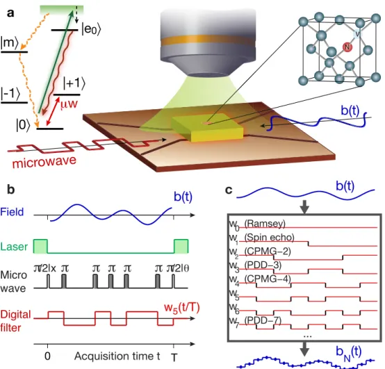
Although coherent control techniques have measured the amplitude of constant or oscillating fields, these techniques are not suitable for measuring time-varying fields with unknown dynamics. In this chapter, we introduce a coherent acquisition method (Fig. 2-1) to accurately reconstruct the temporal profile of time-varying fields using Walsh sequences [15, 16, 17]. These decoupling sequences act as digital filters that efficiently extract spectral coefficients while suppressing decoherence, thus providing an improved sensitivity over existing strategies. We experimentally reconstruct the temporal profile of the time-varying magnetic field radiated by a physical model of a neuron using a single electron spin in diamond.

N V

|e

〉

|+1

〉

|-1

〉

|m

〉

|0

〉

|+1

μw

microwave

b(t)

a

b

π

π

π π π

π

π

b(t)

b(t)

b

(t)

c

Figure 2-1: Understand the Walsh reconstruction protocol. a, A single nitrogen-vacancy (NV) center in diamond, optically initialized and read out by confo-cal microscopy, is manipulated with coherent control sequences to measure the arbi-trary profile of time-varying magnetic fields radiated by a coplanar waveguide under ambient conditions. b, Coherent control sequences, acting as digital filters on the evolution of the qubit sensor, extract information about time-varying fields. c, An 𝑁-point functional approximation of the field is obtained by sampling the field with a set of 𝑁 digital filters taken from the Walsh basis, which contain some known set of decoupling sequences such as the even-parity Carr-Purcell-Meiboom-Gill (CPMG) sequences [18] (𝑤2𝑛) and the odd-parity Periodic Dynamical Decoupling (PDD)

2.1 Quantum parameter estimation with quantum

probes

Measurements of weak electric and magnetic fields at the nanometer scale are in-dispensable in many areas, ranging from materials science to fundamental physics and biomedical science. In many applications, much of the information about the underlying phenomena is contained in the dynamics of time-varying fields. While novel quantum probes promise to achieve the required combination of high sensitiv-ity and spatial resolution, their application to efficiently mapping the temporal profile of time-varying fields is still a challenge.

Quantum estimation techniques [20] measure time-varying fields by monitoring the shift in the resonance energy of a quantum probe, e.g., via Ramsey interferome-try. The quantum probe, first prepared in an equal superposition of its eigenstates, accumulates a phase 𝜑(𝑇 ) = 𝛾 ∫︀𝑇

0 𝑏(𝑡)𝑑𝑡, where 𝛾 is the strength of the interaction with the time-varying field 𝑏(𝑡) during the acquisition period 𝑇 .

The dynamics of time-varying fields could be mapped by measuring the quantum phase over successive, increasing acquisition periods [14] or sequential small acquisi-tion steps [21]; however, these protocols are inefficient at sampling and reconstructing time-varying fields, as the former involves a deconvolution problem, while both are limited by short coherence times (𝑇*

2) that bound the measurement sensitivity. Decou-pling sequences [18, 22, 19] could be used to increase the coherence time [23, 24, 25], but their application would result in a non-trivial encoding of the dynamics of the field onto the phase of the qubit sensor [26, 27, 28, 29, 30].

Instead, here we propose to reconstruct the temporal profile of time-varying fields with a set of digital filters, implemented with coherent control sequences over the whole acquisition period 𝑇 , that simultaneously extract information about the dy-namics of time-varying fields and protect the evolution of the qubit sensor against dephasing noise. In particular, we use control sequences (Fig. 2-2) associated with the Walsh functions [31], which form a complete orthonormal basis of digital filters and are easily implementable experimentally.

Ramsey w₀ Spin echo w₁ = r₁ CPMG-2 w₂ PDD-3 w₃ = r₂ CPMG-4 w₄ w₅ w₆ PDD-7 w₇ = r₃ CPMG-8 w₈ w₉ w₁₀ w₁₁ w₁₂ w₁₃ w₁₄ PDD-15 w15 = r4 1 3 7 15 1 3 7 15 1 3 7 15 a b c d

Figure 2-2: Understand the Walsh functions. Matrix representation of the Walsh functions up to fourth order (𝑁 = 24_{) in a, sequency ordering, b, Paley ordering, and} c, Hadamard ordering. Each line corresponds to a Walsh sequence with the columns giving the value of the digital filter in the time domain. Black and white pixels represent the values ±1. Each ordering can be obtained from the others by linear transformations. d Walsh functions {𝑤𝑚}𝑁 −1𝑚=0 up to 𝑁 = 24 in sequency ordering. The sequency 𝑚 indicates the number of zero crossings of the 𝑚-th Walsh function. The Rademacher functions 𝑟𝑘 = 𝑤2𝑘₋₁ correspond to the Walsh functions plotted in

blue. Some Walsh functions are associated with known decoupling sequences such as the even-parity CPMG sequences [18] (𝑤2𝑘 green lines) and the odd-parity PDD

The Walsh reconstruction method uses a complete set of digital filters, imple-mented with coherent control sequences over the acquisition period 𝑇 , to simulta-neously extract information about the dynamics of time-varying fields and protect the evolution of the quantum probe against dephasing noise. The Walsh reconstruc-tion method can be applied to estimate various time-varying parameters via coherent control of any quantum probe. In particular, we show that the phase acquired by a qubit sensor modulated with Walsh decoupling sequences is proportional to the Walsh transform of the field. This simplifies the problem of spectral sampling and re-construction of time-varying fields by identifying the sequency domain as the natural description for dynamically modulated quantum systems.

At the same time, the Walsh reconstruction method provides a solution to the problem of monitoring time-dependent parameters with a quantum probe, which in general cannot be achieved via continuous tracking due to the destructive nature of quantum measurements. In addition, because the Walsh reconstruction method achieves dynamical decoupling of the quantum probe, it further yields a significant improvement in coherence time and sensitivity over sequential acquisition techniques. These characteristics and the fact that the Walsh reconstruction method can be com-bined with data compression [16] and compressive sensing [17, 32] provide clear ad-vantages over prior reconstruction techniques [14, 21, 33, 34].

2.1.1 Understand the Walsh reconstruction method

The Walsh reconstruction method relies on the Walsh functions (Fig. 2-2), which are a family of piecewise-constant functions taking binary values, constructed from products of square waves, and forming a complete orthonormal basis of digital filters, analogous to the Fourier basis of sine and cosine functions. The Walsh functions are usually described in a variety of labeling conventions, including the sequency ordering that counts the number of sign inversions or “switchings” of each Walsh function. The Walsh sequences are easily implemented experimentally by applying 𝜋-pulses at the switching times of the Walsh functions; these sequences are therefore decoupling sequences [35, 36], which include the well-known

Carr-Purcell-Meiboom-Gill (CPMG) [18] and Periodic Dynamical Decoupling (PDD) sequences [19].

Walsh functions

The set of Walsh functions [31, 37, 38] {𝑤𝑚(𝑡)}∞𝑚=0 is a complete, bounded, and orthonormal basis of digital functions defined on the unit interval 𝑡 ∈ [0, 1[. The Walsh basis can be thought of as the digital equivalent of the sine and cosine basis in Fourier analysis. There are different orderings of the Walsh functions in the basis that are interchangeably used depending on the various conventions adopted in different fields. The Walsh functions in the dyadic ordering or Paley ordering are defined as the product of Rademacher functions (𝑟𝑘): 𝑤0 = 1and 𝑤𝑚 =

∏︀𝑛 𝑘=1𝑟

𝑚𝑘

𝑘 for 1 ≤ 𝑚 ≤ 2𝑛_{− 1, where 𝑚}

𝑘 is the 𝑘-th bit of 𝑚. The dyadic ordering is particularly useful in the context of data compression [16].The Rademacher functions are periodic square-wave functions that oscillate between ±1 and exhibit 2𝑘 _{intervals and 2}𝑘_{− 1 jump} discontinuities on the unit interval. Formally, the Rademacher function of order 𝑘 ≥ 1 is defined as 𝑟𝑘(𝑡)≡ 𝑟(2𝑘−1𝑡), with 𝑟𝑘(𝑡) = ⎧ ⎨ ⎩ 1 : 𝑡_{∈ [0, 1/2}𝑘_[ −1 : 𝑡 ∈ [1/2𝑘_{, 1/2}𝑘−1_[ extended periodically to the unit interval.

The Walsh functions in the sequency ordering are obtained from the gray code ordering of 𝑚. Sequency is a straightforward generalization of frequency which in-dicates the number of zero crossings of a given digital function during a fixed time interval. As such, the sequency 𝑚 indicates the number of control 𝜋-pulses to be ap-plied at the zero crossings of the 𝑚-th Walsh function. The sequency ordering is thus the most intuitive ordering in the context of digital filtering with control sequences.

The Walsh functions in the Hadamard ordering are represented by the Walsh-Hadamard square matrix of size 2𝑛_×2𝑛, whose elements are given by 𝐻(𝑛)_{(𝑖+1, 𝑗+1) =} ∏︀2𝑛−1

𝑙=0 (−1)

𝑖𝑙·𝑗𝑙. The Walsh-Hadamard matrix is used as a quantum gate in quantum

information processing to prepare an equal superposition of 2𝑛orthogonal states from a set of 𝑛 initialized qubits.

Walsh sequences

Because a microwave 𝜋-pulse effectively reverses the evolution of a quantum probe, control sequences formed by a series of 𝜋-pulses act as digital filters that sequentially switch the sign of the evolution between ±1. If 𝑤𝑚(𝑡/𝑇 ) is the digital filter created by applying 𝑚 control 𝜋-pulses at the zero-crossings of the 𝑚-th Walsh function, the normalized phase acquired by the quantum probe prepared in a coherent superposition of states is 1 𝛾𝑇𝜑𝑚(𝑇 ) = 1 𝑇 ∫︁ 𝑇 0 𝑏(𝑡)𝑤𝑚(𝑡/𝑇 )𝑑𝑡≡ ˆ𝑏(𝑚). (2.1) Here ˆ𝑏(𝑚) is the 𝑚-th Walsh coefficient defined as the Walsh transform of 𝑏(𝑡) eval-uated at the sequence number (sequency) 𝑚. This identifies the sequency domain as the natural description for digitally modulated quantum systems. Indeed, Eq. (2.1) implies a duality between the Walsh transform and the dynamical phase acquired by a quantum probe under digital modulation, which allows for efficient sampling of time-varying fields in the sequency domain and direct reconstruction in the time domain via linear inversion.

In particular, successive measurements with the first 𝑁 Walsh sequences {𝑤𝑚(𝑡/𝑇 )}𝑁 −1𝑚=0 give a set of 𝑁 Walsh coefficients {ˆ𝑏(𝑚)}𝑁 −1

𝑚=0 that can be used to reconstruct an 𝑁-point functional approximation to the field

𝑏𝑁(𝑡) = 𝑁 −1 ∑︁ 𝑚=0 ˆ 𝑏(𝑚)𝑤𝑚(𝑡/𝑇 ). (2.2)

Eq. (2.2) is the inverse Walsh transform of order 𝑁, which gives the best least-squares approximation to 𝑏(𝑡). With few assumptions or prior knowledge about the dynamics of the field, the reconstruction can be shown to be accurate with quantifiable truncation errors and convergence criteria [37, 38].

Although the signal is encoded on the phase of a quantum probe in a different way (via decoupling sequences), the Walsh reconstruction method shares similarities with classical Hadamard encoding techniques in data compression, digital signal process-ing, and nuclear magnetic resonance imaging [39, 40, 41]. All of these techniques could

easily be combined to achieve both spatial and temporal imaging of magnetic fields at the nanometer scale, given the availability of gradient fields and frequency-selective pulses.

Walsh transform

The Walsh-Fourier series of an integrable function 𝑏(𝑡) ∈ 𝐿1_{([0, 𝑇 [)}is given by

𝑏(𝑡) := ∞ ∑︁ 𝑚=0 ˆ_{𝑏(𝑚)𝑤} 𝑚(𝑡/𝑇 ), (2.3)

where the Walsh-Fourier coefficients are given by the Walsh transform of 𝑏(𝑡) evalu-ated at sequency 𝑚, i.e.,

ˆ_{𝑏(𝑚) =} 1 𝑇

∫︁ 𝑇 0

𝑏(𝑡)𝑤𝑚(𝑡/𝑇 )𝑑𝑡∈ R, ∀𝑚 ≥ 0. (2.4)

The truncation of the Walsh-Fourier series up to 𝑁 coefficients gives the 𝑁-th partial sums of the Walsh-Fourier series,

𝑏𝑁(𝑡) := 𝑁 −1 ∑︁ 𝑚=0 ˆ_{𝑏(𝑚)𝑤} 𝑚(𝑡/𝑇 ), (2.5)

which can be shown to satisfy lim𝑁 →∞𝑏𝑁(𝑡) = 𝑏(𝑡), almost everywhere for 𝑏(𝑡) ∈ 𝐿1_{([0, 𝑇 [) and uniformly for 𝑏(𝑡) ∈ 𝐶([0, 𝑇 [) [38]. Equation (2.5) gives the 𝑁-point} functional approximation to the field 𝑏(𝑡).

2.1.2 Quantify the performance of the Walsh reconstruction

method

The performance of the Walsh reconstruction method is determined by the reconstruc-tion error 𝑒𝑁 and the measurement sensitivity 𝜂𝑁. The least-squares reconstruction error 𝑒𝑁 = ‖𝑏𝑁(𝑡)− 𝑏(𝑡)‖2 due to truncation of the Walsh spectrum up to 𝑁 = 2𝑛 coefficients is bounded by 𝑒𝑁 ≤ max𝑡∈[0,𝑇 ]|𝜕𝑡𝑏(𝑡)|/2𝑛+1 [38] and vanishes to zero as 𝑁 tends to infinity (as needed for perfect reconstruction). This implies that although

the resources grow exponentially with 𝑛, the error converges exponentially quickly to zero, and only a finite number of coefficients is needed to accurately reconstruct the field.

Sensitivity

The measurement sensitivity of the 𝑚-th Walsh sequence in 𝑀 measurements,

𝜂𝑚= 𝑣−1_𝑚 𝛾𝑒𝐶 √ 𝑇_{| ˆ}𝑓 (𝑚)_| = ˆ 𝜂𝑚 | ˆ𝑓 (𝑚)_|, (2.6) gives the minimum field amplitude, 𝛿𝑏𝑚 = 𝜂𝑚/

√

𝑀 𝑇 = ∆𝑆𝑚/(|𝜕𝑆𝑚/𝜕𝑏𝑚| √

𝑀 ), that can be measured with fixed resources. Here 𝛾𝑒 = 2𝜋·28 Hz·nT−1 is the gyromagnetic ratio of the NV electronic spin and 𝐶 accounts for inefficient photon collection and finite contrast due to spin-state mixing during optical measurements [1, 42].

The sensitivity is further degraded by the decay of the signal visibility, 𝑣𝑚 = (𝑒−𝑇 /𝑇2(𝑚)₎𝑝(𝑚) ≤ 1, where 𝑇

2(𝑚)and 𝑝(𝑚) characterize the decoherence of the qubit sensor during the 𝑚-th Walsh sequence in the presence of a specific noise environment. In general, 𝑇2(𝑚) > 𝑇2, as the Walsh sequences suppress dephasing noise and extend coherence times by many orders of magnitude [35, 36]. The sensitivity 𝜂𝑚 is thus the ratio between a field-independent factor ˆ𝜂𝑚 and the Walsh coefficient | ˆ𝑓 (𝑚)| for the particular temporal profile of the measured field.

The Walsh reconstruction method provides a gain in sensitivity of √𝑁 over se-quential measurement techniques that perform 𝑁 successive amplitude measurements over small time intervals of length 𝜏 = 𝑇/𝑁 ≤ 𝑇*

2. Indeed, Walsh sequences exploit the long coherence time under dynamical decoupling to reduce the number of mea-surements, and thus the associated shot noise. This corresponds to a decrease by a factor of 𝑁 of the total acquisition time needed to reach the same amplitude resolu-tion or an improvement by a factor of √𝑁 of the amplitude resolution at fixed total acquisition time. Thus, unless the signal can only be triggered once, in which case one should use an ensemble of quantum probes to perform measurements in small time steps, the Walsh reconstruction method outperforms sequential measurements,

which is an important step toward quantum-optimized waveform reconstruction [43]. Measurements with an ensemble of 𝑁NV NV centers improve the sensitivity by 1/√𝑁_NV, such that the sensitivity per unit volume will scale as 1/√𝑛_NV, where 𝑛_NV is the density of NV centers. Previous studies have demonstrated 𝜂1≈4 nT·Hz−1/2for a single NV center in an isotopically engineered diamond [14] and 𝜂1≈0.1 nT · Hz−1/2 for an ensemble of NV centers [44], with expected improvement down to 𝜂1≈0.2 nT · 𝜇m3/2_{· Hz}−1/2.

Sensitivity improvement over existing sensing techniques

We consider the problem of reconstructing an 𝑁-point approximation to the time-varying field 𝑏(𝑡) over the acquisition period of length 𝑇 . Here we show that the Walsh reconstruction method offers an improvement in sensitivity scaling as √𝑁 over ex-isting sequential methods. This corresponds to a reduction by √𝑁 of the minimum detectable field at fixed total acquisition time or a reduction by 𝑁 of the total acqui-sition time at fixed minimum detection field. We compare the Walsh reconstruction method to piece-wise reconstruction of the field via successive acquisition (e.g. with a Ramsey [14, 21] or CW [33] method).

Consider first that we use sequential (e.g., Ramsey) measurements to estimate the amplitude of the field during each of the 𝑁 sub-intervals of length 𝜏 = 𝑇/𝑁. The error on each point for shot-noise limited measurements scales as 𝛿𝑏𝑗 ∼ 1/𝜏

√ 𝑀1, where 𝑀1 is the number of measurements performed for signal averaging. The total acquisition time is 𝒯1 = 𝑀1𝑁 𝜏 = 𝑀1𝑇 and the total reconstruction error on the 𝑁-point reconstructed field is

(𝛿𝑏𝑁)1 = ⎯ ⎸ ⎸ ⎷ 𝑁 −1 ∑︁ 𝑗=0 𝛿𝑏2 𝑗 = √ 𝑁 𝛿𝑏𝑗 ∼ √ 𝑁 /𝜏√︀𝑀1. (2.7)

We compare this result to Walsh reconstruction performed via 𝑁 Walsh measure-ments, each over the acquisition period 𝑇 . The error on each Walsh coefficient for shot-noise limited measurements scales as 𝛿ˆ𝑏𝑚 ∼ 1/𝑇

√

𝑀2, where 𝑀2 is the num-ber of measurements performed for signal averaging. The total acquisition time is

𝒯2 = 𝑀2𝑁 𝑇 and the total reconstruction error on the 𝑁-point reconstructed field ( the main text) is

(𝛿𝑏𝑁)2 = ⎯ ⎸ ⎸ ⎷ 𝑁 −1 ∑︁ 𝑚=0 𝛿ˆ𝑏2 𝑚 = √ 𝑁 𝛿ˆ𝑏𝑚∼ √ 𝑁 /𝑇√︀𝑀2. (2.8)

For a fixed total acquisition time, 𝒯1 = 𝑀1𝑇 = 𝑀2𝑁 𝑇 =𝒯2, we have 𝑀1 = 𝑁 𝑀2, which means that 𝑁 times more Ramsey measurements can be performed than Walsh measurements. We however have (𝛿𝑏𝑁)1 =

√

𝑁 (𝛿𝑏𝑁)2, which means that the Walsh measurements is more sensitive by a factor of √𝑁.

For a fixed minimum detectable field, (𝛿𝑏𝑁)1 ∼ √

𝑁 /𝜏√𝑀1 = √

𝑁 /𝑇√𝑀2 ∼ (𝛿𝑏𝑁)2, we have 𝑀1 = 𝑁2𝑀2, which means that 𝑁2 times more Ramsey measure-ments are needed to measure the exact same minimum field provided by 𝑁 Walsh measurements. We have then 𝒯1 = 𝑁𝒯2, such that the total acquisition time for Ramsey measurements is 𝑁 times longer than for Walsh measurements.

In summary, the Walsh reconstruction method offers a √𝑁 improvement in sensi-tivity over Ramsey measurements, i.e. (𝜂𝑁)2 = (𝜂𝑁)1/

√

𝑁. Further improvement in sensitivity can be achieved with data compression [16] and compressive sensing [17] techniques. Given 𝑁2 < 𝑁1 and 𝑇 = 𝑁1𝜏, we find

(𝜂𝑁)1 (𝜂𝑁)2 = 𝑁1 𝑁2 √︂ 𝑇 𝜏 = 𝑁1 𝑁2 √︀ 𝑁1 (2.9) For 𝑁2 = 𝑁1 = 𝑁, we retrieve (𝜂𝑁)2 = (𝜂𝑁)1/ √

𝑁. Given a compression rate 𝜅 < 1, such that 𝑁2 = 𝜅𝑁1, we find (𝜂𝑁)2 = 𝜅(𝜂𝑁)1/

√

𝑁1 < (𝜂𝑁)1/ √

𝑁1. For compressive sensing with resources scaling as 𝑁2 ∼ log2(𝑁1), we find

(𝜂𝑁)2 ∼ log₂(𝑁1) 𝑁1 (𝜂𝑁)1 √ 𝑁1 < (𝜂_√𝑁)1 𝑁1 . (2.10)

In the discussion above, we did not consider other error sources besides shot noise. Indeed, while the sequential acquisition times are limited by the dephasing noise, the coherence time under the Walsh sequence is in general much longer (typically

by 2-3 orders of magnitude for NV centers), thus additional decoherence losses are comparable in the two protocols. We note that even if the total acquisition time 𝑇 over which one wants to acquire the signal were longer than the coherence time under Walsh decoupling, 𝑇2, it would still be advantageous to use sequential Walsh reconstruction over smaller time intervals, ∼ 𝑇2. Other considerations, such as power broadening in CW experiments and dead-times associated with measurement and initialization of the quantum probe, make the Walsh reconstruction method even more advantageous.

Amplitude estimation

The sensitivity formula of Eq. (2.6) can be used to identify the Walsh sequences that extract the most information about the amplitude of time-varying fields in the presence of noise. In analogy to a.c. magnetometry [1], which measures the amplitude of sinusoidal fields, we refer to the problem of performing parameter estimation of the amplitude of an arbitrary waveform as arbitrary waveform (a.w.) magnetometry. Indeed, if the dynamics of the field is known, the Walsh spectrum can be precomputed to identify the Walsh sequence that offers the best sensitivity. Because different Walsh sequences have different noise suppression performances [35, 16], the choice of the most sensitive Walsh sequence involves a trade-off between large Walsh coefficients and long coherence times.

Given some time-varying fields with known dynamics, the Walsh reconstruction method provides a systematic way to choose for the Walsh sequence that gives the best estimate of the amplitude of the field with the optimal sensitivity. For example, the spin-echo sequence (𝑤1(𝑡/𝑇 )) gives the best sensitivity for measuring the am-plitude of a sinusoidal field 𝑏(𝑡) = 𝑏 sin (2𝜋𝜈𝑡) with known frequency 𝜈 = 1/𝑇 . If the dynamics of the field is only partially known, an estimate of the field amplitude can be obtained by distributing the resources over a fixed subset of Walsh sequences; for example, by choosing the spin-echo sequence (𝑤1(𝑡/𝑇 )) and CPMG-2 sequence (𝑤2(𝑡/𝑇 )) to measure the amplitude of an oscillating field 𝑏(𝑡) = 𝑏 sin (2𝜋𝜈𝑡 + 𝛼) with known frequency 𝜈 = 1/𝑇 but unknown phase 𝛼.

Amplitude resolution

We can compute the minimum field amplitude that can be estimated from 𝑀 mea-surements with the 𝑚-th Walsh sequence from the quantum Cramer-Rao bound:

𝛿𝑏𝑚 = 1 √ 𝑀 ∆𝑆𝑚 |𝜕𝑆𝑚/𝜕𝑏| = 𝑣 −1 𝑚 𝛾𝑒𝐶 √ 𝑀 𝑇_{| ˆ}𝑓 (𝑚)_|,

where 𝛾𝑒 = 2𝜋· 28 Hz · nT−1 is the gyromagnetic ratio of the NV electronic spin, 𝐶 accounts for inefficient photon collection and finite contrast due to spin-state mixing during optical measurements [1, 42] and 𝑣𝑚 = (𝑒−𝑇 /𝑇2(𝑚))𝑝(𝑚) ≤ 1 is the visibility, which depends on the parameters 𝑇2(𝑚)and 𝑝(𝑚), which characterize the decoherence of the qubit sensors during the 𝑚-th Walsh sequence.

The minimum field amplitude 𝛿𝑏𝑚 is related to the minimum resolvable Walsh coefficient 𝛿ˆ𝑏𝑚 = ∆𝑆𝑚/|𝜕𝑆𝑚/𝜕ˆ𝑏𝑚|

√

𝑀 = 𝛿𝑏𝑚| ˆ𝑓 (𝑚)|. Given a total measurement time 𝑇𝑡𝑜𝑡𝑎𝑙 = 𝑀 𝑇, the corresponding sensitivities are 𝜂𝑚 = 𝛿𝑏𝑚

√

𝒯 and ˆ𝜂𝑚 = 𝛿ˆ𝑏𝑚 √

𝒯 = 𝜂𝑚| ˆ𝑓 (𝑚)| (cf. Eq. (3) of the main text). The statistical error on the field function 𝑏𝑁(𝑡) reconstructed from the measured set of 𝑁 Walsh coefficients {ˆ𝑏(𝑚)}𝑁 −1

𝑚=0 is obtained from the errors on each coefficient by 𝛿𝑏2

𝑁(𝑡) = ∑︀

𝑚𝛿ˆ𝑏 2

𝑚|𝑤𝑚(𝑡)|2 = ∑︀_𝑚𝛿ˆ𝑏2𝑚1[0,𝑇 [(𝑡), which is constant on the time interval 𝑡 ∈ [0, 𝑇 [. This quantity gives the measurement sensitivity of the Walsh reconstruction method 𝜂𝑁 = 𝛿𝑏𝑁

√

𝑁_{𝒯 =}√︀𝑁 ∑︀_𝑚𝜂ˆ2 𝑚. The amplitude resolution of the Walsh reconstruction method, 𝛿𝑏𝑁 =

√︁ ∑︀

𝑚𝛿ˆ𝑏2𝑚, gives the smallest variation of the reconstructed field that can be measured from the Walsh spectrum of order 𝑁. If each Walsh coefficient is obtained from 𝑀 mea-surements over the acquisition period 𝑇 , the measurement sensitivity of the Walsh reconstruction method, 𝜂𝑁 ≡ 𝛿𝑏𝑁 √ 𝑀 𝑁 𝑇, is 𝜂𝑁 = √︃ 𝑁∑︁ 𝑚 ˆ 𝜂2 𝑚 = √︁ 𝑁∑︀𝑁 −1 𝑚=0𝑣−2𝑚 𝛾𝑒𝐶 √ 𝑇 √𝑛_NV . (2.11)

Reconstruction accuracy

The measurement sensitivity 𝜂𝑁 combines with the reconstruction error 𝑒𝑁 to deter-mine the accuracy of the Walsh reconstruction method. If some small coefficients cannot be resolved due to low signal visibility, the increase in reconstruction error can be analytically quantified using data compression results [16]. In the same way, the acquisition time can be reduced by sampling only the most significant coeffi-cients and discarding other negligible coefficoeffi-cients. Furthermore, if the field is sparse in some known basis, which is often the case, a logarithmic scaling in resources can be achieved by using compressed sensing methods based on convex optimization al-gorithms [17, 32], an advantage that is not shared by other sequential acquisition protocols [14, 21, 33].

The Walsh spectrum of order 𝑁 = 16 for a bichromatic field is shown in Fig. 2-3a-b. The Walsh coefficients were first computed in term of their sequency 𝑚, which is related to the number of 𝜋 pulses needed to implement the corresponding 𝑚-th Walsh sequence. The amount of information provided by each Walsh sequence is proportional to the magnitude of the Walsh coefficient; the Walsh spectrum can thus be reordered with the coefficients sorted in decreasing order of their magnitude (Fig. 2-3b). As each Walsh coefficient adds new information to the reconstructed field, the accuracy of the reconstruction improves while the reconstruction error decreases.

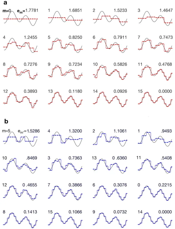
Figure 2-4a shows the reconstructed field with an increasing number of Walsh coefficients (𝑚 ∈ [0, 𝑚𝑚𝑎𝑥]) in sequency ordering. The reconstruction error decreases monotonically as the number of coefficients increases. If the dynamics of the field is known, the Walsh coefficients can be precomputed and sorted so to allocate the avail-able resources to sample the largest coefficients, which provide the most information about the field. Figure 2-4b shows that not only the accuracy of the reconstruction improves monotonically, but also only the first few coefficients are needed to achieve an accurate estimate of the field.

The set of Walsh sequences contains some known set of digital decoupling se-quences such as the Carr-Purcell-Meiboom-Gill (CPMG) sese-quences (𝑤2𝑛, 𝑛 ≥ 1) and

0 1 2 4 8 16 -0.2 -0.1 0 0.1 0.2 ˆ f(m ) 0.2 0.0 0.4 0.6 0.8 1.0 -0.4 -0.2 0.2 0.0 0.4 0.2 0.4 0.6 0.8 1.0 -0.4 -0.2 0.2 0.0 0.4 0.0 0.2 0.4 0.6 0.8 1.0 -0.4 -0.2 0.2 0.0 0.4 0.0 0 1 2 4 8 16 -0.2 -0.1 0 0.1 0.2 PDD CPMG d e f c f(t) f(t) f(t) t (μs) t (μs) t (μs) CPMG PDD CPMG+PDD Sorted sequency, m b 0 1 2 4 8 16 -0.2 -0.1 0 0.1 0.2 Sequency, m ˆ f(m ) a Sequency, m ˆ f(m )

Figure 2-3: Simulate the reconstruction of bichromatic fields with Walsh sequences. Simulated Walsh spectrum for a bichromatic field. Walsh coefficients are presented in a, sequency ordering and b, sorted ordering with decreasing mag-nitude. If the temporal profile of the field is known, the resources can be allocated to extract the most significant information about the field by sampling the largest Walsh coefficients. c, Walsh spectrum up to fifth order (𝑁 = 24 _{= 16)}. The blue dots and red squares respectively indicate the subset of coefficients associated with the PDD sequences (𝑤2𝑛₋₁) and CPMG sequences (𝑤₂𝑛). The field reconstructed

with the first 16 CPMG coefficients (d,), 16 PDD coefficients (e,) and both PDD and CPMG coefficients (f,), remains inaccurate in comparison with the reconstructed field obtained with the first 16 Walsh coefficients (black solid line in d-f).

the periodic dynamical decoupling (PDD) sequences (𝑤2𝑛₋₁, 𝑛 ≥ 1), which have

been studied in the context of dynamical error suppression and noise spectrum recon-struction. Although the CPMG and PDD sequences can be shown to contain some significant information about the field, they do not contain all the significant

infor-15 0.0000 14 0.0926 13 0.1180 12 0.3893 11 0.4768 10 0.5826 9 0.7234 8 0.7276 7 0.7473 6 0.7911 5 0.8250 4 1.2455 3 1.4647 2 1.5233 1 1.6851 1.7781 e m= m=0 14 0.0000 9 0.0732 15 0.1066 8 0.1413 0 0.2215 6 0.3076 7 0.3866 0 .4655 .5408 0 .6360 3 0.7363 .8469 1 .9493 2 1.1061 4 1.3200 1.5286 e m’= m=5 11 13 10 12

a

b

Figure 2-4: Quantify the accuracy of the Walsh reconstruction method. a. Reconstruction of a bichromatic field with an increasing number of Walsh coefficients { ˆ𝑓 (𝑚)_}𝑚𝑚𝑎𝑥

𝑚=0 in sequency ordering. b. Reconstruction of a bichromatic field with an increasing number of Walsh coefficients { ˆ𝑓 (𝑚)_}𝑚′𝑚𝑎𝑥

𝑚=0 sorted by the coefficient magni-tude. A finite number of coefficients is needed to reconstruct an accurate estimate of the field. The upper left and upper right numbers respectively correspond to 𝑚 (in the sequence order) and the 𝑙2-reconstruction error up to the 𝑚′ reconstruction, 𝑒𝑚′.

mation. The CPMG and PDD sequences are indeed symmetric and anti-symmetric functions about their midpoint; they only sample the even and odd symmetries of the field. Figure 2-3c-f shows that the Walsh reconstruction method outperforms the CPMG and PDD sequences, even if the same amount of resources is allocated to sam-ple an equal number of coefficients; because the field does not have a definite parity, the CPMG and PDD sequences fail to accurately reconstruct the field. In addition, these sequences require an exponentially large number of control pulses, which may be detrimental in the presence of pulse errors. Therefore, sampling the field with only these sequences provides incomplete information about the Walsh spectrum and thus leads to inaccurate reconstruction in the time domain.

CPMG and PDD have been used as filters in the frequency domain to achieve frequency-selective detection and reconstruction of noise spectral density.Even for this task, Walsh reconstruction can provide an advantage. Indeed, in the frequency domain, digital filters are trigonometric functions that are not perfectly approximated by delta functions and exhibit spectral leakage, i.e., the non-zero side-lobes of the filter function capture non-negligible signal contributions about other frequencies than the main lobe. Although the CPMG and PDD sequences can be tuned to sample the field at a specific central frequency, they also capture signal at other frequencies, which prevents the accurate reconstruction of time-varying fields. The Walsh reconstruction method removes the need for functional approximations or deconvolution algorithms by choosing the representation that is natural for digital filters: the Walsh basis.

2.2 Demonstrate the Walsh reconstruction method

experimentally with a single nitrogen-vacancy

cen-ter in diamond

We experimentally demonstrate the Walsh reconstruction method by measuring in-creasingly complex time-varying magnetic fields with the electron spin associated with a single nitrogen-vacancy center in diamond in an isotopically purified diamond sam-ple. A single NV center is optically initialized and read out by confocal microscopy under ambient conditions. A coplanar waveguide delivers both resonant microwave pulses and off-resonant time-varying magnetic fields produced by an arbitrary wave-form generator.

2.2.1 Reconstruct the temporal profile of sinusoidal fields

We first reconstructed monochromatic sinusoidal fields, 𝑏(𝑡) = 𝑏 sin (2𝜋𝜈𝑡 + 𝛼), by measuring the Walsh spectrum up to fourth order (𝑁 = 24_{). Figure 2-5b shows the} measured non-zero Walsh coefficients of the Walsh spectrum. As shown in Fig. 2-5c, the 16-point reconstructed fields are in good agreement with the expected fields. We note that, contrary to other methods previously used for a.c. magnetometry, the Walsh reconstruction method is phase selective, as it discriminates between time-varying fields with the same frequency but different phase.

The 𝑚-th Walsh coefficient ˆ𝑓 (𝑚)of the normalized field 𝑓(𝑡) = 𝑏(𝑡)/𝑏 was obtained by sweeping the amplitude of the field and measuring the slope of the signal 𝑆𝑚(𝑏) = sin (𝛾𝑏 ˆ𝑓 (𝑚)𝑇 ) at the origin (Fig. 2-5a). The qubit sensor is first initialized to its ground state |0⟩ and then brought into a superposition of its eigenstates (|0⟩+|1⟩)/√2 by applying a 𝜋

2-pulse along the 𝜎𝑥 rotation axis. During the free evolution time 𝑇 , the qubit acquires a phase difference 𝜑(𝑇 ) = 𝛾 ∫︀𝑇

0 𝑏(𝑡)𝑑𝑡, where 𝛾 is the strength of the interaction with the external time-varying field 𝑏(𝑡) directed along the quantization axis of the qubit sensor. Under a control sequence of 𝑚 𝜋-pulses applied at the zero-crossings of the 𝑚-th Walsh function 𝑤𝑚(𝑡/𝑇 ), the phase difference acquired

−2 −1 0 1 2 −1.0 0.0 1.0 a m=10 m=14 m=6 m=2 3 0 7 11 15 −0.3 0.0 0.3 b Sequency number, m 0 2 4 6 8 10 −1.0 0.0 1.0 c Normalized field, f(t ) f(t)=sin(2πνt) f(t)=cos(2πνt) Evolution time, t (μs) Magnetic field, b (μT) Signal, S m (b) [a.u.] Walsh spectrum, f(m) ^

Figure 2-5: Reconstruct sinusoidal fields with Walsh sequences. a, Measured signal 𝑆𝑚(𝑏) = sin(𝛾𝑒𝑏 ˆ𝑓 (𝑚)𝑇 ) as a function of the amplitude of a cosine magnetic field for different Walsh sequences with 𝑚 𝜋-pulses. Here 𝛾𝑒 = 2𝜋· 28 Hz · nT−1 is the gyromagnetic ratio of the NV electronic spin. The 𝑚-th Walsh coefficient ˆ𝑓 (𝑚) is proportional to the slope of 𝑆𝑚(𝑏) at the origin. b, Measured Walsh spectrum up to fourth order (𝑁 = 24) of sine and cosine magnetic fields 𝑏(𝑡) = 𝑏 sin (2𝜋𝜈𝑡 + 𝛼) with frequency 𝜈 = 100 kHz and phases 𝛼 ∈ {0, 𝜋/2} over an acquisition period 𝑇 = 1/𝜈 = 10 𝜇s. Error bars correspond to 95 % confidence intervals on the Walsh coefficients associated with the fit of the measured signal. c, The reconstructed fields (filled squares) are 16-point piecewise-constant approximations to the expected fields (solid lines, not a fit). Error bars correspond to the amplitude uncertainty of the reconstructed field obtained by propagation of the errors on the estimates of the uncorrelated Walsh coefficients.

after an acquisition period 𝑇 is 𝜑𝑚(𝑇 ) = 𝛾 ∫︀𝑇

0 𝑏(𝑡)𝑤𝑚(𝑡/𝑇 )𝑑𝑡 = 𝛾ˆ𝑏(𝑚)𝑇, which is proportional to the 𝑚-th Walsh coefficient of 𝑏(𝑡). A final 𝜋

2-pulse applied along the 𝜎𝜃 = cos (𝜃)𝜎𝑥+sin (𝜃)𝜎𝑦 rotation axis converts the phase difference into a measurable fluorescence signal 𝑆𝑥𝜃. -1 0 1 12 13 14 15 16 17 a F lu o re sce n ce (kcp s) Field amplitude, |Φ| (Vpp) -1 0 1 0 0.5 1 b Field amplitude, |Φ| (Vpp) N o rma lize d si g n a l -2 0 2 -1 0 1 c Field amplitude, b (μT) Ave ra g e d si g n a l

Figure 2-6: Extract the Walsh coefficient from the fluorescence signal. Ex-ample of experimental data for measuring the 𝑚-th Walsh coefficient. a, Measured fluorescence signals 𝑆𝑥𝑦 and 𝑆𝑥¯𝑦 for a sinusoidal field measured with the 𝑚 = 1 Walsh sequence. b, The measured fluorescence signals are normalized with respect to the reference signals. c, Average normalized fluorescence signal 𝑆𝑚(𝑏) whose slope at the origin is proportional to the 𝑚-th Walsh coefficient ˆ𝑓 (𝑚)of the normalized field 𝑓(𝑡).

Although performing a single measurement with 𝜃 = 𝜋/2 is enough to extract the 𝑚-th Walsh coefficient, we sweep the field amplitude of 𝑏(𝑡) = 𝑏 𝑓(𝑡) to better estimate it (Fig. 2-6). The 𝑚-th Walsh coefficient ˆ𝑓 (𝑚) of the normalized field is obtained from the slope at the origin of the normalized fluorescence signal averaged over 𝑀 ∼ 105 _{measurements: 𝑆} 𝑚(𝑏) = sin (𝛾𝑒𝑏 ˆ𝑓𝑚𝑇 ) = 𝑆𝑥 ¯𝑦−𝑆𝑥𝑦 𝑆𝑥 ¯𝑦+𝑆𝑥𝑦 · 𝑆0+𝑆1 𝑆0−𝑆1, where 𝑆0 is

the fluorescence count rate of the 𝑚𝑠 = 0 state measured after optical polarization, and 𝑆1 is the fluorescence count rate of the 𝑚𝑠 = 1 state measured after adiabatic inversion of the qubit with a 600 ns frequency-modulated chirp pulse over a 250 MHz frequency range centered around the resonance frequency.

In practical applications for which the amplitude of the field cannot be swept, the 𝑚-th Walsh coefficient can be equivalently measured by sweeping the phase 𝜃 of the last read-out 𝜋

2-pulse and fitting the normalized signal to a cosine function: 1_{− 2𝑆}𝑚(𝜃) = cos (𝛾𝑒ˆ𝑏𝑚𝑇 − 𝜃) = 𝑆_𝑆𝑥𝜃_1−𝑆−𝑆₀0. This procedure gives an absolute estimate of ˆ_{𝑏(𝑚) rather than an estimate of the normalized coefficient ˆ𝑓 (𝑚) = ˆ𝑏(𝑚)/𝑏.}

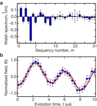
7 0 15 23 31 −0.3 −0.2 −0.1 0.0 0.1 0 2 4 6 8 10 −1.0 0.0 1.0 Walsh spectrum, f(m) ^ Norm alized field, f(t ) a Sequency number, m b Evolution time, t (μs)

Figure 2-7: Reconstruct bichromatic fields with Walsh sequences. a, Mea-sured Walsh spectrum up to fifth order (𝑁 = 25) of a bichromatic magnetic field 𝑏(𝑡) = 𝑏 _{· [𝑎}1sin (2𝜋𝜈1𝑡 + 𝛼1) + 𝑎2sin (2𝜋𝜈2𝑡 + 𝛼2)] with 𝑎1 = 3/10, 𝑎2 = 1/5, 𝜈1 = 100 kHz, 𝜈2 = 250 kHz, 𝛼1 = −0.0741, and 𝛼2 = −1.9686. The zero-th Walsh coefficient ˆ𝑓 (0) corresponds to a static field offset that was neglected. b, The reconstructed field (filled squares) is a 32-point approximation to the expected field (solid line, not a fit). Error bars correspond to the amplitude uncertainty of the reconstructed field obtained by propagation of the errors on the estimates of the uncorrelated Walsh coefficients.

2.2.2 Reconstruct the temporal profile of bichromatic fields

We further reconstructed a bichromatic field 𝑏(𝑡) = 𝑏 [𝑎1sin (2𝜋𝜈1𝑡 + 𝛼1)+𝑎2sin (2𝜋𝜈2𝑡 + 𝛼2)]. Figure 2-7a shows the measured Walsh spectrum up to fifth order (𝑁 =25_{). As shown}

in Fig. 2-7b, the 32-point reconstructed field agrees with the expected field, which demonstrates the accuracy of the Walsh reconstruction method (Fig. 2-4). In con-trast, sampling the field with an incomplete set of digital filters, such as the CPMG and PDD sequences, extracts only partial information about the dynamics of the field (Fig. 2-3). By linearity of the Walsh transform, the Walsh reconstruction method applies to any polychromatic field (and by extension to any time-varying field), whose frequency spectrum lies in the acquisition bandwidth [1/𝑇, 1/𝜏] set by the coherence time 𝑇 ≤ 𝑇2 and the maximum sampling time 𝜏 = 𝑇/𝑁, which is in turn limited by

the finite duration of the control 𝜋-pulses.

2.2.3 Reconstruct the temporal profile of arbitrary time-varying

fields

Figure 2-8: Characterize the transmission properties of the coplanar waveg-uide. The conversion factor converts the amplitude of the electric field Φ(𝑡) into the amplitude of the magnetic field 𝑏(𝑡) measured by the NV center. The conver-sion factor depends linearly on the frequency. Error bars are standard deviation of measurements.

As a proof-of-principle implementation, we measured the magnetic field radi-ated by a physical model of a neuron undergoing an action potential Φ(𝑡) approxi-mated by a skew normal impulse [45, 46, 47]. Due to its linear response in the kHz regime (Fig. 2-8), our coplanar waveguide acts as the physical model of a neuron, with the radiated magnetic field given by the derivative of the electric field [48, 49]: 𝑏(𝑡) = 𝑑Φ(𝑡)/𝑑𝑡 (Fig. 2-9).

Calibrate the transmission spectrum of the coplanar waveguide

Coplanar waveguides were fabricated by e-beam photolithography on microscope glass coverslips, soldered on a PCB board, and mounted to the confocal microscope. Elec-tric waveforms Φ(𝑡) (Vpp) were generated with an arbitrary waveform generator, amplified, and sent through the coplanar waveguide. The coplanar waveguide radi-ates a magnetic field 𝑏(𝑡) (nT) at the location of the NV center which can be derived from Φ(𝑡) via a conversion factor 𝑘(𝜈) (nT · Vpp−1

).

with sinusoidal oscillating fields (𝜈 = 1/𝑇 ) sampled with the corresponding Walsh sequence 𝑤𝑚(𝑡/𝑇 ). The amplitude of the field was swept and the normalized Walsh coefficient was extracted from the measured signal 𝑆𝑚(𝑏) = sin (𝛾𝑒𝑏 ˆ𝑓 (𝑚)𝑇 ). The slope at the origin 𝜇𝑉 𝑝𝑝 = 𝛾𝑒𝑓 (𝑚)𝑇ˆ was compared with the value computed analytically, e.g., by choosing ˆ𝑓 (1) = 2/𝜋for the spin-echo sequence (m=1). The conversion factor 𝑘 = 𝜇𝑛𝑇/𝜇𝑉 𝑝𝑝 (nT · Vpp−1) was calculated from the ratio between 𝜇𝑛𝑇 calculated analytically and 𝜇𝑉 𝑝𝑝 measured experimentally at different frequencies.

As shown in Fig. 2-8, the conversion factor 𝑘(𝜈) increases linearly in the frequency range of interest. Taking into account the intrinsic 90∘ _{phase shift between the electric} and magnetic fields, we have 𝑏(𝜈) = −𝑖𝑐𝜈Φ(𝜈) such that 𝑏(𝑡) = −𝑐𝑑Φ(𝑡)

𝑑𝑡 with 𝑐 = 25.4 𝜇T · (Vpp · kHz)−1. Therefore, our coplanar waveguide behaves as the physical model of a neuron, with the magnetic field given by the first derivative of the electric field.

Simulate the magnetic field radiated by a single neuron

The creation and conduction of action potentials is the primary communication mean of the nervous system. The flow of ions across neuronal membranes produce an electric field that propagates through the axon of single neurons. The electric signals carried by the action potentials radiate a magnetic field given approximately by the first derivative of the action potential [48, 49]. As shown in Fig. 2-9, we approximated the action potential by a skew normal impulse and extracted the physical parameters by fitting the simulation data obtained for a rat hippocampal mossy fiber boutons [46]. The action potential was rescaled to perform proof-of-principle measurements.

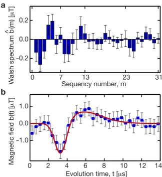
Reconstruct the simulated magnetic field radiated by a single neuron The Walsh coefficients were measured by fixing the amplitude of the field and sweep-ing the phase of the last read-out pulse to reconstruct the absolute field 𝑏(𝑡) rather than the normalized field 𝑓(𝑡). This protocol is in general applicable when the field amplitude is not under experimental control. Figure 2-10a shows the measured Walsh spectrum up to fifth order (𝑁 = 25_{). As shown in Fig. 2-10b, the 32-point}

recon-0 0.25 0.5 0.75 1.0 1.25 1.5 1.75 2.0 -100 -5 0 0 50 t (ms) Φ (t ) (mV) Action potential Skew normal distribution fit 0 2 4 6 8 10 12 14 -0.5 0.0 0.5 t (μs) Φ (t ) (V p p ) 0 2 4 6 8 10 12 14 -2.0 -1.0 0.0 1.0 t (μs) b (t ) (μ T ) a b

Figure 2-9: Simulate an action potential. a ,The simulated action potential of a rat hippocampal mossy fiber boutons [46] is approximated by a skew normal impulse. b, The action potential is rescaled to perform the Walsh reconstruction experiment, with the radiated magnetic field corresponding to the first derivative of the action potential.

structed field is in good agreement with the expected field. Although neuronal fields are typically much smaller than in our proof-of-principle experiment with a single NV center, they could be measured with shallow-implanted single NVs [50, 51, 52, 53] or small ensembles of NV centers [10, 44, 54].

The total measurement time for acquiring all the data of the 𝑇 = 14 𝜇s waveform presented in Fig. 2-10, excluding dead times associated with computer processing and interfacing, was less than 4 h. Each of the 𝑁 = 32 Walsh coefficients were obtained from two 𝑀′ _{= 90measurements of the fluorescence signal as a function of the phase} and conjugate phase of the last readout pulse to correct for common-mode noise (we note that in a well-calibrated, temperature stabilized and isolated setup this step is unnecessary). Each experimental point was averaged over 𝑀 = 105 _repetitive measurements due to low light-collection efficiency. The length of each sequence was about 42 𝜇s, including the two waveform measurements (28 𝜇s), optical polarization and readout periods (5 𝜇s), adiabatic inversion (4 𝜇s) used for calibration purposes but not necessary, and waiting time (5 𝜇s).

0 7 13 23 31 −0.2 0.0 0.2 0 2 4 6 8 10 12 14 −1.0 0.0 1.0 Walsh spectrum b (m) [ μ T] ^ Mag n et ic f ie ld b (t ) [ μ T] a Sequency number, m b Evolution time, t [μs]

Figure 2-10: Reconstruct arbitrary time-varying fields with Walsh se-quences. a, Measured Walsh spectrum up to fifth order (𝑁 = 25_{) of the} mag-netic field radiated by a skew normal impulse flowing through the physical model of a neuron. The Walsh coefficients were obtained by fixing the amplitude of the field and sweeping the phase of the last read-out 𝜋/2-pulse. The acquisition time for measuring all the Walsh coefficients was less than 4 hours. Error bars correspond to 95 %confidence intervals on the Walsh coefficients associated with the fit of the mea-sured signal. b, The reconstructed field (filled squares) is a 32-point approximation to the expected field (solid line, not a fit). Error bars correspond to the amplitude uncertainty of the reconstructed field obtained by propagation of the errors on the estimates of the uncorrelated Walsh coefficients.