Collisionless ion collection by a sphere in a weakly magnetized plasma

Collisionless Ion Collection by a Sphere in a

Weakly Magnetized Plasma

by

Leonardo Patacchini

Ingenieur dipl6me de l'Ecole Polytechnique (X2002)

Submitted to the Department of Nuclear Science and Engineering

in partial fulfillment of the requirements for the degree of

Master of Science in Nuclear Science and Engineering

at the

MASSACHUSETTS INSTITUTE OF TECHNOLOGY

@

Massachusetts I

Author ...

May 2007

yo Vt. c7o -7lJ

nstitute of Technology

Department of Nuclde

2007. All rights reserved.

ar Science and Engineering

May 17, 2007

Certified by...

..

Ian H. Hutchinson

Professor

Thesis Supervisor

Certified by

Brian Labombard

S

A P9iipal Research Scientist

,

Thesis Reader

Accepted

by...

MASSACHUSETTS INSTmTUTE-OF TECHNOLOGY

OCT

12

2007

ARCHIVES

LIBRARIES

x.i,

Jeffrey A. Coderre

Chairman, Graduate Committee

Collisionless Ion Collection by a Sphere in a Weakly

Magnetized Plasma

by

Leonardo Patacchini

Submitted to the Department of Nuclear Science and Engineering on May 17, 2007, in partial fulfillment of the

requirements for the degree of

Master of Science in Nuclear Science and Engineering

Abstract

The interaction between a probe and a plasma has been studied since the 1920s and the pioneering work of Mott-Smith and Langmuir [1], and is still today an active topic of experimental and theoretical research. Indeed an understanding of the current collection process by an electrode is relevant to diverse matters such as Langmuir and

Mach-probes calibrations, dusty plasma physics, or spacecraft charging.

Recent simulations relying on the ad hoc designed code SCEPTIC have fully addressed the collisionless and unmagnetized problem for a drifting collector idealized as a sphere. SCEPTIC is a 2d/3v hybrid Particle In Cell (PIC) code, in which the ion motion is fully resolved, while the electrons are treated as a Boltzmann distributed fluid [2, 3]. In the present work we tackle the transition between the unmagnetized and the weakly magnetized regime of ion collection by a spherical probe (The mean ion Larmor radius rL > r,) in a collisionless plasma (The ion mean free path Am,fp > rp).

When the sphere is at space potential, we demonstrate that the ion current depen-dence on the background magnetic field B is linear for low B, and provide analytical expressions for this dependence.

When the probe potential can not be neglected, the problem shows two distinct scale lengths: A collisionless layer of a few rp close to the probe, followed by a collisional presheath of a few AXmfp. The chosen approach is to resolve the collisionless scale-length with SCEPTIC, while using appropriate outer boundary conditions on the potential and ion distribution function to connect with the unresolved collisional presheath. We present results of our numerical simulations for a wide range of plasma parameters of direct relevance to Langmuir and Mach-probes.

Thesis Supervisor: Ian H. Hutchinson Title: Professor

Thesis Reader: Brian Labombard Title: Principal Research Scientist

Acknowledgments

The first lines of this thesis should be words of gratitude to those who contributed to this work.

First of all I would like to thank my advisor Pr. Hutchinson. In addition to his physical insight and contagious interest for Mach-probes, I shall not forget his uninterrupted support and time-commitment. I acknowledge that his tens of papers and thesis drafts proofreadings could have been fatal to many English Professors.

I express my sincere gratitude to the MIT Nuclear Science and Engineering De-partment as well as to the US DeDe-partment of Energy, whose funding made this thesis possible.

I would also like to thank Pr. Giovanni Lapenta, who hosted me in his research group at Los Alamos National Laboratory during the summer 2006. This period resulted in a fruitful collaboration, and helped me mature my knowledge on topics of direct relevance to this thesis.

I am deeply indebted to my parents for their love and support throughout my entire life, and for their encouragement to undertake my Doctoral research in the United States.

I dedicate this thesis to Jean Marie Benad. His devotion to the teaching of physics despite the misfortunes of life have always aroused the deepest; respect and admiration in me. Oii que vous soyez, j'espire que vous conscientisez tout ce que vous avez apporte a vos eleves.

Contents

I Analytical basis 19

1.1 Position of the problem ... 19

1.2 Basic plasma properties ... 21

1.2.1 Infinite uniform plasmas . . . . 21

1.2.2 Analytical current calculations . . . . 23

1.3 Free flight ion current to a spherical probe . . . . 25

1.3.1 Unmagnetized plasma ... 25

1.3.2 Magnetized plasma with Vd

IIB

. . . . 26

1.4 Basic charging mechanisms with non negligible electric fields . . . . . 31

1.4.1 Electron density ... 31

1.4.2 Orbital Motion Limited ion current in an unmagnetized plasma 32 1.4.3 Canonical upper-bound in a stationary, magnetized plasma . . 33

1.5 Coupling of Vlasov and Poisson equation . . . . 35

1.5.1 Debye shielding in a spherical well . . . . 35

1.5.2 Anti-shielding in a one-dimensional well . . . . 37

1.5.3 The Bohm Criterion ... 40

1.5.4 Helical upper bound and adiabatic limit currents . . . . 42

1.5.5 Quasicollisionless collection in a strongly magnetized plasma . 45 II Solving the problem with the PIC code SCEPTIC 49 II.1 SCEPTIC Overview ... ... 49

II.1.1 The unit system . . . . 49

II.1.3 The Geometry ...

11.2 Development of a parallelized Poisson solver . . . . II.2.1 Successive Over Relaxation . . . .

II.2.2 Parallel code structure . . . . II.2.3 Performance expectation . . . . II.2.4 Optimization ... .. ...

II.2.5 Test ... .. .. ...

II.3 Development of a symplectic magnetized particle mover

II.3.1 Motivation... ...

II.3.2 Single particle Hamiltonian . . . .

II.3.3 Practical implementation . . . . II.3.4 Benchmarking against direct orbit integration . II.4 The boundary conditions ...

II.4.1 Conditions on the potential . . . . II.4.2 Particle reinjection ...

III Solutions for a stationary plasma

III.1 Weakly-focusing and Strongly-focusing regimes . . . . III.2 Space-charge distribution ... ...

III.2.1 Quasineutral plasma . . . . III.2.2 Plasma with finite shielding . . . .. III.3 Total ion current to the probe . . . .

III.3.1 Dependence on 3 ... . . . ... III.3.2 Dependence on ADe .. ...

III.3.3 Dependence on Xp ... ...

III.4 Angular distribution of the ion current . . . . III.4.1 Quasineutral regime ...

III.4.2 Plasma with finite shielding . . . . IV Solutions for a flowing plasma

IV.1 Cold ion orbits in a flowing plasma . . . .

. . . . 51 . . . . . . 52 . . . . . . 52 . . . . . . 53 . . . . . . 53 . . . . 55 . . . . 55 . . . . . . 57 . . . . 57 . . . . . . 58 . . . . . . 59 . . . . . . 61 . . . . 62 . . . . . . 62 . . . . 64 67 67 68 68 70 76 76 77 79 82 82 83 85 85

IV.2 Space-charge distribution ... IV.2.1 Quasineutral regime ...

IV.2.2 Plasma with finite shielding . . . . IV.3 Total collected current ...

IV.4 Angular distribution of the ion current for weakly focusing probes . .

IV.4.1 Quasineutral regime . . . . IV.4.2 Plasma with finite shielding and equithermal ions and electrons IV.5 Flux asymmetry reversal suppression for strongly focusing probes . .

V Conclusions

V.1 Review of our computation hypothesis . . . . V.2 Implications of our results ...

V.3 Suggestions for future work ...

91 91 94 97 98 98 102 106 111 111 112 113

A Low 3 expansion of Whipple-like integrals 115

A.1 Sphere at space potential in a drifting plasma . . . . 115

A.1.1 Current drawn from orbits in the magnetic shadow: t' . . . . 116

A.1.2 Current drawn from the other orbits: tout . . . ..116

A.1.3 Analysisof t*(s,t,u) ... 117

A.1.4 Analysis of tUt ... 119

A.1.5 Analysis of t..' ... 120

A.1.6 Conclusion . . . . . 121

A.2 Charged sphere in a stationary plasma: Upper bound . . . . 122

A.2.1 Current drawn from the orbits in the magnetic shadow: tn . . 123

A.2.2 Current drawn from the other orbits: tot . . . ..123

A.2.3 Analysisof Lp ... 123

A.2.4 Analysis of tup ... 124

A.2.5 Conclusion. .. . . . ... . . . . ... . . . . .. . 125

A.3 Charged sphere in a stationary plasma: Lower bound . . . . 125

A.3.1 Current drawn from the orbits in the magnetic shadow: Low . 125 A.3.2 Analysisof oin...126

A.3.3 Analysis of t ... ... . ... 126 A.3.4 Conclusion ... . . .. .. ... ... 126

B Derivation of the OML currents to a sphere and infinite cylinder 127

B .1 Sphere . . . . . . . . .. 127

B.2 Infinite cylinder ... . . ... 129

List of Figures

I-1 Spherical and cylindrical coordinates of the problem . . . .. I-2 Collection orbits in the presence of a background magnetic field . I-3 Magnetized orbits parameterization . . . .. I-4 Ion current to a stationary spherical probe at space potential . . .

I-5 Ion current to a drifting spherical probe at space potential ... I-6 Ion and electron densities in a one-dimensional well ... I-7 Bohm criterion in a half one-dimensional well ...

I-8 Helical upper bound as a function of

3

...

I-9 Models of ion distribution function in a one-dimensional presheath

II-1 II-2 II-3 II-4 II-5 II-6 II-7 III-1 III-2 III-3 III-4 III-5

Spherical mesh used in SCEPTIC . . . . Principle of a SOR block-solver . . . .

Block-solver performance test . . . . Schematic of the subcycling algorithm . . . . Cyclotronic integrator benchmark . . . . SCEPTIC physical domain . . . . Models of differential fluxes for ion reinjection . . . . Orbit interpretation of the probe focusing properties . . . .

Charge-density profiles dependence on 0 for ADe = 0 . . . .

Charge-density contour plot evolution with 3 for ADe = 0 . Charge-density contour plot evolution with Ti for ADe = 0 .

Charge-density profiles dependence on

f

for ADe : 0 . . . .

III-6 Charge-density contour plot evolution with ADe for 3 = 1 and Ti = 0.1 74

. . . . 51 . . . . 54 . . . . 56 . . . . 60 . . . . 61 . . . . 63 .... 65 . . . . 68 . . . . 69 . . . . 71 . . . . 72 . . . . 73

III-7 Potential contour plot evolution with ADe for = 1 and Ti = 0.1

-III-8 Ion current as a function of j for ADe 6 0

Ion current as a function of 3 for AD6

7

0 Ion current as a function of3 for ADe ) 0

Ion current as a function of for ADe 7/ 0

Variation of the slope factor C, with AD6

Ion current dependence on ADe . . . . . .

Ion current dependence on Xp ...

Angular dependence of the ion current for Magnetic field induced asymmetry for AD, Angular dependence of the ion current for

and = and = and = III-9 III-10 III-11 III-12 III-13 III-14 III-15 III-16 III-17 IV-1 IV-2 IV-3 IV-4 IV-5 IV-6 IV-7 IV-8 IV-9 IV- 10 IV-11 IV-12 IV-13 IV-14 IV-15 IV-16 IV-17 IV-18 . . . . . 76 1.0 . . . . 77 0.3 . . . . 78 0.1 . . . . 78 . . . . . 79 . . . . . 80 ... ₈₁ . . . . . 82 . . . . . 83 . . . . . 84

Orbit interpretation of the fux asymmetry reversal . . . . Evolution of the depletion cone with . . . . Evolution of the depletion cone with ADe . . . . . Charge-density profiles on axis for ADe = 0 . . . . . Magnetic field effect on Mach-cone shaped rarefactions . . . Evolution of the ion density distribution with 0 for ADe )/ 0 Evolution of the potential distribution with

/

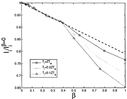
for ADe z 0 . . Wake in the supersonic, magnetized regime . . . . Ion current dependence on 3 for ADe - 1 and T = 1 ... Ion current dependence on

/3

for AD, =1 and Tj = 0.1 . . . . Angular dependence of the ion current for AD = 0 . . . . . . Mach-probe calibration factor for ADe = 0 and Ti 1 . . . . Angular distribution of the ion current for Tj = 1.0 and ADe Angular distribution of the ion current for Tj = 1.0 and AD =1 =0 . . . 86 . . . 87 S 88 .. 91 . . . 93 .. 95 . . 96 . . . 97 . . 98 .. 99 .. 100 . .. 102 .0 . 103 .1 . 104 Mach-probe calibration factor contour lines for ADe 0 and T = 1 .

Mach-probe calibration factor for AD6

7

0 and T = 1 . . . ..

Flux asymmetry reversal suppression by B at Ti = 0.1 . . . . Mach-probe calibration factor for ADe = 1.0 and Ti = 0.1 . . . .

105 106 107 108 ADe - 0 =- 0 NDC )4 0

IV-19 Flux asymmetry reversal suppression by B at Tj = 0.01 . . . . 109

B-1 OML current calculation: Sphere . . . . 128 B-2 OML current calculation: Infinite cylinder . . . . 130 B-3 Comparison of the spherical and cylindrical probes OML current . . 132

List of Tables

II.1 Fundamental units used with SCEPTIC . . . . 49

Nomenclature

rp Probe radius

Ti,e Ion (Electron) temperature

Vti,e Ion (Electron) thermal speed

Z Ion charge

cs Sound speed (Ion acoustic waves)

'Y Ratio of specific heats for the ion species

n., Electron density at infinity IF _{Ion thermal charge flux density}

I? Ion thermal current to the probe

ADi,C Ion (Electron) Debye length A, Plasma shielding length

B Magnetic field

Q Larmor angular frequency rL Ion mean Larmor radius

Probe radius over the Ion mean Larmor radius

f,

Ion (Electron) distribution function at infinity

Vd Ion drift velocity

V Electrostatic potential

Electrostatic potential normalized to Te

X Electrostatic potential normalized to -pV Probe potential

Chapter I

Analytical basis

1.1

Position of the problem

Since the early days of laboratory plasmas scientists have been interested in studying the behavior of bodies inserted in gas discharges. The pioneering work of Mott-Smith and Langmuir on the matter [1] was mainly motivated by the prospect of diagnosing the ions and electrons distribution functions in a plasma by measuring their current to a conducting wire, or Langmuir probe. Because we have today a good understanding of particle-flux sensing devices in several regimes of operation, such probes are still widely used in modern plasma diagnostics [4].

The theory of current collection in a plasma would not have aroused much in-terest outside the community of experimentalists if its applications were limited to diagnostic purposes. Fortunately dust particles in natural or artificial plasmas, as well as man-made satellites, obey the same physics of Langmuir probes. Unless oth-erwise indicated, the term "probe" will be used regardless of the physical nature of the collector.

An ideal probe absorbs every ion and electron striking it. In steady state, it will release neutral atoms and/or molecules at a rate that balances the incoming flux of ions, which has been neutralized by the incoming electrons or the electrons supplied by an external bias circuit. The deviations from ideality come from different Solid state physics reactions resulting in electron emission at the surface, whose relative

importance depends upon the experimental conditions. Usually the most relevant effects are Photoemission, Secondary emission, and Thermionic emission. A quanti-tative treatment showing how those phenomena can strongly influence the charging of dust particles has been performed by Delzanno and Bruno [5]. In some cases ion-induced secondary emission is present as well. Although the conditions for a probe to behave as ideal are rarely met in practice, we will work under the assumption that those conditions are fulfilled, and hence shall only be concerned by the current drawn from the bulk plasma. We also assume that the charge-exchange mean-free-path is much longer than the probe size, in order to neglect the interaction between the neutrals released by the probe and the incoming ions.

The electrostatic potential of Langmuir probes is artificially biased with respect to the surrounding plasma, usually negatively. Ideal floating probes (i.e. non connected to an external circuit) tend to charge negatively as well due to the high electron mobility [4]. In either case, relating the current to the plasma properties requires an understanding of how the probe potential locally perturbs the plasma, and hence the particle distributions. This interaction between the plasma and the collector is governed by basic Plasma physics, that we will study under the assumption that the probe can be idealized as a sphere. The geometry under consideration is illustrated

in Fig. (I-1).

is

Figure I-1: Spherical and cylindrical coordinates of the problem. The magnetic axis (External B-field) defines the z-direction.

The unmagnetized problem (that is to say without background magnetic field) has been solved by Hutchinson [2, 3] in the limit of zero collisionality by means of the Particle in Cell (PIC) code SCEPTIC. The opposite limit of a strongly magnetized plasma (3 > 1, where 3 is the probe radius divided by the mean ion Larmor radius) has been treated by Chung and Hutchinson [6, 7] through one-dimensional fluid and kinetic calculations in a "quasi-collisionless" plasma. In each case the angular distri-bution of ion current has been computed for a wide range of drift velocities and ion to electron temperature ratios.

The intermediate magnetic field regime (/3 - 1) has received non negligible at-tention, be it from an experimental [8] or an analytical [9, 10, 11, 12] point of view. Three dimensional PIC simulations of electron collection by a spherical satellite in a magnetoplasma flowing perpendicular to the magnetic field have been performed as well [14], however the results are rather crude and qualitative.

The main goal of the present thesis is to perform a comprehensive and quantita-tive study of ion collection by a negaquantita-tively charged spherical probe using the code SCEPTIC under the condition of negligible collisionality, and in the presence of a weak magnetic field parallel to the drift velocity. The present Chapter summarizes existing theories necessary to an understanding of SCEPTIC operation and results, and develops new analytical expansions at low

/3

to the current collected by a sphere at space potential. Chapter II gives an overview of the code operation, and of recent modifications necessary to implement the magnetic field. Chapter III presents the numerical results in the flow-free regime, while Chapter IV treats the drifting case.

1.2

Basic plasma properties

1.2.1

Infinite uniform plasmas

The simplest classical plasma is a uniform, infinite, isotropic, fully ionized neutral gas consisting of a single species of ions with mass mi, charge Z and uniform density ni = noo/Z, and electrons with mass me and uniform density ne -nr. Because the

proton-to-electron mass ratio is extremely large (-- = 1836) and thermalization is

driven by Coulomb collisions, it is often the case that ions and electrons equilibrate among themselves much faster than with each other. Therefore the two species can be described by Maxwellian distributions with different temperatures Ti,e and drift

velocities

Vdi,e-If we define the thermal speed of a species by:

vt = (I.1)

the shifted Maxwellian distribution function f'(v), where f"(v)d3v is the number of particles in the velocity range d3v, is given by:

f(v) = t/) exp(- 2Vd ) (I.2) By construction we have: n = ff(v)d3v (I.3) Vd = vf (v)d3v (I.4) 1/'2

T =

f(v- Vd)2fc (v)d v (I.5) (I.6)

vt appears as a measure of the random velocity of the particles, and is related to

their mean kinetic energy by < E, >= ýmv2. The random flux-density is defined as the one-directional charge flux-density in a frame moving with velocity vd, where the

plasma is therefore at rest:

F°= Z f =o(v)vxd3v = Zn 2Vý(.7)

of specific heats along this direction, 7, is given by:

1 dp

()

x -T dnj dy=dz=O0

We can now define the sound speed c, in the ex direction as the speed of ion acoustic waves in the ion reference frame:

ZTe +72Tq

c - T+ T vti (I.9)

In most plasma experiments the electron drift velocity is much smaller than the electron thermal speed (Ivde

<<

Vte), it is therefore appropriate to consider the elec-trons as stationary. This thesis is based on this assumption, and from now on the term "drift velocity" refers to the ion species. The relevant values for the drift velocity range from zero to a few sound speeds.

1.2.2

Analytical current calculations

The theories and computations developed in this thesis, intended to calculate the ion current to a spherical probe, assume the ions and electrons far from the collector, or "at infinity", to be described by the preceding model. Because the probe induces a local perturbation on the electrostatic fields and particle distribution functions, the ion flux density to the probe surface is not simply given by Eq. (I.7) with n = no/Z. Two main approaches can be followed when searching for analytic expressions for the steady-state current effectively collected by the probe, when collisions can be neglected.

Approach 1

The first approach is to use Vlasov's equation, governing the temporal and spatial evolution of the distribution function:

df

_

Of

Ze

dt

_dt

Ofrt - V Zf + -(E +vAB).Vf ₌ 0 (I.10)

Along an orbit, because phase-space density is conserved, -=f 0. If each orbit

dt

-striking the probe can be traced back to infinity, the distribution function at the probe surface is straightforwardly given by:

fprobe (v, x) = f Vo) .11)

where v, is the velocity that a particle striking the probe with position (v, x) had at infinity. If v,, is the component of the velocity normal to the probe surface and directed inwards, the total current collected is:

I

= Z

v~.fprobe

(v,

x)d3

_vd

3_x

_(I.12)

Jpobe

Unfortunately there are two situations where this approach can not be followed: When some orbits intersect the probe more than once, and when it is not possible to find an analytic relationship between (v, x) and voo.

Approach 2

When the preceding path fails, one can consider a control volume Q containing the probe, but whose surface is at an arbitrary location where the distribution function is known, such as infinity. The collected current is:

I =Zf fj

v, f (v)H(v, x)d3vd3

x (1.13)

where OQ is the surface of the control volume over which the integration is performed, v, the velocity component normal to the control surface and directed inwards, and H(v, x) an impact parameter equal to 1 if a particle whose initial position in phase-space is (v, x) is collected, and 0 otherwise.

1.3

Free flight ion current to a spherical probe

1.3.1

Unmagnetized plasma

The free flight model of current collection is a collisionless model where any electric field is neglected. Therefore although we immediately specialize to the ions, this model can equivalently be applied to the electrons. Unmagnetized orbits emerging from a convex probe are therefore straight lines and connect to infinity, hence we can use the first approach described in Section 1.2.2:

F{f = Z f (v)vd 3v (I.14)

The integration has been performed analytically in Ref. [2] in the case of a spherical probe with

f'

given by Eq. (I.2) (See Fig. (I-1) for a description of the coordinate system).

S_{(vcosO) =}

_{Fexp( (}

_{)2 COS2 ) - \/7e-rC}

_(cos

₀₎ vd _{cos 0 (I.15)}

vtL

Vti _{VtV i}

By integrating Eq. (I.15) over the sphere we find the total current:

ffvvd Vli Vdl

I = I - exp(- 2 ) + ( + )erf( ) (I.16)

112 vt2i 2 vtj 2Vd vt

Here and in the rest of the Thesis, = n tis the ion random charge flux density (we recall that the ion density at infinity is n,/Z), and I° _{= 47r•.2? is}

the ion random thermal current collected by the sphere. Similar calculations for an infinite planar probe perpendicular to the plasma drift and collecting particles from both sides (total area of the two faces: A) yield:

If =

1A

[exp(- 2) + V- Vderf( Vd) (I.17)

1.3.2

Magnetized plasma with

Vd

1 B

The picture is more complicated in the presence of a background magnetic field, because as shown in Fig. (I-2) not all the orbits originating from the probe, be it convex, connect to infinity. We must therefore resort to the second approach described in Section 1.2.2.

Magnetic axis

Orbit connected to infinity

/ ' /

ii

\

/ "

\ \ / \

Orbit closed on the sphere

Figure I-2: Schematic representation of the two kind of orbits intersecting the probe. In a collisionless plasma, orbits that close on the sphere are empty.

The current to the probe depends on vt, va, and on the non-dimensional factor

S rp/rL, which is a measure of the magnetic field defined as the ratio of the probe radius over a mean ion gyroradius.

/

3

=

(I.18)

rrTi mi 2Z2e2B2

At/3 = 0, the current is given by Eq. (I.16):

I

=

I

exp(- )

"ti

+

)erf(

)

(I.19)

L2 vti 2 vtj 2Vd vti

2 VUiVt

In the limit

/3

> 1, the particles are tight to the magnetic field lines and the total current is therefore given by Eq. (I.17) with A = 27rr (double of the probe

I [,V VO' + V- d 1d

V11 = I

L0

xp(

2

)

+ "d-erf(U) (1.20)

2 lvU vti vti

In the intermediate magnetic field regime (0 < 03 < 0o), the current to a spher-ical electrode of radius unity at space potential can be evaluated by summing the contribution of helices of radius s, wave length 27rt, guiding center distance to the magnetic axis of the probe u, and phase V e [0 : 27r] distributed according to a drift-ing Maxwellian (Only four variables are necessary to describe the helices because we have poloidal symmetry about the magnetic axis). Fig. (I-3) is a schematic of the problem:

Figure I-3: Schematic of three different kind of orbits. Solid portions of orbits are visible, dashed portions are behind the sphere, and dotted portions are inside the probe. Orbit no1 has si + ul > 1 and isi - ul < 1. The phase 1, is such that the orbit crosses the sphere, but because the wavelength is "long" (t, > t*(sl, ti, ui), see Appendix A), there are phases

4

such that H(ul, sl, ti,

4)

= 0. Orbit n02, for which the geometrical meaning of s, t and u is shown, has s2 + u1 > 1 and

Is8

2 - u21 < I

It is a critical orbit because H(U2, 82, t2, 2) = 1 regardless of V2 (t2 = t2(s 2, t2, u2)).

Orbit n03 has u3 + s3 < 1, hence H(u3, S3, t3, 3) - 1 regardless of 03.

Stationary plasma

The calculation was first done in the stationary case (Vd = 0) by Whipple [9], whose expression can be recovered by setting D = 0 in Eq. (9) from Ref. [11].

h-

1 24ff

Ii I/I

₌

₄₂

_{}jfo43, S7t)}

p1 s+1 1 c2271

10(1 - s)(1 - s)2 + S 2 H(u, s, t,

P)udu

stdsdt (I.21)

2=[-l1 27r 0o with:

f(/3,

s, t)

=

exp(-j32(82 +

t2))

(I.22)

It/I,° (Eqs. (I.21,I.22)) can be seen as the current reduction factor from the value

in an unmagnetized plasma.

f

is a form of the Boltzmann exponential appearing in the Maxwellian distribution function. The term 10(1 - s)(1 - s)2 counts the orbits

with s + u < 1, that we know for sure are collection orbits (0 is the Heaviside step +function).

The term 1

fo

H(u, s, t,

4)udu

_{counts the current collected from}

function). The term

jv,,=---:ls-j. 27r1=

the orbits with s + u > 1 and u - s < 1. That is to say helixes part in the magnetic shadow and part outside. The impact factor H(u, s, t,

4)

(equal to 1 if the orbit characterized by (u, s, t,

4)

intersects the sphere at least once and 0 otherwise) has been calculated by Rubinstein and Laframboise in Ref. [11]. Orbits characterized by u > s + I do not intersect the sphere.

This integral is expensive to evaluate as/3 -- 0 and was performed using a second order trapezoidal rule with adaptative step-size down to

/3

0.002. The result is shown in Fig. (1-4).

Ih/I9 can be approximated to within 0.3% by:

I= 1.000-0O.0946z-0.305z 2_+0.950z 3_-2.200z 4_+1.150z 5 _{with z = 1- (1.23)}

IioI+

3

We have shown (See Appendix A) by expansion starting from the integral expres-sion of Eq. (I.21) that the slope of the current reduction at

/3 = 0 is C = 1/3-, in

agreement with our numerical integration. The linear term in Eq. (I.23) is slightly

different from -1/3r because this equation is not a Taylor expansion at z = 0 but a polynomial fitting over the range z e [0 : 1]:

a) b) S Numerical integration 0.8 1--- -Analytic expansion 0.8! 0 O 6 0.6 0.7- 0 0 O. 0.50. 0 4 0.5 1 1.5 2 2.5 3 3.5 4 45 .0 0.1 0.2 0.3 04 0.5 0.6 0.7 0.8 0.9 1

z=f3/(1+f})

Figure I-4: Ion current collected by a stationary spherical probe at space potential (normalized to I1 = 47rr 2noo~ ) as a function of the magnetic field. Fig. a shows

that the dependence at small 3 is given by Eq. (I.24). Fig. b shows the same function for the range 3

C

[0 : oc]. If3 = 0, the particle current is simply the sphere area times the random current: h/I? = 1. If3 00o, the particle current is reduced by a factor of 2:

h/I

- 1/2.

0) 1 - 3- + 0(32) _(1.24)

io

3- '

Eq. (I.24) is in contradiction to the statement of Rubinstein and Laframboise ("Results and discussions" [11]) that the dependence on , is quadratic (i.e. t(3)

1- C32_{). The physical origin of this linear dependence can be understood as follows.}

We can choose a given point on the sphere surface, and consider the orbits there. Under the hypothesis of small ,3, the majority of those orbits can be traced back to infinity, while a small fraction re-intersect the probe at least once. Orbits that reintersect the sphere are unpopulated. It is this effect that entirely accounts for flux reduction. In order of magnitude, the reintersecting orbits require vz < _{rQ/Tr, which}

delimits a solid angle proportional to v, (not v' as erroneously argued by Rubinstein and Laframboise). Since at small velocity the Maxwellian distribution is independent of v, doubling

3

will simply double the fraction of such orbits, therefore doubling the depletion due to the magnetic field.

Drifting plasma By setting: , vti

vti

=

ex(_

2(s2

+ (t d 2 _{)2)) + exp(-} + 2(s2(t + Vd

22))

2 e

4

+ x

4

v(-(I.25)

in Eq. (I.21) we extended the previous theory to a plasma drifting parallel to the magnetic field.

The results of our numerical integration are shown in Fig. (I-5).

0

0 0.5 1 1.5 2 2.5

0.-3 3.5 4 4.5 5 0 0.1 0.2 0.3 0.4 0.5 0.6 0.7 0.8 0.9

z= P /( +P)

Figure I-5: Ion current collection by a spherical probe at space potential from a plasma drifting parallel to the magnetic field (normalized to Io -- 4rr2no v ) as a function of the magnetic field 3. Fig. a shows that the dependence at small

3

is given by Eq. (I.26). Fig. b shows the same functions for the range 3

e

[0 : oo]. If

/

0, the particle current is given by Eq. (I.16). If = oc, the particle current is given by Eq. (I.17).

We show in Appendix A that the current dependence on 0 at small

/3

is still linear, and given by:

1 2

Sexp(-_ ) +

2 1!ti

V( Vd

2 vtj + 2vti

vd

)erf(

vti

Vd)]

As can be seen in Eq. (I.26), the current slope at/3 = 0 is proportional to exp(- )• and therefore quickly decreases to zero as the drift rises. This is an intuitive result since for high drift velocities thermal motion perpendicular to the magnetic field can

Vd ti=0.0 Vd ti=0-5

v

ti=1.0

.- vd Vti=1.5 - - Analytic expansio Ii(/)

'2O

1,2 Iq - exp(- n /:2 31r (I.26) •d

be neglected, and the particles move along the field lines regardless of the magnitude of B.

1.4

Basic charging mechanisms with non negligible

electric fields

1.4.1

Electron density

In most situations where the electric fields can not be neglected, the ion current to the probe departs from the value given by Eqs (I.21,I.25). Because in this thesis we only consider negatively charged probes, we refer to the electrons as the "repelled species" and to the ions as the "attracted species".

If nowhere in the plasma surrounding the probe the electrostatic potential is lower than the probe potential Vp, and if we can neglect the electron density depletion due to their collection, each point in the electron phase-space is connected to infinity. Those two conditions are always satisfied provided the probe potential is negative enough, typically p,' - 1 where we define the dimensionless potential as = SK) and we are a fraction of rp away from the probe surface. Recalling that the electron distribution is stationary and isotropic at infinity we have :

fe(x, v) =

fL(v

2- vt) (I.27)

, hence

ne = no exp(¢) (I.28)

Obviously at the probe edge the density is lower than the value given by Eq. (I.28) since the orbits whose velocity is directed outwards are not populated.

1.4.2

Orbital Motion Limited ion current in an unmagnetized

plasma

Bernstein and Rabinowitz [15] have shown that for the attracted species, each phase-space point with positive energy and velocity directed inwards at the surface of a spherical probe surrounded by a spherically symmetric potential distribution is pop-ulated only if the following inequality is satisfied:

Vr, d r

3

d

> 0

(I.29)

dr

L

drj

That is to say the potential must decrease everywhere slower than 1/r2. This

condition is satisfied in the limit A, > rp, where A. o 1N is the plasma shielding length (See Section 1.5.1). Indeed in the limit A, -- oc the density of the plasma at infinity goes to zero and the potential distribution approaches a Coulomb form (q c 1/r). The current drawn by the probe in the limit of zero shielding is usually

called "Orbital Motion Limited" (OML) current.

Conservation of energy (Eo) and angular momentum (Jo) for a given ion reads, provided the potential distribution is spherically symmetric:

12

Eo = 2m•m2 + Eeif(r) (I.30)

where:

1

j2

Eef(r) =_ 2 + ZeV(r) (I.31)

2 mr

is the effective potential of the radial motion. If the OML conditions are satisfied (i.e. the shielding is negligible), the potential distribution is indeed spherically symmetric, and Eqs (I.29,I.31) show that there is no intermediate barrier in the effective potential, hence Bernstein and Rabinowitz result holds.

Unfortunately we can not follow the first approach from Section 1.2.2 to calculate the ion current to the probe because when the drift velocity is non zero, it does not appear possible to find an analytical relationship between (x, v) at the probe edge and voo, the corresponding velocity at infinity. We must therefore resort to the second

approach. Energy and angular momentum conservation imply that each particle with impact parameter p and energy Eo such as:

p < rp 1- e (1.32)

is collected.

For a a drifting maxwellian distribution at infinity, the total current to the probe can be written as (See Appendix B):

no

2

"

0

"

'

V- d2

Z(eV

Is =

exp(-

v

-() , V 1T2 P)dvvdv

dO

(I.33)

(vi

F 0=0 0 ti

E

0

Integration of Eq. (I.33) for ZeV~ < 0 gives:

hIs _{_ lexp(_}

1

b 2 [Vd Vtti i d

d) +

_

+

+

+p ] erf(d) (I.34)

I,0

2

vti2

2

v~ti

2vd

vd

vti

Where X is the ion-energy normalized potential (X - ZV), and Xp the probe po-tential. Eq. (I.34) has first been derived by Whipple [13], and independently by Hutchinson [3].

By setting vd = 0 we recover the formula first derived by Langmuir [1]:

I, = I (1 + XP) (I.35) Similar calculations, to the author's knowledge never published for a drifting plasma, can be performed for an infinite cylindrical probe, and are presented in Ap-pendix B.

1.4.3

Canonical upper-bound in a stationary, magnetized plasma

When the OML conditions are satisfied, the total energy and the three components of the angular momentum about the probe center are conserved, that is to say four quan-tities. When the plasma is magnetized, we are left with only 2 conserved quanquan-tities.

In cylindrical coordinates (See Fig. I-1) those are the Energy

Eo = --

((v2

+ V2 +

V2)

+ ZeV

and the canonical angular momentum about the magnetic axis

J

=

mip2

+

I

ZeBP2

Combination of Eq. (I.36) and Eq. (I.37) gives:

mi.

Eo

=•

₂

W

+

2)

mi

J

ZeB

2 + ZeV + --- [ p2

-2 mip-2 -2mi

(I.36) (1.37)

(1.38)

Because p2 + ý2 > 0. a particle is confined in a "magnetic bottle", defined by the following implicit equation:

Eo

-

ZeV(z, p)

mi 2

2

mp Jm2

ZeB 2 0

2mI -

(I.39)

One can easily solve Eq. (1.39) for p, in the case of a cold plasma with drift velocity Vd 11 B.

therefore:

The conserved quantities are Eo =jidV 2 and J. = ZeBp2

2mi

(2

1

2

pC

!ý

p

1+ ZeB

T

map2 280)V

- ZeV(p! Z))

(I.40)

The maximum impact parameter for a particle to be collected is hence given by Eq. (I.41) by setting V = Vp and p = rp. This has first been done by Parker and Murphy [10] for a cold stationary plasma:

S+ 2mi -2ZelV

ZeB _M.rnr (I.41)

They then calculated an upper bound to the collected current (Usually called canoni-cal current) by assuming that at infinity the plasma still has a small thermal motion, thus obtaining:

2

Fvt,

2 M1

Io

[ 1

2

\/k;1P

I

5 I

M

-

2

₂

2 PP) MI[

₂

2

f

(1.42)

Later, Rubinstein and Laframboise [11] extended Parker's result to a stationary Maxwellian plasma with arbitrary temperature. Their expression, given in Eqs (30,33,35) from the previous reference, has a simple asymptotic form when Xp = - • > 1:

imIcanonical 1 2 (I.43)

lim Ii -oIia - + V- + (143

XP>>1 _{2 -N2}

ICanonical goes to If M when 3 -- oc as expected. No further investigation in the flowing case has been performed because as can be seen in Eq. (I.41), the maximum impact parameter grows with Vd, while in the limit of large Vd the particles only see the cross section of the probe perpendicular to the drift (and magnetic) axis. Therefore the optimal usefulness of this theory is at Vd = 0.

1.5

Coupling of Vlasov and Poisson equation

1.5.1

Debye shielding in a spherical well

Because we are in this thesis only concerned about the system "plasma+probe" in steady state (i.e. we shall not consider plasma waves), the electromagnetic fields are governed by Gauss and Ampere laws:

Zni -- n

V - E = e Z - e (I.44)

co

VAB = epo(ri - Fe)

where Fi,e are the ion and electron charge-flux densities. This set of equations gives E/B - c2_{/vte (C2o•o0 = 1). Because typical thermal velocities are much smaller than} c, it is usually possible to ignore the magnetic field generated by the local currents.

Therefore modifying Eq. (I.7) in order to account for the electric field generated by the probe itself (but not for any eventual background fields) requires the

self-consistent solution of Eq. (I.10) and Gauss equation that we rewrite under the form of Poisson's equation:

1Z

V2 _{• (Zni - ne)/n (I.45)}

De

where AD~ o is the electron Debye length.

where

A,t~ Vý2ýno62ý

For a spherical probe in a stationary plasma, a perturbative analysis of the cou-pled Vlasov-Poisson equation can be performed in a region far from the probe where V = V1 < Tele (-VVI = E') by assuming the ion distribution function to be the

unperturbed Maxwellian

fjo

given by Eq. (I.2) plus a perturbation

f

. Because the problem is spherically symmetric, Eq. (I.10) for the ions becomes, to first order:

Of

t

Ze

_Of9

Vr r + -ZEr

2

- 0 (I.46) Or mi Ovr rZe ZErE

fi

=• 9f' d (I.47)

e=

oo me v1 Ofvd, S M dV Ze V r (I.48) ?=0 mi vr $Ur

The integrand is readily evaluated from Eq. (I.2):

1 Of° 2fi (1.49)

Vr OVr V2ti

Because f f°0(v)d3v = noo/Z, the ion density perturbation n =f ff'(v)d3v is simply:

ni 2-nooe V = -noo e V (I.50)

m iVti Ti

By analogy n = n.,- V1', which is the first order expansion of the exact electron density given by Eq. (I.28).

V 1 ( ZeV _V (1.51)

A DTi [(D Te

which can be rewritten as:

V2 _{- - (1 + ZTT}

2 ) (1.52)

De

The solution of Eq. (I.52) is the well known Debye-Hiickel potential: r

-(r) = p exp (- ) (I.53)

where p is the probe potential and A, is the linearized shielding length:

As = De (I.54)

-1 + ZTe

/

Ti

Because the Debye-Hiickel potential (Eq. (I.53)) has been calculated by assuming

= - 51 < 1 and by neglecting ion collection, it only gives an indication of the

characteristic scale length over which the potential decays: A,.

1.5.2

Anti-shielding in a one-dimensional well

In the preceding section we derived a first order correction to the stationary Maxwellian distribution of ions to account for the presence of a small electrostatic potential

X'

1:

fi(v, X(x)) = f2(v)+fl (v, y(x)). In order to do so we assumed that Vv,

fl

(v, x(x)) <

f2(v), which is incorrect for some v. For convenience we work in this section with the ion-energy normalized potential

x

In the absence of background magnetic field and far from any boundary, if the ions are accelerated in a spherical potential well, conservation of energy along the orbits implies that

Therefore for a small potential perturbation X':

fD ((V) f(v)+ fl(v, X(x)) If

0 If

V 2/V 2j _ _{i/v - x} ;_{< 0}

v2/tvi- x < 0

The volume in velocity space where fjD = 0 is proportional to (X1)3_/2_{, and to first}

order in x1 the ion density is still given by ni = (no/Z)(1 +

x')

(Eq. (I.50)).

However if the ions are accelerated in a one-dimensional well (such as an infinite planar transparent grid placed at z=0) energy conservation reads:

VV I v < v2x : f(v) = 0

_(I.57)

Therefore for a small potential perturbation XI:

{f

fD(V) fO(v ) + A f((v, 0(X)) If

0

If

vz /vt- X > 0 v/vi - x < 0

The volume in velocity space where fAD = 0 is proportional to (01)1/2, therefore the ion density is not given by Eq. (I.50) but goes as ni oc (1 - CV/

x).

This expression is problematic when inserted in Poisson's equation. Indeed Eq. (I.52) becomes:

V2_{¢ oc -V (I.59)}

There is no solution to Eq. (I.59) with value at z = 0 of Xp and limit at infinity of 0, while physically those are the limits the potential must have: For a one-dimensional problem, our collisionless model is inconsistent.

In a stationary plasma, it is actually possible to derive the distribution functions f D and ftD without assuming 1 1 1 by taking advantage of phase-space density

and energy conservation along an orbit:

fD

(V) V no/Z e-V2/v ti+x

0

v2/v2

_- _x

_>

0

v2_{/V - x} < 0

(I.56)

(I.58)

(I.60)

and

f1D(V) ( 2 Ivi/

i

-

(1.61)

0 If v2/v- X < 0

Integration over the entire velocity space gives:

2

Zn3D/n = v + exp(x)erfc( ) Ž 1 (I.62)

Zn.D/n, = exp(x)erfc(vX) < 1 (I.63)

Fig. (I-6) shows the densities as a function of x in the one-dimensional case, when Z = 1 and Tj = ZTe (i.e. X = -q). The potential is assumed to decay monotonically

from the probe to infinity, in order for a one-to-one relationship between z and X to exist. 1 0.9 0.8 0.7 0.6 8 C 0.s5 0.4 0.3 0.2 0.1 A n e -1D n. _ -

i.

ne

'.-

_Sheath

entrance

n

i D (X-Xc - -4 I- G c

--

--

Grid -+

0 0.2 0.4 0.6 0.8 1 1.2 1,4 1.6 1.8 2

X

Figure I-6: Ion and electron charge densities as a function of the ion-energy normalized potential X in the sheath and presheath of an infinite planar transparent grid.

In Fig. (I-6), the black dotted line is the electron density, given by ne = n, exp(q), upon which nothing can be done. The red dash-dotted line is the ion density given by Eq. (1.63). We see that for x < 0.77, n1D is smaller than ne. therefore the shielding is negative and the potential can not go from X = 0.77 to X = 0. If however the presheath is collisional or turbulent, energy conservation can be relaxed and the ion

density is not given by Eq. (I.63) anymore. Qualitatively, momentum loss in the presheath implies that at a point of potential X, the ion distribution has only been accelerated by an amount j < X. The ion density curve in the collisionless sheath is then nrD shifted by the amount Xc necessary for this curve and the electron density curve to be tangent (Blue dashed curve). The point of tangency, situated at X,, is the sheath entrance. For X > X, we have ni > ne, while for x < Xs: ni - ne (Collisional Presheath). The full blue curve is therefore a schematic curve of the "real" ion density. Obviously the quantitative value of nh depends on the collisional processes.

1.5.3

The Bohm Criterion

A noticeable property of the sheath entrance (In a one-dimensional well) is that at this point, the ion average velocity equals the sound speed. While this can easily be shown for negligible ion temperature [4], the demonstration in the general case is more involved [16]. We here content ourselves to verify the property on a particular case.

We consider a spherical probe immersed in a strong magnetic field in order for the ions to be tight to the field lines. Because the probe is not transparent, the ion distribution function in the magnetic shadow at a point of potential X is given by one half of flD(*), where 2 = X - Xc.

fnoo/z . e-V/v+ t I f V _Vt X > 0

fi(X,

v) = (vuv) 2 t - 0 (I.64)

0 If v2/vte - V/ < 0

=n u/Z f

Uti

_vf

Sn,/Z 1

n

Vt2 = n~ i/Z 27rerfc(V )2

exp(- V2 _v2 2 )dvz=

noexp(

)erfc(V/'-)

2Z Vti

j

0tiv/i

fLvtovfx

2 _ v2 Vz exp(- )dvz "o t

vte n /Z

2 xt ni (X)

(I.65)

(I.66)

V2 2-2 [Vz- < vz > (2)] exp(- z

)dvz

vt2

av

{

2 ,V'/-exp(-ý)erfc(ViX )

+Ir [1 + erf( V') 2 _{- 2erf(V/ )] - 2 exp(-2ý)} (I.67)}

where ni is the ion density, < vz > the average velocity, and Teff the effective temperature. T[f f is different from T, because the distribution function evolves with the potential and starts from a truncated Maxwellian. In order to calculate the sound speed, we need the ratio of specific heats in the z-direction as defined in Eq. (I.8):

cs(x) = Tef(X)7(X) + ZTe with y(X) = T1()

Tellf(X)

where the pressure Pi is simply:

PD (X)

=

h

(x)Tt

()

(X)

y

Derivation of the moments with respect to X (or ý) yields:

n,/Z

---- _{exp( )erfc(v )} -2 rofv /Z

47

2

_erfc(V/)

₂

dP.

dX

dn.

dX

(1.68)

(I.69)

noc,/Z

2V"V/

(I.70) 2/- exp(-2)

+

2_exp(2)

[1 + 3erf(/K )2 - 3erf(V/ ) - erf(V/' )3]

+27rerfc(V/) exp(-2)}

ni (x)

< vz > (x)

Tel(X)

dn2 dx dP dx

(I.71)

The sheath entrance is the point where the electron and ion charge-density curves are tangent, that is to say:

SZ _{dn, _ dne}

dx- dx _(I.72)

Zni - ne

Because ne = n., exp(q) = noc exp(-yTi/ZTe), the sheath entrance potential Xs is such that:

i

+

-(x,)

z

ni(xs) = 0

_(I.73)

dX

ZTe

At X = Xs one can then explicitly verify that < vz > (x) = cs(x). Fig. (I-7) is a graphical illustration of this property for the special case T = ZTe.

The quasineutrality break-down in a one-dimensional potential well at the point where < vi >= c, is called Bohm criterion. We will take advantage of it in Chapter III, when the regime ADe rp will be studied in more detail.

1.5.4

Helical upper bound and adiabatic limit currents

The ion current to a stationary spherical probe in a collisionless magnetoplasma when the magnetic field is finite is framed by its value at f = 0 and its value at I3 00oo.

The first bound is simply Eq. (I.35), while the second is independent of the probe potential by virtue of flux conservation, and is given by Eq. (I.20) after setting vd = 0.

I1c

-

1

o

(1.74)

i _{2 "}

In order to improve this framing, the idea developed by Rubinstein and Lafram-boise [11] is to assume that the effects of orbit depletion due to multiple intersections with the probe occur in a neighborhood of the probe where the ions have already been accelerated by Xv.

A lower bound is obtained by assuming that the portion of the ion distribution function whose velocity is directed towards the probe at the entrance of the neigh-borhood is given by flD (Eq. (I.61)). An upper bound, called "Helical" in order to

0 0.2 0.4 0.6 0.8 1 1.2 22 2 1.8 1.6 1.4 1 .2 . . . ..

'--

Sheath entrance

00f I <V.> s 0 0.2 0.4 0.6 0.8 1 1.2 X-XC

Figure I-7: Evolution of different physical quantities with = X - X, for the ion distribution function given in Eq. (I.64), traced using the analytical formulas derived in this section. For this example we take Ti - ZTe. ne and Znr are in units of no, Teff in units of ZTe, < vi > and cs in units of /ZTi/mj. One sees that the point where c =< vi > coincides with the point where d, -T(X)ni(x). At this point

dthe ion and electron charge-density curves are tangent: this is the Bohm criterion. the ion and electron charge-density curves are tangent: this is the Bohm criterion.

avoid a confusion with the "Canonical" bound (Eq. (I.43)), is obtained taking this portion of distribution function to be given by ftD.

The normalized current can therefore be written as:

= exp(xp) ir2 4 _61O X, _{s, t)fO ,st)}

I4

7 2Jo=o

0(1

- s)(1 -

s)

2 ₊

f

_{H(u, s, t,}

k)udu

stdsdt (I.75)

2 f=IS-l 27r 0o

with f given by Eq. (I.22), 0 given by

S

O0(t

-

D)

For the lower bound

0C(3, x,s8.t)

=(1.76)

_0(s2

_{+ t}2 _{- D}2_{) For the upper bound}

and D defined by :

D=2 = (I.77)

We demonstrate in Appendix A that:

I'p=

(

+

x)

-

erfc(v/7) exp(xp)

+

¶

V~/p

+

O(32)

(.78)

I = 1 _{2 Vyperfc(vxp) exp(xp)} + O(02) _(1.79)

The Lower bound is approached in the limit rL < LO, where L4 is the

charac-teristic length scale of the potential variation. That is to say when

/3

and )De/rp

are large. The Helical upper bound is approached in the opposite limit, when 0 and

)ADe/rp are small.

For high enough potentials, I<P is higher than ICano•nical (Section 1.4.3). The

optimum upper bound is therefore min(IfW, hPanonical). For all practical purposes, we can use the respective expansions given by Eqs (I.43,I.78).

Extending this theory to flowing plasmas does not appear feasible, because it is not possible to find an analytic expression for faD in this case.

5 4 0. E 3 2 0' 0 1 2 3 4 5 6 7 8

Figure I-8: Upper bound ion current collected by a stationary spherical probe (nor-malized to I = 4-rr no

•)

as a function of the magnetic field for different ion-energy normalized probe potentials. We verify that the current at

f

<« 1 follows the

analytical expression given by Eq. (I.78).

1.5.5

Quasicollisionless collection in a strongly magnetized

plasma

The model distribution function that we used to verify the Bohm criterion is only qualitatively reasonable in the collisionless presheath. Indeed it assumes that the ions only have a velocity directed towards the probe, while their distribution should tend to a full Maxwellian at infinity. What is more the presheath has been assumed to be one-dimensional, which is usually not the case.

In the presence of a strong magnetic field however, the presheath will indeed be one-dimensional, and it is then possible to find the ion distribution function within it more accurately. A model derived by Chung and Hutchinson [7] assumes that the non conservation of ion momentum in the "quasi-collisionless" presheath is due to cross field transport of ions between the magnetic shadow of the probe and the external plasma. If we define by 1 the ion mean free path along the field lines and L the length of the magnetic presheath, this model assumes 1 > L (which is the meaning of "quasi-collisionless" [4]), valid when anomalous transport dominates.

In steady state, the one-dimensional Vlasov equation in the presheath can then

=0.0

-.xp=0.5

xp=2.0

XP=5.0