A Spectral Identiy Card

HAL Id: hal-00263811

https://hal.archives-ouvertes.fr/hal-00263811

Submitted on 13 Mar 2008

HAL is a multi-disciplinary open access archive for the deposit and dissemination of sci-entific research documents, whether they are pub-lished or not. The documents may come from teaching and research institutions in France or abroad, or from public or private research centers.

L’archive ouverte pluridisciplinaire HAL, est destinée au dépôt et à la diffusion de documents scientifiques de niveau recherche, publiés ou non, émanant des établissements d’enseignement et de recherche français ou étrangers, des laboratoires publics ou privés.

A Spectral Identiy Card

Corinne Mailhes, Nadine Martin, Kheira Sahli, Gérard Lejeune

To cite this version:

Corinne Mailhes, Nadine Martin, Kheira Sahli, Gérard Lejeune. A Spectral Identiy Card. EUropean SIgnal Processing Conference, EUSIPCO 06, Sep 2006, Florence, Italy. �hal-00263811�

A SPECTRAL IDENTITY CARD

Corinne Mailhes

1

, Nadine Martin

2

, Kheira Sahli

2

, Gérard Lejeune

2

1

IRIT - TéSA - ENSEEIHT, 2 rue Camichel, BP7122, 31071 Toulouse Cedex 7, France

[email protected]

2

LIS - BP 46, 961 rue de la Houille Blanche, 38402 Saint Martin d'Hères Cedex, France

[email protected]

ABSTRACT

This paper studies a new spectral analysis strategy for detecting, characterizing and classifying spectral structures of an unknown stationary process. The spectral structures we consider are defined as sinusoidal waves, narrow band signals or noise peaks. A sum of an unknown number of these structures is embedded in an unknown colored noise. The proposed methodology provides a way to calculate a spectral identity card, which features each of these spectral structures, similarly to a real I.D. The processing is based on a local Bayesian hypothesis testing, which is defined in frequency and which takes account of the noise spectrum estimator. Thanks to a matching with the corresponding spectral window, each I.D. card permits the classification of the associated spectral structure into one of the following four classes: Pure Frequency, Narrow Band, Alarm and Noise. Each I.D. card is actually the result of the fusion of intermediate cards, obtained from complementary spectral analysis methods.

1. INTRODUCTION

This paper studies a new spectral analysis strategy for detecting, characterizing and classifying spectral structures of an unknown stationary process. A spectral structure is defined as a sinusoidal wave (called Pure Frequency – PF), a Narrow Band signal (NB) or a noise peak. A sum of an unknown number of these structures is embedded in an unknown colored noise. Spectral analysis of such signals is particularly interesting in several applications, including vibratory, acoustic, seismologic or radar signal processing. In these application fields, signals are rich in spectral components and therefore, windowed discrete Fourier Transform remains a useful tool even if the problem can after that be formulated in a more specific application framework.

The proposed strategy is automatic and based on the use of complementary spectral analyses. Few methods have been actually published in this context. The spectral analysis developed in [1] is automatic but focused on the estimation of the period length of one periodic signal by minimizing a cost

function in frequency. In [2], the authors define a local least square approach in the frequency domain, the signal being modeled by a sum of sinusoids and a white noise. More recently, the authors in [3] came up with the idea of using two different bandwidth resolutions but with two signal measurements, not always available.

The proposed strategy consists of matching up a number of spectral analysis methods. An optimal method does not always exist and it seems to us to be of interest to take all the properties of diverse analyses into account. The proposed methodology provides a way to calculate a spectral identity card of each spectral structure, similarly to a real I.D. card. This I.D. card results from the fusion of intermediate cards, which are obtained from complementary spectral analysis methods and permits the classification of the detected spectral structure into the right class. The spectral analysis strategy is divided into two steps:

1. Analysis and interpretation: the signal is subjected to L complementary spectral analyses. Each analysis allows the creation of intermediate cards of spectral structures detected via a local Bayesian hypothesis testing defined in frequency and taking into account the noise spectrum estimator. In particular, a feature space is proposed to characterize a spectral structure.

2. Spectral I.D. cards and classification: We construct a sequence of cards connected to the same frequency band but which result from different spectral estimations. A card fusion criterion allows us to define the spectral I.D. card of each detected structure. A final classification process is performed using each I.D. card.

Note that we have already published some part of this work in [4], [5]. This paper presents new results about the peak detector, the validation of the spectral matching by Monte-Carlo simulations and the I. D. card fusion process.

2. ANALYSIS AND INTERPRETATION

Within the framework of investigated signals, we focus on Fourier based methods. The choice of L methods is the result of a trade off between low variance, high frequency resolution and low window leakage properties [4]. These L estimators provide L estimates of the Power Spectral Density (PSD)

( )

ˆ

γ ν_i of the analyzed signal through, what we called, L cycles.

2.1. Multi-PFA detection

At cycle i and at each frequency ν , a detection scheme is defined as follows

( )

( )

( )

( )

( )

0: i b 1: i s b

H γ ν =γ ν H γ ν =γ ν +γ ν , (1)

where γ ν_b

( )

is the continuous PSD of a zero mean stationary Gaussian noise and γ ν_s

( )

is a PSD of a stationary random process or a deterministic signal belonging to _L2

( )

_R

. Under

H0, the PSD estimation achieved by Fourier-based methods is

a chi-square random variable with degrees of freedom such that i r

( )

( )

( )

(

)

( )

2 2 2 ˆ ˆ ˆ i ˆ b i i r i b b E r with r Var γ ν γ ν χ γ ν γ ν ⎡ ⎤ ⎣ = = ⎡ ⎤ ⎣ ⎦ ⎦ , (2)

withγ νˆ_b

( )

an estimation of γ νb

( )

. does not depend on the

signal but only on the chosen spectral estimator, which explains the subscript i. This statistics is true for Welch-WOSA estimator with non-overlapping data segments and is an approximation in the other cases

i r

[4].

In order to estimate γ νˆ_b

( )

, after having compared median, percentiles, morphologic and 2-pass mean filters [5], we propose an original iterative method combining detection steps and a nonlinear n-pass mean filter [4], [7]. The noise PSD is thus estimated by filtering γ ν . Let ˆ_i

( )

γ ν_%b

( )

be this estimation. The exact distribution of γ ν%b

( )

is difficult to

assess. Therefore, an approximation is taken into account by assuming that γ ν%b

( )

is as a mean of 2M+1 values of γ ν ˆi

( )

around the analyzed frequency. Under this assumption, γ ν%b

( )

is distributed as

( ) (

2 1

) ( )

2i(2 1 i b r M b r M γ ν χ γ ν + % = +). (3)

Taking into account (2) and (3), we define a test statistics at frequencies of all peak maxima of the DSPγ νˆ_i

( )

, namely

( )

( )

_{( )}

(

)

0 2 2 2 1 1 ˆ 2 1 i i H r i i b r M i H r T r M χ γ ν μ γ ν χ ₊ ≤ = = > + ⎡ ⎤ ⎣ ⎦ % . (4)

T is a F r r

(

_i,_i

(

2M+1

)

)

-distribution, where the threshold μ can be adjusted from the Probability of False Alarm (PFA). Two original points of this study can be highlighted. First, the noise estimator statistics is taken into account. Second, the test is implemented in a particular way. The estimated spectrum is split up into a partition of elementary structures, each one matching with a possible peak of the true spectrum. Moreover, since the probability of non-detection under H1 is not easy to

compute, we propose a multi-PFA test rather than fixing only one value of PFA. A set of PFA values is chosen. At each detected peak referred to as γˆp i,

( )

ν , we assign the lowest

PFA, which has allowed detection. This PFA, called joint PFA, gives an indication about the local noise level of the peak.

2.2. Spectral adjustment

In order to classify detected peaks, we propose an iterative adjustment between each peak and the spectral window associated with the estimator of the cycle i. This window, denoted by Qp i,

( )

ν , is oversampled and centred on each peak

( )

,

ˆ

γ_{p i} ν such that the following normalized quadratic error is minimized

( )

( )

(

)

(

)

2 1 2 , , 2 , max ˆ ( , ) ˆ k p i k p i k k k _{p i k} Q e p i γ ν ν γ ν = − =

∑

,p=1,...,Pi (5)

where max =arg maxγ

(

ˆp i,

( )

νk

)

k

k and Pi the peak number in

( )

,

ˆ

γ_{p i} ν .Values k1 and k2 are determined depending how the

error is calculated, either from all of the points on the peak main lobe, or from points above the -3 dB level only. These quadratic errors are therefore denoted etot(p,i) and e-3dB(p,i)

respectively. Contrary to a maximum likelihood approach, this method is suboptimal but incurs a rather low computational expense, which is a necessary requisite owing to a possible large number of peaks. Signals of interest can have hundred of components, see for example spectrum of communication signals in [8], in biomedical [9], in vibratory mechanics [10].

2.3. Error space and Monte Carlo simulations

When applying the detection test (4) on a discrete spectrum and then computing the adjustment errors (5), the performance is going to be dependent on the sampling frequency. In order to evaluate the thresholds to be applied to these errors, we

perform Monte Carlo simulations over 50 runs of two simulated stationary signals of 10000 samples. Sampling frequency is 1000 Hz. The first signal is deterministic and is a PF defined by

( )

= sin 2πν

(

)

PF PF PF

s t A t , (6)

with ν =_FP 110Hz . The second one is a random NB signal

simulated as a sine function with a frequency additively corrupted by a Gaussian noise ε

( )

t with a low variance 2

ε σ ,

( )

= sin 2π ν⎡_⎣

(

+ε

( )

NB NB NB

)

⎤⎦ s t A t t , (7) with σε2=25 and νNB =νFP.

Both signals are embedded in an additive white Gaussian noise as in (1). Amplitudes A are determined by the Signal to Noise Ratio (SNR) equal to 30 dB, 0 dB, -15 dB and -20 dB. Spectra γ ν of these two signals are estimated by Welch-ˆ_i

( )

WOSA estimator over 1 signal segment smoothed by a Blackman window. The FFT is computed over 32768 points. According to section 2.1, noise spectra γ ν%_b

( )

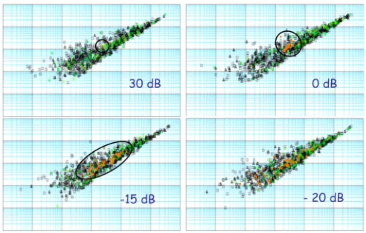
are estimated by n-pass filters and peaks are detected using test defined in (4) with PFA=10-3, 10-4, 10-5, 10-6.

Figure 1 - Error space, etot versus e-3dB, performed with Monte Carlo

simulations of signal sPF(t) at 4 SNRs. Peaks detected at νPF

(whatever the PFA) are figured by orange squares and surrounded by a black ellipsoid except in the -20 dB case, detected peaks at other frequencies with PFA=10-6 by green circles, with PFA=10-5 by

green crosses, with PFA=10-4 by black triangles and with PFA=10-3

by empty black squares.

Figures 1 and 2 show that the proposed error space (e-3dB(p,i),

etot(p,i)) is relevant for discriminating PF and NB signals and

can be used to characterize the associated classes. Black ellipses highlight clusters corresponding to frequency νPF.

These Monte Carlo simulations in the error space are used to define regions, which correspond to different spectral

structures. Indeed these regions are the classes we want to identify.

Figure 2 - Error space, etot versus e-3dB, performed with Monte Carlo

simulations of signal sNB(t) at 4 SNRs. Color codes are the same as

in Figure 1.

We then define a distance, which can be considered as a measure of membership degree of a peak towards a specific class. So as to, at each region delimited by the thresholds shown in Figure 3, we associate an integer distance dkl. Index

k identifies the region and index l a spectral pattern: l=0 for

PF, and l=2 for NB. Class PF is located at low errors under

TPF, defined as a line up to PF cluster at SNR equal to 0 dB.

Figure 3 - Class contours defined from Monte Carlo simulations and parameterized by dkl. Class PF=d00; class NB=d32, class Noise=d31.

Others regions are uncertainty classes.

We characterize it by the minimal distance d00. The more the

errors increase, the more the peak departs from a PF. At the opposite, the noise class is located at high errors above TN,

defined as the line up to PF and NB clusters at SNR equal to -20 dB. We characterize it by a higher distance d31.

Intermediate distances, d11 and d12, measure an uncertainty

between a PF or a noise peak, such as

00 0 11 21 31 d = <d <d <d . (8) 30 dB 0 dB -15 dB - 20 dB 30 dB 0 dB - 20 dB -15 dB TN d11 d d32 d31 d22 d12 d31 TPF 21 d00 TNB Tun

The cluster of NB peaks is located under TN but above TNB,

defined, in the same way, as the line down NB cluster at SNR equal to 0 dB. In this region, we notice a difference compared to PF region because of a possible uncertainty between a NB or a noise peak. The joint PFA defined in section 2.1 is used to discriminate them.. A joint PFA equal to 10-3 or 10-4 will detect a noise peak whereas a joint PFA equal to 10-5 or 10-6 will detect a NB. The studied NB in (7) has a frequency band given by the chosen variance of the corrupting noise ε(t). If this variance decreases, the cluster will go down under TNB and

approaches the PF cluster. Therefore, an increasingly weak distance is associated to the concerned regions such as

. (9)

00 12 22 32

d <d <d <d

with d00 = 0. Between TNB and TPF is a region, which has to

manage an uncertainty between a PF at low SNR and a NB at high SNR. We separate it into two regions, delimited by a line

Tun, which corresponds to the separation between PF and NB

clusters at SNR equal to –15 dB.In the same way as above, the joint PFA is used to separate peaks of different SNR in the same region. Finally, at each couple (k,l) is given a numerical value such as dkl=kd1l, with an initial value d1l. This

classification can be locally extended to multi-component signals embedded in a correlated Gaussian noise. At last, for each γˆp i,

( )

ν , a set of characteristics can be given: the

adjusted central frequency, the time amplitude, the mean noise variance, the local SNR, the emerging SNR which depends upon the estimator, the adjustment errors, a frequency interval

I(CiPp) defined by the –3dB bandwidth as a peak frequency

base, the joint PFA referred to as PFAi and the distance (dkl)i.

This list is referred to as an intermediate card of the peak.

3. SPECTRAL I.D. CARDS AND CLASSIFICATION Intermediate cards are established for each γˆp i,

( )

ν and for

each cycle, i=1,L. A null card, with a distance higher than the value associated to noise, is added when a peak is not detected at one cycle. So as to associate cards corresponding to the same peak, a simple criterion is defined

(10) I(CiPp)∩I(CjPp')≠ ∅, i≠ j

with I(CiPp) being the frequency interval of Peak p in Cycle i. The connected cards form a set called a sequence. Owing to its construction, a sequence describes the same spectral structure, which is also represented by L points in the error space. In each sequence, the intermediate cards are merged according to the following procedure. If the sequence presents more than one uncertainty (non constant index l in dkl over the sequence),

if alarms on PFA (two far PFA are not accepted) or on the noise level were set on, the peak is classified into an Alarm

class, which points out a bad estimate of the noise spectrum. Afterwards, in each sequence, distances are combined as

( )

( )

2 2

1 1

1 L 1 L

peak kl i peak kl i peak

i i

d d and d

L = σ L =

=

∑

=

∑

−d . (11) The final distance dpeak f, is defined as

, , min , peak f peak kl k l d = d d , (12)

and determine the final spectral pattern of the peak. The standard deviation σpeak allows the computation of a stability

index Stpeak, which indicates the stability of the results on the

sequence with a known maximum standard deviation σmax,

(

max

)

100 1

peak peak

St = −σ σ . (13)

A final PFA, PFApeak, is calculated as

(

)

1 1 = =

∏

L L peak i i PFA PFA . (14)

The final card is called the spectral I.D. and gathers these new characteristics. The final distance dpeak is used to classify all

the peaks in one of the following classes: PF, NB, Alarm and Noise. Finally, it is important to notice that the detection probability of a peak is high if the classification yields a high stability index Stpeak and a low final PFA PFApeak

simultaneously.

In order to underline this property, a simulation is carried out on a signal s(t) computed as the sum of one NB as defined in (7) and two PF as defined in (6),

( )

= NB

( )

+ PF1

( )

+ PF2

( )

s t s t s t s t . (15) The parameters of the NB are unchanged, νNB = 110 Hz and

ANB=10. The first PF is located at νPF1 = 112 Hz, close to the

NB, but with an amplitude ten-fold weaker, APF1=10. The

second one, at νPF2 = 180 Hz, is separated from the others but

at a lower amplitude, APF2=0.4. The global signal to noise ratio

is 10 dB.

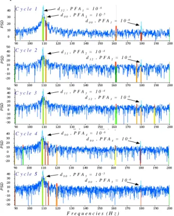
Figure 4 presents L=5 complementary spectral analyses (an hybrid periodogram-correlogram with Blackman window, a Welch-Wosa first with Blackman window then with Hanning window, a Blackman-Tuckey first with Blackman window then with Hanning window [4]). For sake of simplicity, only a zoom between 90 Hz and 200 Hz is shown. The colored peaks correspond to the peaks detected by test (4). As can be seen, the different estimated PSDs do not lead to the same detected peak set, reinforcing the idea of using jointly all these different analyses. The only peak, which is detected in the same way

through all cycles, is the NB one at νNB = 110 Hz with a joint PFA equal to 10-6. PS D F r e q u e n c i e s ( H z ) C y c l e 1 C y c l e 2 C y c l e 3 C y c l e 4 C y c l e 5 d3 2, P F A1= 1 0- 6 d0 0, P F A1= 1 0- 5 d0 0, P F A1= 1 0- 6 d1 1 , P F A2= 1 0- 4 d1 2 , P F A2= 1 0- 6 d1 1, P F A3= 1 0- 4 d1 2 , P F A3= 1 0- 6 d0 0, P F A4= 1 0- 6 d0 0 , P F A4= 1 0- 6 d0 0 , P F A5= 1 0- 5 d0 0 , P F A5= 1 0 - 6 PS D P SD PSD PS D

Figure 4 – Zoom spectra of signal s(t) for L cycles with L=5

To derive spectral I.D. cards based on these 5 cycles, it is necessary to take into account the stability index (13) and the final PFA (14), presented in Figure 5. The NB structure is detected with a stability index of 100% and a low mean PFA of 10-6. Indeed, only high stability indexes have to be considered since they correspond to a consensus in the different spectral analyses, together with low final PFAs. With the NB signal, this occurs only at 112 Hz and 180 Hz, frequencies of sPF1 and sPF2.. Moreover, in this signal

realization, the final PFAs are rather high, except for the 3 structures of interest and for two other high frequency peaks, surrounded by a red ellipsoid. However, their related stability indexes are null, showing that the different analyses lead to unstable results.

4. CONCLUSION

The strategy of spectral analysis presented in this paper leads to an automatic process for detecting, characterizing and classifying sinusoidal waves and narrow band signals of an unknown stationary process. This kind of tool is of interest when needing a fast and outstanding analysis of signals. The idea of fusion of different spectral analysis methods is original in signal analysis field. Operating spectral estimator properties allows a rigorous and accurate identification of spectral peaks,

which breaks free from a visual interpretation. It is important to note that the proposed classification was derived from a particular stationary NB process. Works are in progress to extend these results to other NB models and to validate the last step of card fusion.

S ta b ilit y In d e x Fi n a l PF A 0 1 0 0 % 1 0-6 1 0-5 1 0-4 1 0-3 1 0-2 1 0-1 D e te c te d p e a k in d e x (n o n lin e a r fr e q u e n c y s c a le ) 1 1 0 H z 1 1 2 H z1 8 0 H z

Figure 5 – Stability Index and final PFA of signal s(t) for all the detected peaks.

5. REFERENCES

[1] J. Schoukens, Y. Rolain, G. Simon, R. Pintelon, Fully

automated spectral analysis of periodic signals, IEEE Tr. Ins. Meas., Vol 52, n°4, August 2003, pp.1021-1024.

[2] L-M. Zhu, H-X. Li, H. Ding, Estimation of multi-frequency

signal parameters by frequency domain non-linear least squares, Mech. Syst. and Sig. Proc., Elsevier, Vol. 19, 2005, pp. 955-973.

[3] D. Rabijns, G. Vandersteen, W. Van Moer, An automatic

detection scheme for periodic signals based on spectrum analyzer measurements, IEEE Trans Instr. Measur., vol 53, n°3, June 2004.

[4] M. Durnerin, Une stratégie pour l’interprétation en analyse

spectrale, détection et caractérisation des composantes d’un spectre, INPG PhD thesis, September 1999, www.lis.inpg.fr.

[5] N. Martin, C. Mailhes, K. Sahli, G. Lejeune, Vers une Carte

d'Identité Spectrale, 20ème colloque GRETSI sur le Traitement du Signal et des Images, Louvain-la-Neuve, Belgique, Sept. 6-9, 2005.

[6] P.E. Johnson and D.G. Long, The Probability Density of

Spectral Estimates Based on Modified Periodogram Averages. IEEE Trans. on SP, Vol. 47, n°. 5, May 1999, pp.1255-1261.

[7] W.A. Struzinski, E.D. Lowe, A performance comparison of 4

noise background normalization schemes proposed for signal detection systems. JASA., n°. 78, Sept. 1985, pp. 936-941.

[8] L.O Hoeft, J.L. Knighten, J.T. DiBene II; M.W. Fogg, Spectral

analysis of common mode currents on fibre channel cable shields due to skew imbalance of differential signals operating at 1.0625 Gb/s, IEEE Int. Symp. on EC, Vol. 2, 24-28, Aug. 1998.

[9] M. Drinnan, J. Allen, P. Langley, A.Murray, Detection of sleep

apnoea from frequency analysis of heart rate variability, Computers in Cardiology 2000, 24-27 Sept. 2000, pp. 259-262.

[10] N. Martin, P. Jaussaud, F. Combet, Close shocks detection using time-frequency Prony Modelling. MSSP, Mechanical Systems and Signal Processing, Vol. 18, n°2:, March 2004. pp. 235-261