HAL Id: hal-01100420
https://hal.inria.fr/hal-01100420
Submitted on 6 Jan 2015
HAL is a multi-disciplinary open access
archive for the deposit and dissemination of
sci-entific research documents, whether they are
pub-lished or not. The documents may come from
L’archive ouverte pluridisciplinaire HAL, est
destinée au dépôt et à la diffusion de documents
scientifiques de niveau recherche, publiés ou non,
émanant des établissements d’enseignement et de
Convergecast in IEEE 802.15.4e Networks (Extended
Version)
Ridha Soua, Pascale Minet, Erwan Livolant
To cite this version:
Ridha Soua, Pascale Minet, Erwan Livolant. Wave: a Distributed Scheduling Algorithm for
Con-vergecast in IEEE 802.15.4e Networks (Extended Version). [Research Report] RR-8661, Inria. 2015,
pp.32. �hal-01100420�
ISRN
INRIA/RR--8661--FR+ENG
RESEARCH
REPORT
N° 8661
Scheduling Algorithm for
Convergecast in
IEEE 802.15.4e Networks
(Extended Version)
RESEARCH CENTRE PARIS – ROCQUENCOURT
(Extended Version)
Ridha Soua, Pascale Minet, Erwan Livolant
Project-Teams Hipercom2
Research Report n° 8661 — January 2015 — 32 pages
Abstract: Wireless sensor networks (WSNs) play a major role in industrial environments for data gathering (convergecast). Among the industrial requirements, we can name a few like 1) determinism and bounded convergecast latencies, 2) throughput and 3) robustness against inter-ferences. The classical IEEE 802.15.4 that has been designed for low power lossy networks (LLNs) partially meets these requirements. That is why the IEEE 802.15.4e MAC amendment has been proposed recently. This amendment combines a slotted medium access with a channel hopping (i.e. Time Slotted Channel Hopping TSCH). The MAC layer orchestrates the medium accesses of nodes according to a given schedule. Nevertheless, this amendment does not specify how this schedule is computed. The purpose of this paper is to propose a distributed joint time slot and channel assignment, called W ave for data gathering in LLNs. This schedule targets minimized data convergecast delays by reducing the number of slots assigned to nodes. Moreover, W ave ensures the absence of conflicting transmissions in the schedule provided. In such a schedule, a node is awake only during its slots and the slots of its children in the convergecast routing graph. Thus, energy efficiency is ensured. In this paper, we describe in details the functioning of W ave, highlighting its features (e.g. support of heterogeneous traffic, support of a sink equipped with multiple interfaces) and properties in terms of worst case delays and buffer size. We discuss its features with regard to a centralized scheduling algorithm like T MCP and a distributed one like DeT AS. Simulation results show the good performance of W ave compared to T MCP . Since in an industrial environment, several routing graphs can coexist, we study how W ave supports this coexistence.
Key-words: Wireless sensor network, IEEE 802.15.4e, conflict-free schedule, convergecast, sched-uled access, multichannel, time slot, channel allocation, multiple interfaces, data gathering
(Version Etendue)
Résumé : Les réseaux de capteurs sans fil jouent un rôle majeur pour la collecte de données dans les environnements industriels. Parmi les exigences industrielles visées, nous pouvons citer 1) le déterminisme et les latences de collecte bornées, 2) le débit et 3) la robustesse vis-à-vis des interférences. La norme IEEE 802.15.4 classique, qui a été conçue pour les réseaux avec pertes et contraintes énergétiques (ou Low power Lossy Networks, LLNs), ne répond que partiellement à ces exigences. C’est pourquoi l’amendement IEEE 802.15.4e a été proposé récemment. Cet amendement propose un mode d’utilisation TSCH (Time Slotted Channel Hopping) combinant l’accès au médium par slots temporels et le saut de fréquence. La couche MAC orchestre les accès au médium des nœuds du réseau selon un ordonnancement donné. Néanmoins, l’amendement ne spécifie pas comment cet ordonnancement est calculé. Le propos de ce papier est d’offrir un algorithme distribué d’assignation conjointe de fréquences et de slots temporels pour la collecte dans les LLNs, dénommé W ave. Cet ordonnancement vise à minimiser le temps de collecte en réduisant le nombre de slots temporels assignés à l’ensemble des nœuds du réseau. De plus, W aveassure l’absence de transmissions conflictelles dans l’ordonnancement fourni. Dans un tel ordonnancement, un nœud est réveillé uniquement pendant ses slots de transmissions et ceux de ses enfants dans le graphe de routage de la collecte. Ainsi, l’efficacité énergétique est assurée. Dans ce papier, nous décrivons en détails le fonctionnement de W ave, mettant en exergue ses caractéristiques (support du trafic hétérogène, support d’un puits de données avec de multiples interfaces de communication) et ses propriétés en terme de délais et de la taille des buffers. Nous discutons ses caractéristiques en regard d’un algorithme d’ordonnancement centralisé tel que T M CP et d’un autre distribué tel que DeT AS. Les résultats de simulations démontrent une meilleure performance de W ave par rapport à T MCP . Enfin, puisque dans un environnement industriel plusieurs graphes de routage peuvent cohabiter, nous étudions comment W ave assure cette coexistence.
Mots-clés : Réseau de capteurs sans fil, IEEE 802.15.4e, ordonnancement sans conflit, col-lecte de données, accès ordonnancé, multicanal, slot temporel, allocation de canaux, interfaces multiples
Contents
1 Introduction 4
1.1 Low power Lossy Networks (LLNs) . . . 4
1.2 Raw Data Convergecast problem . . . 4
1.3 IEEE 802.15.4e TSCH . . . 5
1.4 Industrial use cases . . . 5
2 State of the art 6 2.1 Theoretical work . . . 6
2.2 Scheduling algorithms . . . 7
2.2.1 Centralized algorithms . . . 7
2.2.2 Distributed algorithms . . . 8
3 Network model and preliminaries 9 3.1 Network model . . . 9
3.2 Routing graph . . . 9
3.3 Acknowledgment policy . . . 9
3.4 Conflict model . . . 9
3.5 Traffic model . . . 11
4 The Wave scheduling algorithm 11 4.1 Principles and algorithm of W ave . . . 11
4.1.1 Illustrative example . . . 12
4.1.2 Computation of the first wave . . . 13
4.1.3 Local computation of the slots assigned in the next waves . . . 14
4.1.4 Algorithm of W ave . . . 14
4.2 Properties of W ave . . . 14
4.3 Analytical results: delays, buffer size and messages . . . 16
4.3.1 Computation of the worst case data gathering delays . . . 16
4.3.2 Computation of the buffer size . . . 16
4.3.3 Messages exchanged by Wave and by a centralized algorithm . . . 17
4.3.4 Computational complexity of Wave . . . 18
5 Evaluation of the flexibility of W ave 19 5.1 Simulation parameters . . . 19
5.2 Homogeneous traffic . . . 19
5.3 Support of additional links . . . 19
5.4 Support of heterogeneous traffic demands . . . 20
5.5 Support of a sink with multiple radio interfaces . . . 21
5.6 Support of different acknowledgment policies . . . 22
5.7 Support of service differentiation . . . 23
6 Impact of dynamic changes on the conflict-free schedule 24 6.1 Impact of retransmissions or changes in application needs . . . 24
7 Support of multiple routing graphs 26
7.1 Independent routing graphs . . . 27
7.2 Dependent routing graphs . . . 27
7.2.1 General principles . . . 27
7.2.2 Illustrative example . . . 29
1
Introduction
1.1
Low power Lossy Networks (LLNs)
The spectacular interest for the Internet of Things has boosted the deployment of Low power Lossy Networks (LLNs). LLNs are composed of many tiny low-cost low-power on-chip devices. These latter have limited memory and processing resources. They are interconnected by a variety of technologies, such as IEEE 802.15.4, WiFi or Bluetooth. Short communication ranges and limited bandwidth of nodes lead to multi-hop communications and low data rates. LLNs use medium access (MAC) protocols with restricted frame size. Therefore, scheduling techniques should be specifically adapted for such MAC layers.
LLNs have gained widespread usage in many applications, including target tracking, envi-ronmental monitoring, health monitoring, smart homes, industrial monitoring. This can be explained by the easy deployment of wireless sensor networks. These networks are a typical example of LLNs.
1.2
Raw Data Convergecast problem
Data collection represents a significant fraction of network traffic in many industrial applications. The individual devices sense their surrounding environment and send their data, directly or via multiple hops, to a central device, namely the sink, for processing. Every node plays the role of data source and/or router node through a routing graph to deliver packets to the sink without agregation by intermediate routers. This data collection is called raw data convergecast. Raw data convergecast is particularly well suited for applications with low correlation level between the data gathered and/or for LLNs with a reduced payload at the MAC level. In this context, nodes that are near the sink should forward more packets than sensors far away. Hence, the scheduling of transmissions should be traffic-aware. Nevertheless, data convergecast raises two challenges: 1) time efficiency and 2) energy efficiency.
The former challenge is crucial in industrial environment that generally requires small delays and time consistency of data gathered. This time consistency is usually achieved by a small gathering period. In fact, minimized end-to-end delays ensure freshness of collected data. As argued in [1], using multichannel techniques ensures parallel transmissions and higher capacity. Therefore, the data gathering delays can be reduced drastically. Moreover, limiting factors for a fast data collection are interferences. To mitigate this problem, authors in [1] argued that resorting to multichannel communications is more efficient than varying transmission power. Meanwhile, the new standard IEEE 802.15.4e [2] uses channel hopping to minimize interferences. In addition, when two or more nodes send their data to a common parent at the same time, the messages collide at the common parent. Hence, the parent will not receive data from any senders. This situation is more challenging in convergecast applications because a large number of nodes, that may transmit simultaneously, is involved. Thus, collisions represent a major challenge for bounded latencies and deterministic packet delivery times.
Energy efficiency, the latter issue, is challenging in LLNs because nodes are battery operated. The heavy traffic drastically increases the probability of collisions and retransmissions. Therefore, contention-based medium access protocols are inefficient for periodic data collection. In contrast, contention-free protocols schedule interfering nodes in different slots. Each node transmits data in its allocated slots. Contention-free protocols are the preferred access scheme for applications that require energy efficiency and bounded end-to-end delays. On the one hand, these protocols remove idle listening and overhearing, which are the main sources of energy drain in contention-based protocols. Thus, the provided schedule is appropriate for low power devices since nodes turn off their radio in non scheduled time slots. This contributes to energy efficiency and network
lifetime prolongation. On the second hand, contention-free protocols have the ability to deliver packets with deterministic delay bounds by eliminating collisions and retransmissions. Indeed, WirelessHART [3], a standard for control applications, uses a TDMA data link layer to control medium access.
1.3
IEEE 802.15.4e TSCH
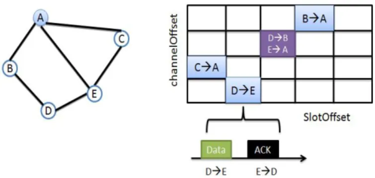
The IEEE 802.15.4 standard does not meet all requirements of industrial applications supported by LLNs, more particularly in terms of robustness against interferences and throughput. For instance, the use of a single channel does not solve the problem of interferences in a deterministic way and may not meet the throughput required by such applications. The MAC amendment, IEEE 802.15.4e Time Slotted Channel Hopping (TSCH) [2] was proposed in 2011 to better meet industrial markets requirements. This amendment extends the classical IEEE 802.15.4e standard to make it suitable for low-power multi-hop networks: the TSCH mode ensures robustness and high reliability against interferences by channel hopping. A given node sends subsequent packets on different channels. Hence, interferences and multipath fading are mitigated. In the TSCH mode, nodes are synchronized and follow a schedule using a slotframe structure. A slotframe is a group of time slots which repeats over time, as depicted in Figure 1. The number of time slots per slotframe is tunable.
Figure 1: IEEE 802.15.4e TSCH slotframe
Each node accesses the medium following a communication schedule. This latter is a matrix of cells, each of them is indexed by a slot offset and a channel offset. Each cell can be assigned to a link defined by its transmitting and receiving nodes. A scheduled cell can be shared between multiple links or dedicated to only one link. As illustrated by Figure 2, the blue cells are dedicated cells while the purple cell (darker cell) depicts a shared cell. A single slot is long enough for the transmitter to send a maximum length packet and for the receiver to send back an acknowledgment.
However, the IEEE 802.15.4e TSCH standard does not propose a mechanism to build the schedule but defines only how the MAC layer executes it. In this paper, we cover this gap by proposing W ave, a distributed scheduling algorithm that jointly optimizes the channel and time slot assignment in LLNs. This algorithm is tailored for convergecast applications and ensures minimized data gathering delays.
1.4
Industrial use cases
The technology of wireless sensor networks is now able to provide multichannel and determinism support. Determinism will support 1) bounded delays for data gathering and 2) energy efficiency because the medium accesses are done without collision and since each node knows when it will transmit and receive data, it sleeps the remaining time to save energy. 3) Throughput and 4) robustness against interferences are supported mainly by multichannel and partly by
Figure 2: IEEE 802.15.4e TSCH schedule
determinism. These four application requirements are declined in the following six use cases in industrial applications, as illustrated by Table 1 where M stands for Mandatory, O for Optional (it depends on the application) and N for No.
Table 1: Industrial use cases
Use cases Robustness Throughput Low cost Bounded delays Energy efficiency
Temporary worksite monitoring M O O M M
Detection of fire, pollutant or leak M N M M O
Industrial process optimization O M M O O
Predictive maintenance M O M O O
Intruder detection M O O M N
Aerospace application M O N M M
The remaining of this paper is organized as follows. In Section 2, we present relevant work that focuses on theoretical bounds for convergecast, centralized and distributed scheduling algorithms. In Section 3, we give the network, traffic and conflict models. Section 4 describes the behavior of W ave. A performance evaluation is conducted in Section 5 to compare W ave with T MCP . In Section 6, we study the impact of changes in traffic or in the routing graph. The support of multiple routing graphs is discussed in Section 7. Finally, Section 8 concludes the paper and gives some perspectives.
2
State of the art
2.1
Theoretical work
The following fundamental question: “what is the minimum number of slots we need to collect raw data from a LLN organized in a tree?” has been investigated in many studies. Nevertheless, they have specifically targeted the simple case where sensors generate only one packet. In [4], authors address jointly the link scheduling and channel assignment for convergecast in networks operating according to the WirelessHART standard. Authors have proved that for linear networks with N single buffer devices, the minimum schedule length obtained is (2N − 1) time slots with dN/2e channels.
Incel et al. [1] have proved that if all interfering links except those belonging to the routing tree are removed (with the required number of channels), the schedule length for raw-data con-vergecast is lower bounded by max(2nk− 1, N )where nk is the maximum number of nodes in
extend this work by considering the case where the sink is equipped with multiple radio inter-faces and nodes generate heterogeneous traffic. Indeed, in any linear LLN with heterogeneous demands of nodes, where each node has nchannel > 1, the minimum number of slots for a raw data convergecast is Gen(ch1)+2 Pu6=sink,u6=ch1Gen(u), whatever the number of interfaces that
the sink has, where Gen(u) is the number of slots needed by node u to transmit its own data to its parent and ch1 is the most transmitting child of the sink.
In multilines or tree networks with heterogeneous demands of nodes, a lower bound on the number of slots for a raw data convergecast is Max(Sn,St), where:
• Sn = d P
u6=sinkGen(u)
g e, where g = min(nchild, nchannel, ninterf).
• St= Gen(ch1) + 2Pv∈ Subtree(ch1),v6=ch1(Gen(v)) + δ, where ch1 is the most transmitting
child of the sink and δ = 1 if the (g + 1)th child of the sink requires the same number of
transmissions as the first one, and δ = 0 otherwise. We define two types of configurations:
• Tt configurations where the optimal number of slots is imposed by the most demanding
subtree rooted at a sink child, i. Its demand is equal to Gen(i)+2 Pv6=i,v∈subtree(i)Gen(v).
The Ttconfigurations are dominated by the subtree requiring the highest number of
trans-missions.
• Tn configurations where the optimal number of slots depends only on the total number of
demands and g. It is equal to dPu6=sinkGen(u)
g e. The Tnconfigurations are traffic-balanced.
Notice that a Tn configuration corresponds to a Capacitated Minimal Spanning Tree [6],
where each branch has a total demand for slots less than or equal to dPu6=sinkGen(u)
g e.
2.2
Scheduling algorithms
To schedule nodes in multichannel context, two approaches can be distinguished. The first ap-proach starts with a channel allocation. Channels are usually allocated to receivers or links. Then, the time slot assignment is triggered. Interferences, that are not removed by channel allo-cation, are avoided by assigning different time slots to concurrent senders. The second approach jointly allocates channels and slots. Hereafter, we will detail the most relevant centralized and distributed scheduling algorithms for data gathering in multichannel context.
2.2.1 Centralized algorithms
TMCP [7] is designed to support data collection traffic. It begins by partitioning the network into multiple subtrees and then assigns different channels to nodes belonging to different subtrees. Hence, it minimizes interferences between subtrees. After the channel assignment, time slots are assigned to nodes. However, TMCP does not eliminate contention inside the branches of a subtree since nodes that belong to the same branch communicate on the same channel.
Incel et al. [1] propose a convergecast scheduling algorithm, called JFTSS, that achieves optimal bound on any network topology where the routing tree has an equal number of nodes on each branch and each node generates the same amount of traffic (i.e. all nodes have the same sampling rate).
Authors of [8] propose TASA, a centralized traffic-aware scheduling algorithm for networks based on IEEE 802.15.4e. TASA proceeds in two steps: 1) a matching step where links eligible to be scheduled in the same time slot are selected 2) a coloring step where each link selected for
transmission is assigned a channel offset. The channel offset is translated into a frequency using a translation function. However, TASA does not take into account queue congestion in sensor nodes, leading to large buffer size at these nodes.
In [9], authors design MODESA, a Multichannel Optimized DElay time Slot Assignment. This latter is a centralized collision-free algorithm that takes advantages from multiple channels to allow parallel transmissions and improve communication reliability. Authors prove the optimality of MODESA in many multichannel topologies of wireless sensor networks. In addition, MODESA reduces buffer congestion by scheduling first the nodes that have more packets in their buffers.
Although in distributed scheduling strategies it is difficult for each node to find an optimal schedule because global information is unavailable, these solutions are considered more attractive in large scale networks and more reliable than a centralized one. We will detail most relevant distributed solutions in the next section.
2.2.2 Distributed algorithms
In [10], Incel et al. derive a TDMA schedule that minimizes the number of slots required for convergecast. They extend the distributed algorithm proposed by Ghandam et al. [11] to the context of multichannel wireless sensor networks. Their approach includes two steps: 1) A receiver based channel assignment: it removes all the interference links in an arbitrary network. 2) A distributed slot assignment: where each node is assigned an initial state (i.e. transmit Tx,
receive Rxor idle) based on its hop-count to the sink and the state of its branch. If the branch
is active (i.e. the sink child located in the top of the branch transmits), a node with hop-count his assigned state Tx if h mod 2 = 1 and state Rx otherwise. If the branch is not active, it is
assigned state Txif h mod 2 = 0 and Rxotherwise. In the next slot, nodes switch to the opposite
state.
The algorithm does not specify how slots are assigned to brothers. Besides, the authors assume that after channel allocation, the only remaining conflicts are inside the convergecast tree. They also show that this algorithm is optimal when all interferences are removed using the necessary number of channels and a suitable balanced routing tree is built.
Accettura et al. [12] propose DeTAS, a distributed traffic aware scheduling solution for IEEE 802.15.4e TSCH networks. This solution is the distributed mode of TASA proposed in [8]. In DeTAS, all nodes follow a common schedule, called macro-schedule, that is the combination of micro-schedules of each routing graph. Each micro-schedule is computed in distributed manner. DeTAS avoids buffer overflow by alternating the sequence of transmit/receive slots for each node. However, if other links exist in addition to the convergecast links, collisions may occur.
Authors of [17] propose W ave, an algorithm that schedules nodes in successive waves. In each wave, each node having a packet to transmit is assigned a time slot and a channel. The first wave constitutes the (slot, channel) pattern. Each next wave is an optimized subset of the first wave: only the slots that will contain transmissions are repeated and they always occur in the same order as in the first wave. To know its next scheduled slots, a node applies a simple rule. As a result, the joint channel and time slot assignment produced by W ave contains for each time slot and for each available channel, a list of sender nodes, such that their transmissions to their parent do not conflict.
Morel et al. [13] map multiprotocol label switching to constrained LLN to provide distributed scheduling for IEEE 802.15.4e networks. Indeed, nodes request bandwidth in terms of time slots. The RSVP-TE over GMPLS protocol ensures that reserved network resources match the requirements of nodes. Their solution, CFDS, has two components: (1) a time slot mechanism that prevents a node to be involved either in two simultaneous transmission and reception, or two simultaneous receptions; this mechanism is the request and the grant procedure; (2) a channel
offset selection mechanism that mitigates internal and external interferences.
3
Network model and preliminaries
3.1
Network model
We focus on raw data gathering in LLNs based on the IEEE 802.15.4e standard. The data gathered are transmitted by nodes different from the sink in the slotframe according to the schedule provided by the W ave scheduling algorithm that we will present in the next section. Furthermore, we assume that any node u 6= sink receiving a packet in slot t is able to forward it in the slot t + 1 if required by the schedule. A slot contains one packet. If the immediate acknowledgment policy is used (see Subsection 3.3), a slot also contains the acknowledgment of the data packet sent. In all cases, the slotframe is dimensionned to enable the transfer of all packets generated during the slotframe. The problem is to minimize the number of slots composing the slotframe.
3.2
Routing graph
Network connectivity is assumed. For any data gathering considered, the associated routing graph is given. It can be a DODAG provided by RPL [14] or a routing tree provided by a gradient method such as EOLSR [15] or [16]. The root of this routing graph is the sink in charge of gathering data produced by sensor nodes. Each node u 6= sink has a unique preferred parent that is abusively called parent in this paper.
3.3
Acknowledgment policy
Two acknowledgment policies are studied:
• either there is no acknowledgment: since we consider a lossy network, the probability of packet loss is not neglectable. This policy can be adopted only if the packet loss rate is acceptable for the application.
• or there is an immediate acknowledgment: each data packet is acknowledged in the same time slot and on the same frequency it has been sent. If the immediate acknowledgment policy is used, the routing tree consists only of symmetric links.
3.4
Conflict model
Two nodes u and v are said to conflict if and only if they cannot transmit in the same time slot and on the same channel frequency without preventing: 1) either a destination node to correctly receive its data packet 2) or a sending node to receive the acknowledgment of its data packet. Notice that this definition depends on the acknowledgment policy used. If there is no acknowledgment, only the item 1) is relevant.
In the literature, there are two types of conflict models: those based on the topology graph, also called protocol-based and those based on a physical model (e.g. SINR measures). With both types of models, a conflict graph is built. This graph is more accurate if it takes into account the feedback provided by physical measures (e.g. SINR, LQI, RSSI). It is important to notice that W ave takes the conflict relation as an input, provided that this relation is symmetric. If a physical model is adopted, W ave must know for each conflicting node a path to reach it. In the following of this paper, we adopt a protocol-based model of conflicts.
In a protocol-based model of conflicts, the conflict relation is built from the one-hop neighbor relation. Two nodes are said one-hop neighbors if and only if they hear each other. We can now recursively define the h-hop neighbor relation, with h > 1. Two nodes u and v are h-hop neighbors, with h > 1, if and only if there exists a one-hop neighbor of u that is (h-1)-hop neighbor of v.
In the absence of acknowledgment, the only possible conflicts are caused by the simultaneous transmissions of two data packets as depicted in Figure 3. In this figure, links used for data gathering are the tree links and are depicted in black plain line, whereas blue dotted lines represent links between one-hop neighbors that are not used in the routing tree. It is worth noting that such links may cause collisions. For instance, when node 3 is transmitting data to its parent, node 2 that is a one-hop neighbor of node 1 = parent(3) cannot transmit: it would prevent node 1 to receive correctly, even if link (2,1) does not belong to the tree. All circled nodes are conflicting nodes.
Figure 3: Conflicting nodes of node 3 without acknowledgment.
Property 1 In this graph-based model and in the absence of acknowledgment, the nodes con-flicting with any node u are:
- the node u itself, - its parent P arent(u), - its children,
- the nodes that are 1-hop away from P arent(u), - the nodes whose parent is 1-hop away from u.
When the immediate acknowledgment policy is chosen, there are additional conflicts. They are caused by the simultaneous transmissions of a data packet and an acknowledgment, as de-picted in Figure 4. In this figure, a black arrow represents the transmission of a data packet, whereas a red arrow denotes the transmission of an acknowledgment packet. A dotted line represents a link without intended transmission.
Property 2 In this graph-based conflict model, the nodes conflicting with any node u are for the immediate acknowledgment policy:
- the node u itself, - its parent P arent(u),
- the nodes that are 1-hop away from u or P arent(u), - the nodes whose parent is 1-hop away from u or P arent(u).
Figure 4: Conflicting nodes with the immediate acknowledgment.
In the absence of acknowledgment, the set of conflicting nodes, defined by Property 1, is included in the two-hop neighbors set. With the immediate acknowledgment, the set of conflicting nodes, defined by Property 2, is included in the three-hop neighbors set.
Property 3 In the graph-based conflict model, the nodes conflicting with any node u with the immediate acknowledgment are those without acknowledgment, in addition to:
- the nodes that are 1-hop away from u but are not its children, - the nodes whose parent is 1-hop away from P arent(u).
3.5
Traffic model
Any node u 6= sink generates Gen(u) ≥ 1 packets in each slotframe. These packets contain the own data of u. They are assumed to be present when the data gathering is started and are renewed in each slotframe. Two nodes u and v may generate different traffic loads (i.e. Gen(u) 6= Gen(v)). Furthermore, T rans(u) denotes the total number of packets transmitted by uin a slotframe. This corresponds to the own packets of u and the packets transmitted by its children. Consequently, we have T rans(u) = Gen(u) + Pv∈Child(u)T rans(v).
4
The Wave scheduling algorithm
In this section, we detail W ave a simple distributed conflict-free scheduling algorithm in networks based on IEEE 802.15.4e. W ave supports a sink with multiple radio interfaces, heterogeneous traffic and additional links to the convergecast tree. It can be extended as shown in Section 7 to support several routing graphs.
A schedule is said valid if and only if two conflicting nodes do not transmit in the same time slot and on the same channel frequency.
The goal of W ave is to compute a valid schedule that minimizes the number of slots allocated while ensuring that:
• each node has the number of slots needed to forward any packet received from its children and to send its own packets;
• and each packet transmitted in a slotframe reaches the sink in the same slotframe.
4.1
Principles and algorithm of W ave
In W ave, any node u 6= sink needs to know its parent and its children in the routing graph consid-ered, the acknowledgment policy, the nodes conflicting with u whose set is denoted Conflict(u), the traffic demand of u and all nodes in Conflict(u).
W aveproceeds in successive waves: the ithwave schedules the ith transmission of any node
having at least i packets to transmit. In the first wave, each node is assigned a time slot and a channel frequency to transmit one packet. This first wave is computed in order to minimize the total number of slots needed. Next, this wave is reproduced but in an optimized way: only the slots that are needed by at least one node are reproduced in the next wave. The total number of waves in the schedule is equal to W = maxu6=sinkT rans(u).
4.1.1 Illustrative example
Figure 5a depicts a routing graph including nine nodes, where node 1, the sink, is equipped with a single interface. The number in the bullet denotes the number of packets transmitted by the node in a data gathering cycle. The schedule provided by W ave is depicted in Figure 5b. It consists of four waves, since maxu6=sinkT rans(u) = 4.
a Routing graph
b Associated schedule
Figure 5: Wave on an example.
The first wave comprising 3 slots allows each node to transmit one packet without collision. It is built considering nodes in the decreasing order of their number of transmissions: in this example, the order is 2, 5, 3, 4, 8, 6, 7, 9. A node is assigned the first time slot and channel where itself and its parent have an available interface and it does not conflict with the nodes already scheduled in this slot and on this channel. The second wave comprises 3 slots too, but nodes 6, 7 and 9 that had only one packet to transmit are no longer scheduled. In other words, the
second wave reproduces the first wave eliminating nodes that have strictly less than 2 packets to transmit. In the third wave, the third slot would be empty (node 4 has already transmitted all its packets), this slot is eliminated. Hence the size of the third wave is equal to 2 slots. And so on, until the fourth wave that contains only one slot used by node 2. In Figure 5b, we represent under each wave, the part of the routing graph that is scheduled in this wave. It appears that nodes having only one remaining packet to transmit in the current wave are eliminated in the next wave (e.g. node 5 present in the third wave is eliminated in the fourth wave).
4.1.2 Computation of the first wave
The sink sends a Start message down the routing graph to trigger the computation of the schedule for this routing graph. More specifically, in the first wave, each node computes its time slot and channel frequency according to the following rules R1 and R2.
Rule R1 : Any node u 6= sink having received the Start message and having the highest priority (i.e. the highest number of transmissions) among its conflicting nodes not yet scheduled, assigns itself a time slot and a channel frequency. The slot selected by u is the first available time slot where:
- both u and its parent have an available interface,
- there is a channel frequency where u does not conflict with the nodes already scheduled in this time slot and on this channel frequency.
Rule R2 : As soon as node u is assigned a time slot and a channel frequency, it notifies this assignment to its conflicting nodes by the Assign message.
The Assign message is forwarded according to the following property.
Property 4 Any node u receiving the Assign message originated from node v forwards it if and only if:
• in the absence of acknowledgment, u is a parent and u is one-hop away from v;
• in the presence of the immediate acknowledgment, u is a parent and u is one-hop away from v or P arent(v).
Proof: When v is scheduled, it sends its Assign message. This message in the absence of loss is received by any one-hop neighbor of v, in particularly by its parent and its children. Any node that receives it and is a parent forwards it. Hence, in the absence of acknowledgment and message loss, all nodes that conflict with v that are defined in Property 1 know the slot and channel assignment of v. Hence, the first part of the property.
With the immediate acknowledgment policy, there are other nodes that forward the Assign message originated from v. These other nodes are parent nodes one-hop away from P arent(v), which have received the message from P arent(v). Hence, all nodes defined in Property 2 know the slot and channel assignment of v. Hence, the second part of the property.
To compute the next waves, it is needed to know the number of slots of the first wave, as well as the repetition factor of each slot. To this end, the following rule R3 is applied.
Rule R3 : Any node that has no child and knows the slots and channel frequency of its conflicting nodes sends a Notify message to its parent, containing for each time slot t that it knows its repetition factor Maxtrans(t). Upon receipt of the Notify message from each of its children, a node u 6= sink sends its Notify message to its parent. The sink sends back down the routing graph a Repeat message including T the number of slots composing the first wave and for each slot 1 ≤ t ≤ T its repetition factor Maxtrans(t).
4.1.3 Local computation of the slots assigned in the next waves
Upon receipt of the Repeat message, any node is able to compute locally its slot and the slot assigned to each conflicting node in any wave w > 1, by applying rule R4.
Rule R4 :Any node u 6= sink being assigned the slot t in the first wave is also assigned the slot s(t, w)in any wave w with 1 < w ≤ T rans(u), with s(t, w) = Pw−1w0=1
PT
t0=1δt0,w0+Pt
t0=1δt0,w, where δt0,w0 = 1 if and only if Maxtrans(t0) ≥ w0 and 0 otherwise, where Maxtrans(t0)is the maximum number of transmissions of any node transmitting in the time slot t0.
4.1.4 Algorithm of W ave
The algorithm for the computation of the first wave is given in Algorithm 1. After some initial-izations, the local node u starts by sorting its conflicting nodes according to the decreasing order of their number of transmissions (see line 6). Then node u enters a loop (lines 8 to 40) until all conflicting nodes are scheduled. This loop consists of two parts:
• the processing of the Assign message received that notifies the time slot and channel assigned to node v (line 11). If v is a conflicting node of u, u updates different variables such as the list of conflicting nodes to schedule, the number of available interfaces of its parent, etc. In any case, u forwards the Assign message according to Property 4 in order to notify all nodes conflicting with v.
• the scheduling of node u as soon as it has the highest priority among its conflicting nodes not yet scheduled (lines 13 to 39). Node u is assigned the smallest time slot where u and its parent have an available interface (lines 19 to 21) and then the smallest channel on which udoes not conflict with the nodes already scheduled (lines 22 to 37).
4.2
Properties of W ave
With the assumptions given previously, we have the following properties:
Property 5 The distributed W ave algorithm is equivalent to a centralized algorithm using the same node priority and the same rules for the time slot and channel frequency assignment.
Proof: Both algorithms provide the same time slot and channel frequency schedule, whatever the routing graph, the conflicting nodes, the acknowledgment policy given and the traffic injected by the nodes. See [17] for the detailed proof.
Property 6 W ave is efficient: in the absence of message loss, no slot allocated is empty and any packet transmitted in a slotframe is delivered to the sink in the same slotframe.
Proof: According to our assumptions, any node u 6= sink has at least one packet to transmit in the first wave. By construction of the schedule, a slot exists in the first wave only if there is a node having a packet to transmit in this slot. Hence, no slot of the first wave is empty. We can prove by induction that for any wave w, with 1 < w ≤ T rans(u), any node u receives one packet per child v with T rans(v) ≥ w and sends only one packet. Hence, node u has packets to transmit up to the wave T rans(u). In any next wave w, with 1 < w ≤ maxu6=sinkT rans(u), a
slot is reproduced if and only if there is a node u with T rans(u) ≥ w. Hence, no slot is empty in the next waves. Furthermore, the schedule is built in such a way, that any node u is assigned a number of slots equal to T rans(u). Hence, each node can transmit all its own packets and all the packets received from its children in a single slotframe. Moreover, in each wave any packet
Algorithm 1Computation of the first wave
1: Input: nchannel channels; u the local node; Conflict(u) its set of conflicting nodes; Interf (u)available radio interfaces; T rans(u)=number of packets that node u has to trans-mit.
2: Output: ScheduledN odes: Channel & slot for u & Conflict(u)
3: Initialization:
4: T rans(u) ←the number of packets that u has to transmit
5: Scheduled ← f alse/*node u is not yet scheduled*/
6: T oSchedule ←the set Conflict(u) sorted by decreasing T rans
7: ScheduledN odes(t, ch) ← ∅for any slot t and channel ch
8: repeat
9: if receipt of the Assign message (node v is scheduled in slot t on channel ch) then
10: /*Process the Assign message received*/
11: processAssignMsg Procedure (Assign) /* see Algorithm 2 */ 12: end if
13: if (u = first(T oSchedule)) then
14: /*u with the highest priority is scheduled*/ 15: ch ← 1/*first channel*/
16: /*find the first time slot with an available interface for u & P arent(u)*/ 17: t ← 1/*first time slot*/
18: repeat
19: while(Interf(u, t) = 0)& (Interf(P arent(u), t) = 0) do
20: t ← t + 1
21: end while
22: if (Conflict(u) T ScheduledNodes(t, ch) = ∅) then
23: /*Node u can be scheduled in slot t on channel ch*/
24: Scheduled ← true;
25: Node u transmits the Assign message to its neighbors
26: Interf (u, t) ← Interf (u, t) − 1
27: Interf (P arent(u), t) ← Interf (P arent(u), t) − 1
28: ScheduledN odes(t, ch) ← ScheduledN odes(t, ch) ∪ {u}
29: T oSchedule ← T oSchedule\{u}
30: else
31: if (ch < nchannel) then
32: ch ← ch + 1/* try the next channel*/
33: else
34: t ← t + 1/* try the next slot*/
35: ch ← 1/* try the first channel*/
36: end if
37: end if
38: until Scheduled/*u is scheduled*/
39: end if
40: until (T oSchedule = ∅)/*all nodes ∈ Conflict(u) scheduled*/
sent progresses at least one hop toward the sink. The reproduction of the wave ensures that any packet transmitted in the slotframe reaches the sink in this slotframe in the absence of message loss. Hence, the property.
Algorithm 2 processAssignMsg Procedure (Assign)
1: Input: message Assign(v, P arent(v), slot, ch)
2: if v ∈ Conf lict(u) then
3: /*update the nodes already scheduled*/
4: ScheduledN odes(t, ch) ← ScheduledN odes(t, ch)S{v}
5: T oSchedule ← T oSchedule \ {v}
6: if v = Child(u) then
7: Interf (u, t) ← Interf (u, t) − 1
8: else
9: if (v = P arent(u)) || (P arent(v) = P arent(u)) then
10: Interf (P arent(u), t) ← Interf (P arent(u), t) − 1
11: end if
12: end if
13: end if
14: /*Forward the message received if needed*/
15: if N o Ack then
16: if (u has child) & (u is 1-hop away from node v) then
17: forward the Assign message 18: end if
19: else
20: if Immediate Ack then
21: if (u has child) & (is 1-hop away from v or P arent(v)) then
22: forward the Assign message
23: end if
24: end if
25: end if
4.3
Analytical results: delays, buffer size and messages
4.3.1 Computation of the worst case data gathering delays
Property 7 For any node u 6= sink, assuming that packets are ordered FIFO, the worst delivery time for a packet generated by u is bounded by the period of the slotframe plus the duration of the slots allocated to the data gathering.
Proof: In the worst case, node u generates its packet just after the last slot granted to it. Hence, this packet has to wait the next slotframe, hence a duration of the period of the slotframe. Since according to the previous property, any packet transmitted in a slotframe reaches the sink in this slotframe, the packet of u is delivered in the worst case at the end of the last slot allocated in the second slotframe. Hence, the property.
4.3.2 Computation of the buffer size
Property 8 For any node u 6= sink involved in a raw data gathering, the maximum buffer size is equal to MaxBuf(u) = Pv∈Child∗(u)T rans(v) +Gen(u) + 1, where Child∗(u) is the set of children of u, except the child transmitting the highest number of packets (if several such children exist, the child with the smallest identifier is chosen). For the sink, the maximum buffer size is equal to MaxBuf(sink) = Pv6=sinkGen(v).
Proof: In a raw data gathering, the sink does not send any packet but receives all the packets transmitted by its children, namely Pv6=sinkGen(v) that dimensions its maximum buffer size.
For any node u 6= sink, Gen(u) packets are initially present in its buffer. Then, in each wave, node u receives one packet from each child v having not yet transmitted its T rans(v) packets, but transmits only one. Hence, the number of packets in the buffer of u increases as long as the number of packets received by u in a wave is strictly higher than one (the number of packets transmitted by u). Notice, that the maximum is reached when u has received the packets of its children in the wave but has not yet sent its own packet. Hence, the term +1 in the formula.
4.3.3 Messages exchanged by Wave and by a centralized algorithm
We compare any centralized scheduling algorithm with the distributed W ave algorithm in terms of number of messages needed to establish a collision-free schedule. Any centralized scheduling algorithm needs to know the topology, the routing graph and the traffic demand of each node. This information is collected by the sink that is in charge of computing the schedule. This conflict-free schedule is then broadcast to the nodes in the LLN in order to be applied by the MAC layer. For each node u, we denote by depth(u) its depth in the routing tree and by AverageDepth the average depth in the routing tree. Moreover, let V denote the average number of one-hop neighbors of a node. In addition, MaxDepth denotes the depth of the routing graph. Let N be the number of nodes in the routing graph. Notice that if the size of a message is not compatible with the maximum size allowed by the IEEE 802.15.4 MAC protocol, this message is fragmented. Property 9 The distributed W ave algorithm needs less messages than any centralized schedule if and only if AverageDepth ≥ 2V + 2.
Proof:
• In any centralized scheduling algorithm:
a) Each node u 6= sink, whose depth is depth(u) transmits the list of its neighbors and its traffic demand Gen(u) to the sink. This message needs depth(u) hops to reach the sink. The total number of transmissions is Pu6=sinkdepth(u) = AverageDepth ∗ (N − 1).
b) The sink computes the schedule and broadcasts it to sensor nodes. This message is broadcast to MaxDepth hops.
c) Thus, the total number of messages required to establish the schedule in the centralized mode is: AverageDepth ∗ (N − 1) transmissions + the schedule message broadcast to M axDepthhops.
• In the distributed W ave algorithm:
a) Computation of the priority of node u, i.e. T rans(u):
Each node u 6= sink transmits to its P arent(u) the value of T rans(u). So we have (N − 1) transmitted messages for a LLN of N nodes.
b) Assignment of time slot and channel to conflicting nodes for the first wave:
If the immediate acknowledgement policy is adopted, each node u 6= sink should notify its priority to nodes that are one hop away from u and nodes that are one hop away from P arent(u). We assume that the priority of node u and its one-hop neighbors is included in the Hello message, used for neighborhood discovery (see for instance the NHDP protocol [18]). Hence, no additional message is needed to let the conflicting nodes know the priority of each other. After that, node u needs to notify its slot to its conflicting nodes. Therefore, we need 1 + V + (V − 1) = 2V messages. Since we have (N − 1) nodes 6= sink, we need a total of 2V ∗ (N − 1) messages in this phase.
c) Computation of the number of slots in the first wave:
Each node u 6= sink transmits to its P arent(u) the list of MaxT rans(t) for each slot t known by u or its descendants. So this requires (N − 1) messages.
Next, the sink computes the MaxT rans(t) for each slot t and broadcasts a message that includes T , the number of slots in the first wave and MaxT rans(t), the repetition factor of each slot t with 1 ≤ t ≤ T . This schedule message is broadcast to MaxDepth hops. d) Computation of the number of slots in each wave:
Each node computes locally its slots for transmission and its slots for reception from its children. No additional message is needed.
e) Thus, the total number of messages required to establish the schedule in the distributed mode is (2V +2)∗(N −1) messages + one schedule message broadcast to MaxDepth hops.
Example 1: Let us consider a tree topology with 121 nodes, a maximum depth of 4 and each node except the leaves has exactly 3 children.
We have V = 1.983, AverageDepth = 3.52. Since 3.52 ≤ (2 ∗ 1.983 + 1), the distributed W ave algorithm needs more messages than any centralized scheduling algorithm.
Example 2: Let us consider a tree topology with 511 nodes, a maximum depth of 8 and each node except the leaves has exactly 2 children.
We have V = 1.996, AverageDepth = 7. Since 7 > (2 ∗ 1.996 + 1), the distributed W ave algo-rithm needs less messages than any centralized scheduling algoalgo-rithm.
4.3.4 Computational complexity of Wave
Property 10 The worst case computational complexity of the W ave algorithm is in O(ClogC), where C is the number of nodes conflicting with the local node u.
Proof: The complexity of the W ave algorithm is given by the complexity of the time slot and channel assignment in Algorithm 1. This algorithm includes a sort of the set of conflicting nodes (see line 6), which has a complexity of O(ClogC) where C is the number of nodes conflicting with the local node u. Let us consider the worst case where u has the smallest priority among its conflicting nodes, except its children. Hence, u is scheduled before its children, because they have a smaller priority than u. W ave will find a slot where u and its parent have an available interface: in the worst case, it is the (1 + T rans(P arent(u)) + Pv∈Brother(u)T rans(v))
th slot.
To find an available channel, we distinguish two cases:
1. if nchannel ≥ C, W ave will find an available channel in this slot;
2. if nchannel < C, because the children of u are not yet scheduled, W ave will find an available channel in the worst case in the (1 + Pv∈Conf lict(u)\Children(u)T rans(v))
thslot.
Hence, in both cases, the complexity of the slot and channel assigment to node u is bounded by O(C). Finally, the complexity is in O(ClogC).
5
Evaluation of the flexibility of W ave
5.1
Simulation parameters
In this section, we conduct a comparative performance evaluation of W ave with a well-known centralized scheduling algorithm T MCP [7] and DeT AS [12] a distributed scheduling algorithm. This evaluation is qualitative for DeTAS and is quantitative for TMCP. For the quantitative evaluation, we use our simulation tool based on GNU Octave [19] to evaluate the number of slots required by these conflict-free scheduling algorithms. The number of nodes varies from 10 to 100. To generate routing graphs, we use the Galton-Watson process as a branching stochastic process: the maximum number of children per node is 3. We suppose that all the nodes except the sink have a single radio interface and we vary the number of sink radio interfaces from 1 to 3. The number of available channels varies from 2 to 3. We consider both cases: 1) homogeneous traffic demands, where each node different from the sink generates one packet and 2) heterogeneous traffic demands where the number of packets locally generated on a node is randomly chosen between 1 and 5. In the following, each result depicted in a curve is the average of 20 simulation runs for topologies with a number of nodes ≤ 30 and 100 runs for larger topologies.
Furthermore, when it is needed, we distinguish two types of configurations:
1. Tt configurations for which the most demanding child of the sink imposes the number of
slots needed by the schedule.
2. Tn configurations for which the number of slots needed is more balanced between nodes.
In this section, we assume that the only topology links are the tree links, unless otherwise stated. This assumption is not required by the W ave algorithm. We see in Subsection 5.3 how this assumption can be relaxed.
5.2
Homogeneous traffic
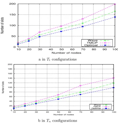
The trend as illustrated in Figure 6 shows that Tt configurations are more greedy in terms
of number of slots to complete convergecast. Balanced routing graphs ensure smaller delays. Indeed, while W ave needs 170 slots to complete convergecast for 100 nodes in Ttconfigurations,
it requires only 118 slots in Tnconfigurations. This result illustrates the good impact of a
traffic-balanced routing tree on the convergecast delays. In Ttconfigurations of 100 nodes, W ave is at
18% from the optimal whereas TMCP is at 42% from the optimal. Moreover, in Tnconfigurations
of 100 nodes, W ave is at 17 % from the optimal whereas TMCP is at 41% from the optimal. This is due to the fact that TMCP partitions the network in disjoint subtrees and schedules all subtrees in parallel, each subtree on a different channel. That is why TMCP requires a number of channels and a number of sink interfaces equal or higher to the number of subtrees. W ave adapts itself to both the number of channels and the number of sink interfaces available.
Notice however that in the comparative performance evaluation, the number of available channels and the number of sink interfaces are always higher than or equal to the number of sink children. In other words, we are always in a favorable context for TMCP.
5.3
Support of additional links
An assumption generally made for the computation of a conflict-free schedule is that there exists no additional links except those in the routing tree. Unfortunately, this does not match real deployments where additional links exist. The existence of additional links is not taken into account in DeT AS and hence may cause collisions: in the same time slot and on the same
0 50 100 150 200 10 20 30 40 50 60 70 80 90 100 Number of slots Number of nodes Wave TMCP Optimal a in Tt configurations 0 20 40 60 80 100 120 140 160 180 200 10 20 30 40 50 60 70 80 90 100 Number of slots Number of nodes Wave TMCP Optimal b in Tn configurations
Figure 6: W ave versus optimal schedule and TMCP: homogeneous traffic
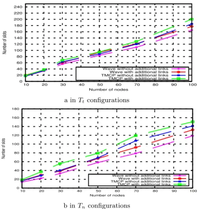
channel frequency, two conflicting transmitters may be scheduled, leading to a collision. This is due to the simple flip-flop schedule adopted, alternating between transmit and receive slots for each active subtree. That is why DeT AS is not suitable in such a case because it fails to ensure deterministic medium access and bounded delays. In T MCP and W ave, additional links are taken into account and conflicts are prevented to occur. A quantitative evaluation is done, where 60% of existing links are added in the routing graph.
Figure 7 depicts the number of slots obtained by T MCP and W ave. The number of slots needed is increased. This happens because additional links create more conflicts. Thus, spatial and frequency reuse is reduced. Nevertheless, the gap between W ave with additional links and W ave without additional links is not large. As illustrated in Figure 7, the number of slots is increased by 8% in Ttconfigurations (respectively 11% in Tn configurations). This is due to our
accurate definition of conflicting nodes detailed in Section 3. In both types of configurations, W ave outperforms T MCP in terms of slots even if additional links exist in the topology. For instance, for 100 nodes, T MCP requires 15.5% (respectively 14%) additional slots compared with W ave in Ttconfigurations (respectively Tnconfigurations), leading to higher data gathering
delays.
5.4
Support of heterogeneous traffic demands
In real data gathering applications, sensor nodes have different sampling rates. Hence, sensor nodes have heterogeneous traffic demands.
0 20 40 60 80 100 120 140 160 180 200 220 240 10 20 30 40 50 60 70 80 90 100 Number of slots Number of nodes
Wave without additional links Wave with additional links TMCP without additional links TMCP with additional links
a in Tt configurations 0 20 40 60 80 100 120 140 160 180 10 20 30 40 50 60 70 80 90 100 Number of slots Number of nodes
Wave without additional links Wave with additional links TMCP without additional links TMCP with additional links
b in Tnconfigurations
Figure 7: Impact of additional links on convergecast schedule length
can be extended to support heterogeneous traffic demands.
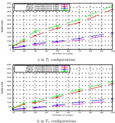
Figure 8 depicts the number of slots obtained by T MCP and W ave, when each sensor node generates a number of packets randomly chosen in the interval [1, 5]. Tnconfigurations, which are
balanced topologies in terms of traffic, require less slots than Ttconfigurations where a subtree
imposes the schedule length. As depicted in Figure 8 heterogeneous traffic results in longer delivery times of packets (because of a higher number of needed slots). Furthermore, we observe the same behavior of curves: W ave outperforms clearly T MCP . Indeed, the difference between W aveand T MCP , in topologies with 100 nodes, is 50 slots in Ttconfigurations (respectively 27
slots in Tn configurations).
5.5
Support of a sink with multiple radio interfaces
Since a sink is a powerful entity in charge of processing data gathered without energy con-straints, it is reasonable to equip it with multiple radio interfaces. In such conditions, the sink equipped with ninterf radio interfaces will be able to receive in parallel from g children, with g = min(ninterf, nchild, nchannel). This increase in communication parallelism will decrease the data gathering delays, as shown by the simulations depicted in Figure 9. In this experiment, the number of channels and the number of radio interfaces of the sink are equal to the number of sink children: this is a favorable context for T MCP .
In Figure 9, a sink, equipped with three radio interfaces, reduces by 6% the convergecast schedule length obtained by W ave in Tt configurations (respectively 13% in Tn configurations)
0 50 100 150 200 250 300 350 400 450 500 550 10 20 30 40 50 60 70 80 90 100 Number of slots Number of nodes Wave: homogeneous traffic Wave: heterogeneous traffic TMCP: homogeneous traffic TMCP: heterogeneous traffic a in Tt configurations 0 50 100 150 200 250 300 350 400 450 500 550 10 20 30 40 50 60 70 80 90 100 Number of slots Number of nodes Wave: homogeneous traffic Wave: heterogeneous traffic TMCP: homogeneous traffic TMCP: heterogeneous traffic
b in Tn configurations
Figure 8: W ave versus TMCP: heterogeneous traffic
time slots only the subtree rooted at the child having the highest number of transmissions. The remaining radio interfaces are kept unused. Paradoxically, in Tn configurations where the traffic
is balanced between all subtrees rooted at the sink children, all the radio interfaces are used simultaneously even in the last time slots.
We can notice also that T MCP provides schedules longer than W ave even when the sink is equipped by multiple radio interfaces. This is because T MCP schedules all nodes in the same subtree on the same channel, unlike W ave.
Authors of DeT AS do not provide any detail how their solution could support multiple radio interfaces for the sink. To the best of our knowledge, we are the first to propose a distributed scheduling algorithm for IEEE 802.15.4e based networks, able to support a sink equipped with multiple radio interfaces.
5.6
Support of different acknowledgment policies
We first compare T MCP , DeT AS and W ave in the absence of acknowledgment. This compari-son shows the merit of W ave in minimizing the data gathering delay. Moreover, some industrial applications robustness requirement. This latter can be met through the immediate acknowledge-ments of packet delivery. Obviously, immediate acknowledgeacknowledge-ments create additional conflicts as was illustrated in Section 3. In this subsection, we assume again that the only existing topology links are those in the routing tree and study the impact of the acknowledgment policy on the number of slots needed.
0 50 100 150 200 250 300 350 400 450 500 550 10 20 30 40 50 60 70 80 90 100 Number of slots Number of nodes Wave TMCP a in Tt configurations 0 50 100 150 200 250 300 350 400 450 500 10 20 30 40 50 60 70 80 90 100 Number of slots Number of nodes Wave TMCP b in Tnconfigurations
Figure 9: Impact of multiple radio interfaces on convergecast schedule length
nodes of a subtree operate on the same channel, the immediate acknowledgment policy will induce a number of conflicts larger than W ave. Indeed, W ave takes advantage of the flexibility of channel selection.
Figure 10 depicts the number of slots obtained by W ave without and with immediate ac-knowledgement. The immediate acknowledgement leads to a higher number of slots. However, the gap between the two curves is tiny (e.g. less than 3% of additional slots). This is due to our accurate conflict definition given in Section 3.
5.7
Support of service differentiation
In a data gathering, we can distinguish several types of traffic: regular traffic for instance cor-responding to periodic sampling and alarm traffic corcor-responding to abnormal situations (e.g. a threshold value is exceeded). To meet the application requirements, the alarm traffic has a higher priority and is transmitted before the regular one. More generally, several classes of traffic can be defined. Each traffic class is associated with a priority and has its own waiting queue. These priorities are taken into account locally in each node for the selection of the next packet to transmit at the MAC level. In the simplest way, classes are ordered by decreasing priority, a packet of class i is scheduled if and only if there is no packet of class j > i waiting to be transmitted. If additional slots are needed to transfer the traffic of class i, node u may take them if allowed by Properties 11 and 12, as shown in Section 6.1. Otherwise, a recomputation of the first wave is done taking into account the new traffic demand.
0 50 100 150 200 10 20 30 40 50 60 70 80 90 100 Number of slots Number of nodes
Wave with ACK Wave without ACK
a in Tt configurations 0 20 40 60 80 100 120 140 160 180 200 10 20 30 40 50 60 70 80 90 100 Number of slots Number of nodes
Wave with ACK Wave without ACK
b in Tn configurations
Figure 10: Impact of acknowledgment policy on convergecast schedule length
its own routing graph. Hence, several routing graphs coexist in the same LLN. This is the object of Section 7.
6
Impact of dynamic changes on the conflict-free schedule
In this section we study the behavior of the W ave algorithm when dynamic changes occur while the conflict-free schedule is orchestrating the medium accesses.
6.1
Impact of retransmissions or changes in application needs
In this subsection, we will show how the scheduling algorithm can adapt to varying traffic de-mands. First, we notice that if the traffic is decreasing, the current schedule is still valid, even if it could be optimized by suppressing slots that have become useless. The problem is how to cope with demands for increasing traffic.
We distinguish two causes for higher traffic demands:
• Since we consider a lossy network, packets may be lost. In the presence of immediate acknowledgment policy, this packet loss is detected by the sender that retransmits its packet. These retransmissions are the first reason why the traffic demand previously done has to be updated.
• Another reason for an update of the traffic demand is due to changes in application re-quirements. For instance, a new traffic is created upon detection of a specific event. This
leads to an increased traffic demand.
In both cases, the conflict-free schedule provided by the scheduling algorithms should take into account these new demands.
Let top subtree(u) denote the subtree rooted at a sink child that contains node u that requires more slots to cope with a change in the application needs.
• With DeT AS, the macroschedule is a juxtaposition in time and/or frequency of microsched-ules, each microschedule schedules a top subtree. The micro-schedule corresponding to the top subtree(u)has to be redone. For the macroschedule, we distinguish two cases:
– if the new microschedule of top subtree(u) is the last one for its channel frequency band in the slotframe, a valid macroschedule is obtained by just replacing the current microschedule of the top subtree(u) by the new one, provided that it does not exceed the slotframe.
– otherwise, the macroschedule has to be computed again.
• With T MCP , authors do not deal with retransmissions or changes in application needs. As T MCP is a centralized solution, a new schedule has to be computed.
• W ave is able to adapt itself to take into account changes in the traffic demand of a node, taking advantage of the following two properties:
Property 11 Any node u 6= sink being assigned slot t in the first wave uses any slot s(t, w) in any wave w with 1 ≤ w ≤ T rans(u). If needed, u may also use any slot s(t, w0) in any wave w0
with T rans(u) < w0≤ M axtrans(t)provided that u transmitted in any wave w00with T rans(u) <
w00< w0. Its parent should be awake in these slots w0. Indeed, for energy efficiency, the parent does not wake up systematically at every wave > T rans(u) but only if its child transmitted in the previous wave > T rans(u).
Proof: Let us focus on the slot t assigned to u in the first wave. The current schedule has taken into account exactly T rans(u) transmissions for u; hence node u uses only the T rans(u) first reproductions of slot t that has been reproduced exactly Maxtrans(t) times. Since the allocation of slots in the first wave takes into account the conflicts between all nodes and since each next wave is an optimized reproduction of the first wave, there is no new conflict introduced by the fact that u transmits in the slots T rans(u) + 1 up to Maxtrans(t). The only limitation is that its parent should be awake.
Property 12 The sink child c being assigned slot t in the first wave and the last slot in the last wave uses any slot s(t, w) in any wave w with 1 ≤ w ≤ T rans(c). If needed, c may also use any slot s(t, w0)in any wave w0with T rans(c) < w0 ≤ Slotf ramelength+T rans(c)−Schedulelength
provided that c transmitted in any wave w00 with T rans(u) < w00< w0. The sink should be awake
in these slots w0.
Proof: The proof is similar to the previous one, except that the schedule of the last slot may be reproduced at the end of the current schedule without compromizing the validity of this new schedule, provided that the slots appended are compatible with the length of the slotframe. Corollary 1 Any node u 6= sink being assigned slot t in the first wave with T rans(u) = M axtrans(t) < maxv6=sinkT rans(v) that requires additional slots leads to a recomputation of
6.2
Impact of a change in the routing graph or in the topology
Let us study the impact of a change in the topology or in the routing graph while the conflict-free schedule is in use. T MCP and DeT AS do not tackle such a change. That is why this subsection is limited to W ave.
We first notice that the breakage of a link taken into account in the computation of the free schedule can never cause collisions. In other words, the schedule remains conflict-free. However, if this link was the link with the preferred parent, a new preferred parent is selected.
If now we focus on the appearance of a new link, this new link may add new conflicting nodes. If these new conflicting nodes were scheduled in the same time slot and on the same channel, collisions will occur. Hence, the schedule must be entirely redone. The following rule summarizes the behavior of W ave.
Rule R5 : With W ave any node u detecting the appearance of a new link with a node v distinguishes two cases
• v is not the new preferred parent of u, u computes its new conflicting nodes applying Property 1 in the absence of acknowledgment and Property 2 in the presence of immediate ackowledgment. Node u checks whether it is scheduled in the same time slot and on the same channel as them. If so, u asks the sink for a recomputation of the first wave, which will be followed by a local computation on all nodes of the next waves. Otherwise, the current schedule is kept.
• v is the new preferred parent of u, W ave must recompute the first wave and then each node will locally compute the slots granted to itself and its children in the next waves.
7
Support of multiple routing graphs
In this section, we study the coexistence of several routing graphs in the same LLN. Two routing graphs RG1 and RG2 are said independent if and only if no node of RG1 conflicts with a node of RG2.
Property 13 Two routing graphs RG1 and RG2 are not independent if and only if there is a common node belonging to both RG1 and RG2 or there is a common link between a node of RG1 and a node of RG2.
Proof: We first prove that two routing graphs RG1 and RG2 are not independent if and only if there exists a path of length h, with 0 ≤ h ≤ 1 between them. We proceed by contradiction, if there exists no path between the two routing graphs, no node of RG1 would conflict with a node of RG2. Hence the two routing graphs are independent. Consequently, there is a path between them. Let h be the length of this path and let us assume h ≥ 2. In the presence of immediate acknowledgment, it is not possible to find a conflict between a node of RG1 and a node of RG2 using the conflicts described in Property 2. Similarly, in the absence of immediate acknowledgment, it is not possible to find a conflict between a node of RG1 and a node of RG2 using the conflicts described in Property 1. Hence h < 2.
It follows that there exists a path of length h ≤ 1. If h = 0: there is a common node belonging to both RG1 and RG2. If h = 1: there is a common link between a node of RG1 and a node of RG2.
Since the sink is in charge of triggering the schedule of its routing graph RG, it must know whether RG is dependent on any other routing graph. That is why Rule R6 is applied.
Rule R6 : Any node belonging to any routing graph RG1 that also belongs to a routing graph RG2 sends a message to the sink of RG1 as well as the sink of RG2. Similarly, any node belonging to any routing graph RG that has a link to a node in another routing graph sends a message to the sink of RG.
In the following, we distinguish two cases: the routing graphs are independent or not.
7.1
Independent routing graphs
Two independent routing graphs can be scheduled independently. Their schedule is always conflict-free.
Property 14 If the coexisting routing graphs are all independent two-to-two, they can share the same time slots and frequencies. The number of slots needed to schedule these routing graphs is equal to the maximum of the number of slots needed by each of them taken separately. The number of channels is equal to the maximum of channels needed by each of them taken separately. Figure 11 depicts a frameslot scheduling three routing graphs RG1, RG2 and RG3. These routing graphs are independent two-by-two. Consequently, they are all scheduled on the same channel frequencies and in the same time slots. The number of slots needed to schedule them all is equal to 5, which is also the number of slots needed to schedule RG1 alone.
Figure 11: Schedule of independent routing graphs.
7.2
Dependent routing graphs
If the coexisting routing graphs are not independent, they cannot be scheduled independently: collisions may occur during data gathering. These collisions will prevent either a receiving node to correctly receive a data packet destinated to it, or a transmitting node to correctly receive the acknowledgment of its data packet. Hence, such collisions must be avoided to ensure the quality of service required by data gathering.
To prevent the occurrence of conflicts at runtime, W ave uses a coarse granularity approach.
7.2.1 General principles
This approach prevents conflicts to occur at a coarse granularity level by applying first Rule R7 and then Rule R8:
Rule R7 : If there exists at least one node belonging to two routing graphs RG1 and RG2, then these routing graphs should be scheduled in different time slots (i.e. time exclusion).
Rule R8 : If there exists at least one link between a node of routing graph RG1 and a node of routing graph RG2, then these routing graphs should be scheduled on different frequencies (i.e. channel frequency exclusion). If this is impossible, then they are scheduled in different time