HAL Id: hal-01398867
https://hal.inria.fr/hal-01398867
Submitted on 17 Nov 2016
HAL is a multi-disciplinary open access
archive for the deposit and dissemination of
sci-entific research documents, whether they are
pub-lished or not. The documents may come from
teaching and research institutions in France or
abroad, or from public or private research centers.
L’archive ouverte pluridisciplinaire HAL, est
destinée au dépôt et à la diffusion de documents
scientifiques de niveau recherche, publiés ou non,
émanant des établissements d’enseignement et de
recherche français ou étrangers, des laboratoires
publics ou privés.
Deriving reproducible biomarkers from multi-site
resting-state data: An Autism-based example
Alexandre Abraham, Michael Milham, Adriana Di Martino, R. Cameron
Craddock, Dimitris Samaras, Bertrand Thirion, Gaël Varoquaux
To cite this version:
Alexandre Abraham, Michael Milham, Adriana Di Martino, R. Cameron Craddock, Dimitris Samaras,
et al.. Deriving reproducible biomarkers from multi-site resting-state data: An Autism-based example.
NeuroImage, Elsevier, 2016, �10.1016/j.neuroimage.2016.10.045�. �hal-01398867�
Deriving reproducible biomarkers from multi-site resting-state data: An
Autism-based example
Alexandre Abrahama,b,∗
, Michael Milhame,f
, Adriana Di Martinog
, R. Cameron Craddocke,f, Dimitris Samarasc,d, Bertrand Thiriona,b, Gael Varoquauxa,b
aParietal Team, INRIA Saclay-ˆIle-de-France, Saclay, France
bCEA, DSV, I2BM, Neurospin bˆat 145, 91191 Gif-Sur-Yvette, France
cStony Brook University, NY 11794, USA
dEcole Centrale, 92290 Chˆatenay Malabry, France
eChild Mind Institute, New York, USA
fNathan S. Kline Institute for Psychiatric Research, Orangeburg, New York, USA
gNYU Langone Medical Center, New York, USA
Abstract
Resting-state functional Magnetic Resonance Imaging (R-fMRI) holds the promise to reveal functional biomarkers of neuropsychiatric disorders. However, extracting such biomarkers is challenging for complex multi-faceted neuropatholo-gies, such as autism spectrum disorders. Large multi-site datasets increase sample sizes to compensate for this complexity, at the cost of uncontrolled heterogeneity. This heterogeneity raises new challenges, akin to those face in realistic di-agnostic applications. Here, we demonstrate the feasibility of inter-site classification of neuropsychiatric status, with an application to the Autism Brain Imaging Data Exchange (ABIDE) database, a large (N=871) multi-site autism dataset. For this purpose, we investigate pipelines that extract the most predictive biomarkers from the data. These R-fMRI pipelines build participant-specific connectomes from functionally-defined brain areas. Connectomes are then compared across participants to learn patterns of connectivity that differentiate typical controls from individuals with autism. We predict this neuropsychiatric status for participants from the same acquisition sites or different, unseen, ones. Good choices of methods for the various steps of the pipeline lead to 67% prediction accuracy on the full ABIDE data, which is significantly better than previously reported results. We perform extensive validation on multiple subsets of the data defined by different inclusion criteria. These enables detailed analysis of the factors contributing to successful connectome-based prediction. First, prediction accuracy improves as we include more subjects, up to the maximum amount of subjects available. Second, the definition of functional brain areas is of paramount importance for biomarker discovery: brain areas extracted from large R-fMRI datasets outperform reference atlases in the classification tasks. Keywords: data heterogeneity, resting-state fMRI, data pipelines, biomarkers, connectome, autism spectrum disorders
1. Introduction
In psychiatry, as in other fields of medicine, both the standardized observation of signs, as well as the symptom profile are critical for diagnosis. However, compared to other fields of medicine, psychiatry lacks accompanying objective markers that could lead to more refined diag-noses and targeted treatment [1]. Advances in non-invasive brain imaging techniques and analyses (e. g. [2, 3]) are showing great promise for uncovering patterns of brain structure and function that can be used as objective mea-sures of mental illness. Such neurophenotypes are impor-tant for clinical applications such as disease staging, deter-mination of risk prognosis, prediction and monitoring of treatment response, and aid towards diagnosis (e. g. [4]).
∗Corresponding author
Email address: [email protected] (Alexandre Abraham)
Among the many imaging techniques available, resting-state fMRI (R-fMRI) is a promising candidate to define functional neurophenotypes [5,3]. In particular, it is non-invasive and, unlike conventional task-based fMRI, it does not require a constrained experimental setup nor the ac-tive and focused participation of the subject. It has been proven to capture interactions between brain regions that may lead to neuropathology diagnostic biomarkers [6]. Nu-merous studies have linked variations in brain functional architecture measured from R-fMRI to behavioral traits and mental health conditions such as Alzheimer disease (e. g. [7, 8], Schizophrenia (e. g. [9, 10, 11, 12]), ADHD, autism (e. g. [13]) and others (e. g. [14]). Extending these findings, predictive modeling approaches have re-vealed patterns of brain functional connectivity that could serve as biomarkers for classifying depression (e. g. [15]), ADHD (e. g. [16]), autism (e. g. [17]), and even age [18]. This growing number of studies has shown the feasibility of using R-fMRI to identify biomarkers. However questions
about the readiness of R-fMRI to detect clinically useful biomarkers remain [13]. In particular, the reproducibility and generalizability of these approaches in research or clin-ical settings are debatable. Given the modest sample size of most R-fMRI studies, the effect of cross-study differ-ences in data acquisition, image processing, and sampling strategies [19,20,21] has not been quantified.
Using larger datasets is commonly cited as a solu-tion to challenges in reproducibility and statistical power [22]. They are considered a prerequisite to R-fMRI-based classifiers for the detection of psychiatric illness. Recent efforts have accelerated the generation of large databases through sharing and aggregating independent data samples[23, 24,25]. However, a number of concerns must be addressed before accepting the utility of this ap-proach. Most notably, the many potential sources of un-controlled variation that can exist across studies and sites, which range from MRI acquisition protocols (e. g. scanner type, imaging sequence, see [26]), to participant instruc-tions (e. g. eyes open vs. closed, see [27]), to recruitment strategies (age-group, IQ-range, level of impairment, treat-ment history and acceptable comorbidities). Such varia-tion in aggregate samples is often viewed as dissuasive, as its effect on diagnosis and biomarker extraction is un-known. It commonly motivates researchers to limit the number of sites included in their analyses at the cost of sample size.
Cross-validated results obtained from predictive mod-els are more robust to inhomogeneities: they measure model generalizability by applying it to unseen data, i. e., data not used to train the model. In particular, leave-out cross-validation strategies, which remove single individuals (or random subsets), are common in biomarkers studies. However, these strategies do not measure the effect of po-tential site-specific confounds. In the present study we leverage aggregated R-fMRI samples to address this prob-lem. Instead of leaving out random subsamples as test sets, we left out entire sites to measure performance in the presence of uncontrolled variability.
Beyond challenges due to inter-site data heterogene-ity, choices in the functional-connectivity data-processing pipeline further add to the variability of results [28,27,29]. While preprocessing procedures are now standard, the dif-ferent steps of the prediction pipeline vary from one study to another. These entail specifying regions of interest, ex-tracting regional time courses, computing connectivity be-tween regions, and identifying connections that relate to subject’s phenotypes [15,30,31,32].
Lack of ground truth for brain functional architec-ture undermines the validation of R-fMRI data-processing pipelines. The use of functional connectivity for individ-ual prediction suggests a natural figure of merit: prediction accuracy. We contribute quantitative evaluations, to help settling down on a parameter-free pipeline for R-fMRI. Using efficient implementations, we were able to evaluate many pipeline options and select the best method to es-timate atlases, extract connectivity matrices, and predict
phenotypes.
To demonstrate that pipelines to extract R-fMRI neuro-phenotypes can reliably learn inter-site biomark-ers of psychiatric status on inhomogeneous data, we ana-lyzed R-fMRI in the Autism Brain Imaging Data Exchange (ABIDE) [25]. It compiles a dataset of 1112 R-fMRI par-ticipants by gathering data from 17 different sites. Af-ter preprocessing, we selected 871 to meet quality criAf-teria for MRI and phenotypic information. Our inter-site pre-diction methodology reproduced conditions found under most clinical settings, by leaving out whole sites and using them as newly seen test sets. To validate the robustness of our approach, we performed nested cross-validation and varied samples per inclusion criteria (e. g. sex, age). Fi-nally, to assess losses in predictive power associated with using a heterogeneous aggregate dataset instead of uni-formly defined samples, we included a comparison of intra-and inter-site prediction strategies.
2. Material and methods
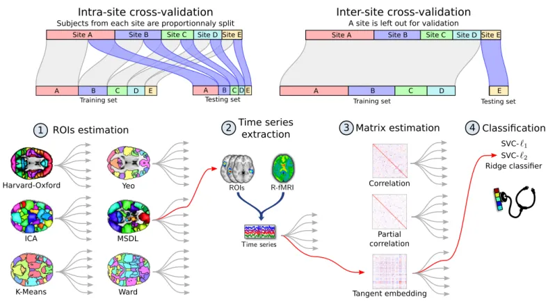
A connectome is a functional-connectivity matrix be-tween a set brain regions of interest (ROIs). We call such a set of ROIs an atlas, even though some of the methods we consider extract the regions from the data rather than relying on a reference atlas (seeFigure 1). We investigate here pipelines that discriminate individuals based on the connection strength of this connectome [33], with a classi-fier on the edge weights [15].
Specifically, we consider connectome-extraction pipelines composed of four steps: 1) region estimation, 2) time series extraction, 3) matrix estimation, and 4) classification –see Figure 1. We investigate different options for the various steps: brain parcellation method, connectivity matrix estimation, and final classifier.
In order to measure the impact of uncontrolled vari-ability on prediction performance, we designed a diagnosis task where the model classifies participants coming from an acquisition site not seen during training.
2.1. Datasets: Preprocessing and Quality Assurance (QA) We ran our analyses on the ABIDE repository [25], a sample aggregated across 17 independent sites. Since there was no prior coordination between sites, the scan and diagnostic/assessment protocols vary across sites 1.
To easily replicate and extend our work, we rely on a pub-licly available preprocessed version of this dataset provided by the Preprocessed Connectome Project2 initiative. We
specifically used the data processed with the Configurable Pipeline for the Analysis of Connectomes [34] (C-PAC). Data were selected based on the results of quality visual in-spection by three human experts who inspected for largely
1See http://fcon_1000.projects.nitrc.org/indi/abide/ for specific information
Training set Testing set
A B C D E A B C D E
Training set Testing set
ROIs estimation
Harvard-Oxford Yeo
ICA MSDL
K-Means Ward
Time series
extraction Matrix estimation
Correlation Partial correlation Tangent embedding Classification Ridge classifier SVC-Intra-site cross-validation
Subjects from each site are proportionnaly split
R-fMRI ROIs
Time series
4
1 2 3
Site A Site B Site C Site D Site E Site A Site B Site C Site D Site E
A B C D E
Inter-site cross-validation A site is left out for validation
Figure 1: Functional MRI analysis pipeline. Cross-validation schemes used to validate the pipeline are presented above. Intra-site cross-validation consists of randomly splitting the participants into training and testing sets while preserving the ratio of samples for each site and condition. Inter-site cross-validation consists of leaving out participants from an entire site as testing set. In the first step of the pipeline, regions of interest are estimated from the training set. The second step consists of extracting signals of interest from all the participants, which are turned into connectivity features via covariance estimation at the third step. These features are used in the fourth step to perform a supervised learning task and yield an accuracy score. An example of pipeline is highlighted in red. This pipeline is the one that gives best results for inter-site prediction. Each model is decribed in the section relative to material and methods.
incomplete brain coverage, high movement peaks, ghost-ing and other scanner artifacts. This yielded 871 subjects out of the initial 1112.
Preprocessing included slice-timing correction, image realignment to correct for motion, and intensity normaliza-tion. Nuisance regression was performed to remove signal fluctuations induced by head motion, respiration, cardiac pulsation, and scanner drift [35, 36]. Head motion was modeled using 24 regressors derived from the parameters estimated during motion realignment [37], scanner drift was modeled using a quadratic and linear term, and phys-iological noise was modeled using the 5 principal compo-nents with highest variance from a decomposition of white matter and CSF voxel time series (CompCor) [38]. Af-ter regression of nuisance signals, fMRI was coregisAf-tered on the anatomical image with FSL BBreg, and the results where normalized to MNI space with the non-linear regis-tration from ANTS [39]. Following time series extraction, data were detrended and standardized (dividing by the standard deviation in each voxel).
2.2. Step 1: Region definition
To reduce the dimensionality of the estimated connec-tomes, and to improve the interpretability of results, con-nectome nodes were defined from regions of interest (ROIs)
rather than single voxels. ROIs can be either selected from a priori atlases or directly estimated from the correlation structure of the data being analyzed. Several choices for both approaches were used and compared to evaluate the impact of ROI definition on prediction accuracy. Note that the ROI were all defined on the training set to avoid possible overfitting.
We considered the following predefined atlases: Har-vard Oxford [40], a structural atlas computed from 36 individuals’ T1 images, Yeo [41], a functional atlas com-posed of 17 networks derived from clustering [42] of func-tional connectivity on a thousand individuals, and Crad-dock [43], a multiscale functional atlas computed using constrained spectral clustering, to study the impact of the number of regions.
We derived data-driven atlases based on four strate-gies. We explored two clustering methods: K-Means, a technique to cluster fMRI time series [44, 45], which is a top-down approach minimizing cluster-level variance; and Ward’s clustering, which also minimizes a variance cri-terion using hierarchical agglomeration. Ward’s algorithm admits spatial constraints at no cost and has been exten-sively used to learn brain parcellations [45]. We also ex-plored two decomposition methods: Independent com-ponent analysis (ICA) and multi-subject dictionary
learning (MSDL). ICA is a widely-used method for ex-tracting brain maps from R-fMRI [46,47] that maximizes the statistical independence between spatial maps. We specifically used the ICA implementation of [48]. MSDL extracts a group atlas based on dictionary learning and multi-subject modeling, and employs spatial penalization to promote contiguous regions [49]. Unlike MSDL and Ward clustering, ICA and K-Means do not take into ac-count the spatial structure of the features and are not able to enforce a particular spatial constraint on their compo-nents. We indirectly provide such structure by applying a Gaussian smoothing on the data [45] with a full-width half maximum varying from 4mm to 12mm. Differences in the number of ROIs in the various atlases present a poten-tial confound for our comparisons. As such, connectomes were constructed using only the 84 largest ROIs from each atlas, following [49]3.
2.3. Step 2: Time-series extraction
The common procedure to extract one representative time series per ROI is to take the average of the voxel signals in each region (for non overlapping ROIs) or the weighted average of non-overlapping regions (for fuzzy maps). For example, ICA and MSDL produce overlapping fuzzy maps. Each voxel’s intensity reflects the level of con-fidence that this voxel belongs to a specific region in the atlas. In this case, we found that extracting time courses using a spatial regression that models each volume of R-fMRI data as a mixture of spatial patterns gives better results (details in Appendix A and Figure A3). For non-overlapping ROIs, this procedure is equivalent to weighted averaging on the ROI maps.
After this extraction, we remove at the region level the same nuisance regressors as at the voxel level in the preprocessing. Signals summarizing high-variance voxels (CompCor [38]) are regressed out: the 5 first principal components of the 2% voxels with highest variance. In addition, we extract the signals of ROIs corresponding to physiological or acquisition noise4and regress them out to reject non-neural information [33]. Finally, we also regress out primary and secondary head motion artifacts using 24-regressors derived from the parameters estimated during motion realignment [37].
2.4. Step 3: Connectivity matrix estimation
Since scans in the ABIDE dataset do not include enough R-fMRI time points to reliably estimate the true
3For Harvard-Oxford and Yeo reference atlases, selecting 84 ROIs
yields slightly better results than using the full version as shown in Figure A2. This is probably due to the fact that these additional regions are smaller and less important regions, hence they induce spurious correlations in the connectivity matrices.
4We identify these ROIs using an approach similar to FSL FIX
(FMRIB’s ICA-based Xnoiseifier). FIX extracts spatial and tempo-ral descriptors from matrix decomposition results and uses a clas-sifier trained on manually labeled components to determine if they correspond to noise.
covariance matrix for a given individual, we used the Ledoit-Wolf shrinkage estimator, a parameter-free regu-larized covariance estimator [50], to estimate relationships between ROI time series (details are given in Appendix B). For pipeline step 3, we studied three different con-nectivity measures to capture interactions between brain regions: i) the correlation itself, ii) partial correlations from the inverse covariance matrix [33, 51], and iii) the tangent embedding parameterization of the covariance ma-trix [48,52]. We obtained one connectivity weight per pair of regions for each subject. At the group level, we ran a nuisance regression across the connectivity coefficients to remove the effects of site, age and gender.
2.5. Step 4: Supervised learning
As ABIDE represents a post-hoc aggregation of data from several different sites, the assessments used to mea-sure autism severity vary somewhat across sites. As a con-sequence, autism severity scores are not directly quantita-tively comparable between sites. However, the diagnosis between ASD and Typical Control (TC) is more reliable and has already been used in the context of classification [53,13,54].
Discriminating between ASD and TC individuals is a supervised-learning task. We use the connectivity mea-sures between all pairs of regions, extracted in the previ-ous step, as features to train a classifier across individuals to discriminate ASD patients from TC.
We explore different machine-learning methods5. We
first rely on the most commonly used approach, the `2 -penalized support vector classification SVC. Given that we expect only a few connections to be important for di-agnosis, we also include the `1-penalized sparse SVC. Fi-nally, we include ridge regression, which also uses an `2 penality but is faster than the SVC. For all models we use the implementation of the scikit-learn library [55]6.
We chose to work only with linear models for their inter-pretability. In particular, insubsection 3.7we inspect clas-sifier weights to identify which connections are the most important for prediction.
2.6. Exploring dataset heterogeneity
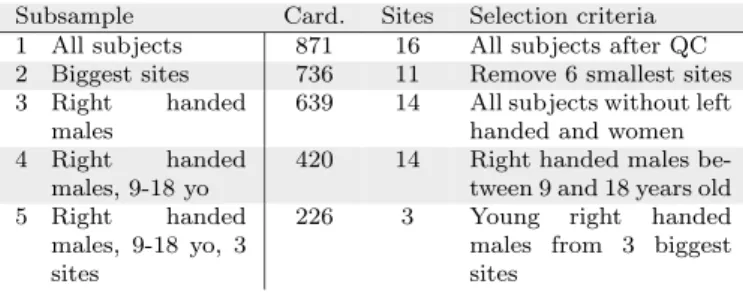
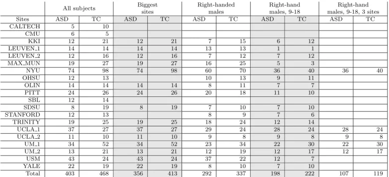
Previous studies of prediction using the ABIDE sam-ple [13, 54] have included less than 25% of the available data, most likely to limit heterogeneity – not only due to differences in imaging, but also to factors such as age, sex, and handedness. We explored the effect of such choice on the results, by examining data subsets of different hetero-geneity (see Table 1). These included: subsample #1
-5For the sake of simplicity, we report only the 3 main methods
here. However, we also investigated random forests and Gaussian naive Bayes, that gave low prediction performance. Feature selection also led to worse results, both with univariate ANOVA screening and
with sparse models such as Lasso or SVC-`1–see FigureA4for more
details. Logistic regression gave results similar to SVC.
6Software versions: python 2.7, scikit-learn 0.17.1, scipy 0.14.0,
Subsample Card. Sites Selection criteria
1 All subjects 871 16 All subjects after QC
2 Biggest sites 736 11 Remove 6 smallest sites
3 Right handed
males
639 14 All subjects without left
handed and women
4 Right handed
males, 9-18 yo
420 14 Right handed males
be-tween 9 and 18 years old
5 Right handed
males, 9-18 yo, 3 sites
226 3 Young right handed
males from 3 biggest sites
Table 1: Subsets of ABIDE used in evaluation. We explore sev-eral subsets of ABIDE with different homogeneity. Card. stands for the cardinality of the dataset, i. e. the number of subjects. More de-tails about these subsets are presented in the appendices –Table A2.
all participants (871 individuals, 727 males and 144 fe-males, 6 to 64 years old) is the full set of individuals that passed QA, subsample #2 - largest sites (736 individ-uals, 613 males and 123 females) 6 sites with less than 30 participants are removed from subsample #1, subsam-ple #3 - right handed males (639 individuals) consists of the right-handed males from subsample #1, subsample #4 - right handed males, 9-18 years (420 individuals) is the restriction of subsample #3 to participants between 9 and 18 years old; subsample #5 - right handed males, 9-18 yo, 3 sites (226 individuals) are the individuals from subsample #4 belonging to the three largest sites (see Ta-ble A2for more details)7.
2.7. Experiments: prediction on heterogeneous data ABIDE datasets come from 17 international sites with no prior coordination, which is a typical clinical applica-tion setting. In this setting, we want to: i) measure the performance of different prediction pipelines, ii) use these measures to find the best options for each pipeline step (Figure 1) and, iii) extract ASD biomarkers from the best pipeline.
Cross-validation. In order to measure the prediction ac-curacy of a pipeline, we use 10-fold cross-validation by training it exclusively on training data (including atlas es-timation) and predicting on the testing set. Any hyper-parameter of the various methods used inside a pipeline is set internally in a nested cross-validation.
We used two validation approaches. Inter-site pre-diction addresses the challenges associated with aggregate datasets by using whole sites as testing sets. This scenario also closely simulates the real world clinical challenge of not being able to sample data from every possible site. Note that this cross-validation can only be applied on a dataset with at least 10 acquisition sites, in order to leave out a different site in each fold. We do not apply it on sub-sample #5 that has been restricted to 3 sites to reduce site-specific variability. Intra-site prediction builds training
7Table A6lists subjects of each subsample. The lists of subjects
for each cross-validation fold are available athttps://team.inria.
fr/parietal/files/2016/04/cv_abide.zip
and testing sets are as homogeneous as possible, reduc-ing site-related variability. It is based on stratified shuffle split cross-validation, which splits participants into train-ing and test sets while preservtrain-ing the ratio of samples for each site and condition. We used 80% of the dataset for training and the remaining for testing.
Learning curves. A learning curve measures the impact of the number of training samples on the performance of a predictive model. For a given prediction task, the learn-ing curve is constructed by varylearn-ing the number of samples in the training set with a constant test set. Typically, an increasing curve indicates that the model can still gain ad-ditional useful information from more data. It is expected that the performance of a model will plateau at some point. Summarizing prediction scores for a pipeline choice. To quantify the impact of the different options on the predic-tion accuracy, we select representative predicpredic-tion scores for each model. Indeed, for ICA, K-Means, and MSDL, we ex-plore several values for each parameters and thus obtain a range of prediction values. For these methods, we use the 10% best-performing pipelines for post-hoc analysis
8. We do not rely only on the top-performing pipelines,
as they may result from overfitting, nor the complete set of pipelines as some pipelines yield bad scores because of bad parametrization and may artificially lower the perfor-mance of these methods.
Impact of pipeline choices on prediction accuracy. In or-der to determine the best pipeline option at each step, we want to measure the impact of these choices on the predic-tion scores. In a full-factorial ANOVA, we then fit a linear model to explain prediction accuracy from the choice of pipeline steps, modeled as categorical variables. We re-port the corresponding effect size and its 95% confidence interval.
Pairwise comparison of pipeline choice. Two options can also be compared by comparing the scores between pairs of pipelines that differ only by that option using a Wilcoxon test that does not rely on Gaussian assumptions.
Extracting biomarkers. For a given pipeline, the final clas-sifier yields a biomarker to diagnose between HC and ASD. To characterize this biomarker, we measure p-values on the classifier weights. We obtain the null distribution of the weights by permuting the prediction labels.
8Note that the criterion used to select the data-point used for
the post-hoc analysis, i. e. the 10% best performing, is independent from the factors studied in this analysis, as we select the 10% best
performing for each value of these factors. Hence, the danger of
inflating effects by a selection [56] does not apply to the post hoc analysis.
2.8. Computational aspects
For data-driven brain atlas models (e. g. ICA), region-extraction methods entail feature learning on up to 300 GB of data, too big to fit in memory. Systematic study requires many cross-validations and subsamples and thus careful computational optimizations. Hence, for K-Means and ICA, we reduced the length of the time series by apply-ing PCA dimensionality reduction with efficient random-ized SVD [57]. MSDL uses algorithmic optimizations [49] to process a large number of subjects in a reasonable time
9 (2 hours for 871 subjects). However, it is still the most
costly method because of the number of runs required to find the optimal value for its 3 parameters.
For reproducibility, we rely on the publicly available implementations of the scikit-learn package [55] for all the clustering algorithms, connectivity matrix estimators and predictors.
3. Results
Here we present the most notable trends emerging from our analyses. More details are provided in supplementary materials. First, we compared inter- and intra-site predic-tion of ASD diagnostic labels while varying the number of subjects in the training set. Second, in a post-hoc anal-ysis, we identified the pipeline choices most relevant for prediction and proposed a good choice of pipeline steps for prediction. Finally, by analyzing the weights of the classifiers, we highlighted functional connections that best discriminate between ASD and TC.
3.1. Overall prediction results
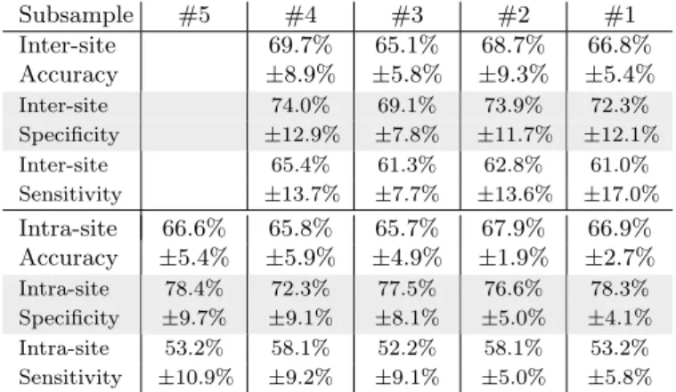
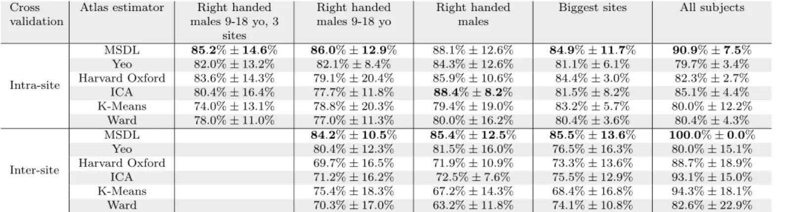
For inter-site prediction, the highest accuracy obtained on the whole dataset is 66.8% (see Table 2) which ex-ceeds previously published ABIDE findings [53,13,54] and chance at 53.7%10. Importantly, performance increases
steadily with training set size, for all subsamples (Figures2 and A6). This increase implies that optimal classification performance is not reached even for the largest dataset tested.
The main difference between intra-site and inter-site settings is that the variability of inter-site prediction is higher (Table 2). However, this difference disappears with a large enough training set (Figure 2). This is encouraging for clinical applications.
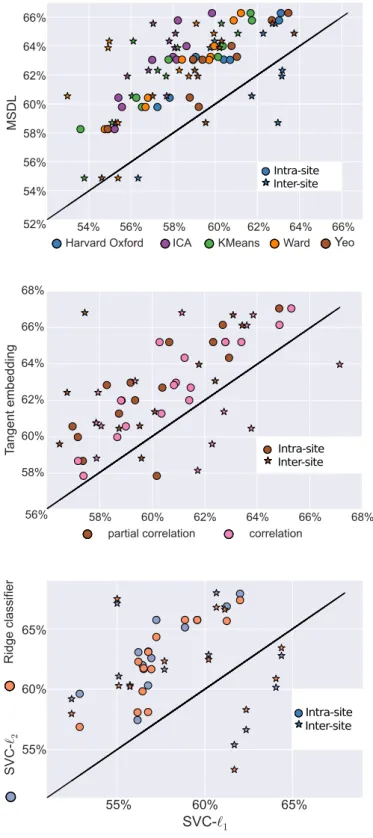
As shown in Figure 3, the best predicting pipeline is MSDL, tangent space embedding and l2-regularized classi-fiers (SVC-l2 and ridge classifier). All effects are observed
9Despite the optimizations, the whole study presented here is very
computationally costly. Indeed, the nested cross-validation, the vari-ous pipeline options, and the varivari-ous subsets, would lead to a compu-tation time of 10 years on a computer with 8 cores and 32GB RAM. We used a computer grid to reduce it to two months.
10Chance is calculated by taking the highest score obtained by a
dummy classifier that predicts random labels following the distribu-tion of the two classes.
Subsample #5 #4 #3 #2 #1 Inter-site 69.7% 65.1% 68.7% 66.8% Accuracy ±8.9% ±5.8% ±9.3% ±5.4% Inter-site 74.0% 69.1% 73.9% 72.3% Specificity ±12.9% ±7.8% ±11.7% ±12.1% Inter-site 65.4% 61.3% 62.8% 61.0% Sensitivity ±13.7% ±7.7% ±13.6% ±17.0% Intra-site 66.6% 65.8% 65.7% 67.9% 66.9% Accuracy ±5.4% ±5.9% ±4.9% ±1.9% ±2.7% Intra-site 78.4% 72.3% 77.5% 76.6% 78.3% Specificity ±9.7% ±9.1% ±8.1% ±5.0% ±4.1% Intra-site 53.2% 58.1% 52.2% 58.1% 53.2% Sensitivity ±10.9% ±9.2% ±9.1% ±5.0% ±5.8%
Table 2: Average accuracy, specificity and sensitivity
sco-res (and standard deviation) for top performing pipelines. Accuracy is the fraction of well-classified individuals (chance level is at 53.7%). Specificity is the fraction of well classified healthy indi-viduals among all healthy indiindi-viduals (percentage of well-classified
negatives). Sensitivity is the ratio of ASD individuals among all
subjects classified as ASD (percentage of positives that are true pos-itives). Results per atlas are available in the appendices –Table A5.
0.1 0.2 0.3 0.4 0.5 0.6 0.7 0.8 0.9 1.0
Ratio of training set used
50%
52%
54%
56%
57%
60%
62%
64%
66%
Mean accuracy over 10 folds
Intra-site
Inter-site
Figure 2: Learning curve. Classification results obtained by vary-ing the ratio of the trainvary-ing set usvary-ing to train the classifier while keeping a fixed testing set. The colored bands represent the stan-dard error of the prediction. A score increasing with the number of subjects, i. e. a positive slope indicates that the addition of new sub-jects improves performance. This curve is an average of the results obtained on several subsamples. Detailed results per subsamples are presented in the appendices –Figure A6
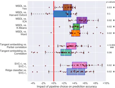
with p < 0.01. Detailed pairwise comparisons (Figure 4) confirm these trends by showing the effect of each option compared to the best ones. Results of intra-site prediction have smaller standard error, confirming higher variability of inter-site prediction results (Figure A5).
3.2. Effect of the choice of atlas
The choice of atlas appears to have the greatest im-pact on prediction accuracy (Figure 3). Estimation of an atlas from the data with MSDL, or using reference at-lases leads to maximal performance. Of note, for smaller samples, data-driven atlas-extraction methods other than MSDL perform poorly (Figure A8). In this regime, noise
Cross validation scheme ABIDE subsample Step 1: Atlas extraction Step 3: Covariance matrix Step 4: Predictor
Figure 3: Impact of pipeline steps on prediction. Each block of bars represents a step of the pipeline (namely step 1, 3 and 4). We also prepended two steps corresponding to the cross-validation schemes and ABIDE subsamples. Each bar represents the impact of the corresponding option on the prediction accuracy, relative to the mean prediction. This effect is measured via a full-factorial analysis of variance (ANOVA), analyzing the contribution of each step in a linear model. Each step of the pipeline is considered as a categorical variable. Error bars give the 95% confidence interval. Multi Subject Dictionary Learning (MSDL) atlas extraction method gives signifi-cantly better results while reference atlases are slightly better than the mean. Among all matrix types, tangent embedding is the best on
all ABIDE subsets. Finally, l2-regularized classifiers perform better
than l1-regularized ones. Results for each subsamples are presented in the appendices –Figure A8.
can be problematic and limit the generalizability of atlases derived from data.
MSDL performs well regardless of sample size, and the performance gain is significant compared to all other strategies apart from the Harvard-Oxford atlas (Figure 4). This is likely attributable to MSDL’s strong spatially-structured regularization that increases its robustness to noise.
3.3. Effect of the covariance matrix estimator
While correlation and partial correlation approaches are currently the two dominant approaches to connectome estimation in the current R-fMRI literature, our results highlight the value of tangent-space projection that out-performs the other approaches in all settings (Figure 3and Figure 4), though the difference is significant only com-pared with correlation matrices (Figure 4). This gain in prediction accuracy is not without a cost, as the matri-ces derived cannot be read as correlation matrimatri-ces. Yet,
0.02* 0.02* 0.1 0.03* 0.02* < 0.001 * * 0.06 0.02* 0.02* p-values
Figure 4: Comparison of pipeline options. Each plot compares the classification accuracy scores if one parameter is changed and the others kept fixed. We measured statistical signficance using a Wilcoxon signed rank test and corrected for multiple comparisons. Detailed one-to-one comparison of the scores are shown in the ap-pendices –Figure A5
the differences in connectivity that they capture can be directly interpreted [58].
Among the correlation-based approaches, full correla-tions outperformed partial correlacorrela-tions, most notably for intra-site prediction. These limitations of partial corre-lations may reflect estimation challenges11 with the
rela-tively short time series included in ABIDE datasets (typ-ically 5-6 minutes per participant).
3.4. Effect of the final classifier
The results show that `2-regularized classifiers perform best in all settings (Figure 3and Figure 4). This may be due to the fact that a global hypoconnectivity, as previ-ously observed in ASD patients, is not well captured by `1-regularized classifiers, which induce sparsity. In addi-tion `2-penalization is rotationally-invariant, which means that it is not sensitive to an arbitrary mixing of features. Such mixing may happen if a functional brain module sits astride several regions. Thus, a possible explanation for the good performance of `2-penalization is that it does not need an optimal choice of regions, perfectly aligned with the underlying functional modules.
3.5. Effect of the dataset size and heterogeneity
While not a property of the data-processing pipeline itself, a large number of training subjects is the most im-portant factor of success for prediction. Indeed, we ob-serve that prediction results improve with the number of subjects, even for large number of subjects (Figure 3).
11Note that we experimented with a variety of more sophisticated
covariance estimators, including GraphLasso, though without im-proved results.
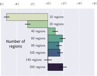
Number of regions
Figure 5: Impact of the number of regions on prediction: each bar indicates the impact of the number of regions on the prediction accuracy relative to the mean of the prediction. These values are coefficients in a linear model explaining the best classification sco-res as function of the number of regions. Error bars give the 95% confidence interval, computed by a full factorial ANOVA. Atlases containing more than 40 ROIs give better results in all settings. Re-sults per subsamples are presented in the appendices –Figure A9.
Despite that increase, we note that prediction on the largest subsample (subsample #1) gives lower scores than prediction on subsample #2, which may be due to the vari-ance introduced by small sites. We also note that the im-portance of the choice between each option of the pipeline decreases with the number of subjects (Figure A8). 3.6. Effect of the number of regions
In order to compare models of similar complexity, the previous experiments were restricted to 84 regions as in [49]. However, this choice is based on previous studies and may not be the optimal choice for our problem. To validate this aspect of the study, we also varied the num-ber of regions and analyzed its impact on the classifica-tion results in Figure 5, similarly to Figure 3. In order to avoid computational cost12, we explored only two
at-lases: the data-driven Ward’s hierarchical clustering and spectral clustering atlases computed in [43].
Across all settings, we distinguish 3 different regimes. First, below 20 ROIs, performance is bad. Indeed very large regions average out signals of different functional ar-eas. Above 140 ROIs, the results seem to be unstable, though this trend is less clear in intra-site prediction. Fi-nally, the best results are between 40 and 100 ROIs. Our choice of 84 ROIs is within the range of best performing models.
12As MSDL is much more computationally expensive than Ward,
we have not explored the effect of modifying of the number of regions extracted with MSDL. However, we expect that the optimal number of regions is not finely dependent on the region-extraction method.
3.7. Inspecting discriminative connections
A connection between two regions is considered dis-criminative if its value helps diagnosing ASD from TC. To understand what is driving the best prediction pipeline, we extract its most discriminative connections as described in section 2.7. Given that the 10-fold cross-validation yields 10 different atlases, we start by building a consensus at-las by taking all the regions with a DICE similarity score above 0.9. We obtain an atlas composed of 37 regions (see Figure 6). These regions and the discriminative connec-tions form the neurophenotypes. Note that discriminative connections should be interpreted with caution. Indeed, our study covers a wide range of age and diagnostic crite-ria. Additionally, predictive models cannot be interpreted as edge-level tests.
Default Mode Network (Figure 6.a). We observe a lower connectivity between left and right temporo-parietal junc-tions. Both hypoconnectivity between regions on adoles-cent and adult patients [59, 60] and hyperconnectivity in children [61] have been reported. Our findings are concor-dant with [62] that observed lower fronto-parietal connec-tivity and stronger connecconnec-tivity between temporal ROIs. Pareto-insular network (Figure 6.b). We observe inter-hemispheric hypoconnectivity between left and right an-terior insulae, and left and right inferior parietal lobes. Those regions are part of a frontoparietal control net-work related to learning and memory [63]. Such hypo-connectivity has already been widely evoked in ASD [64, 65] and previously found in the ABIDE dataset [13, 66]. These ROIs also match anatomical regions of increased cortical density in ASD [67].
Semantic ROIs (Figure 6.c). We observe a more compli-cated pattern in ROIs related to language. Connectivity is stronger between the right supramarginal gyrus and the left Middle Temporal Gyrus (MTG) while a lower con-nectivity is observed between the right MTG and the left temporo-parietal junction. Differences of laterality in lan-guage networks implicating the middle temporal gyri have already been observed [68]. Although this symptom is of-ten considered as decorrelated from ASD, we find that these regions are relevant for diagnosis.
4. Discussion
We studied pipelines that extract neurophenotypes from aggregate R-fMRI datasets through the following steps: 1) region definition from R-fMRI, 2) extraction of regions activity time series 3) estimation of functional in-teractions between regions, and 4) construction of a dis-criminant model for brain-based diagnostic classification. The proposed pipelines can be built with the Nilearn neuroimaging-analysis software and the atlas computed
Default Mode Network L R L R a Pareto-insular network L R L R b Semantic ROIs L R L R c L R y=-54 x=0 L R z=3
Figure 6: Significant non-zero connections in the predic-tive biomarkers distinguishing controls from ASD patients. Red connections are stronger in controls and blue connections are
stronger in ASD patients. Subfigures a, b, and c reported
intra-network difference. On the left is the consensus atlas obtained by selecting regions consistently extracted on 10 subsets of ABIDE. Col-ors are randomly assigned. Results obtained on other networks are shown in the appendices –Figure A7.
with MSDL is available for download13. We have
demon-strated that they can successfully predict diagnostic sta-tus across new acquisition sites in a real-world situation, a large Autism database. This validation with a leave-one-site-out cross-validation strategy reduces the risk of over-fitting data from a single site, as opposed to the commonly used leave-one-subject-out validation approach [53]. It en-abled us to measure the impact of methodological choices on prediction. In the ABIDE dataset, this approach clas-sified the label of autism versus control with an accuracy of 67% – a rate superior to prior work using the larger ABIDE sample.
The heterogeneity of weakly-controlled datasets formed by aggregation of multiple sites poses great challenges to develop brain-based classifiers for psychiatric illnesses. Among those most commonly cited are: i) the many sources of uncontrolled variation that can arise across stud-ies and sites (e. g. scanner type, pulse sequence, recruit-ment strategies, sample composition), ii) the potential for developing classifiers that are reflective of only the largest sites included, and iii) the danger of extracting biomarkers that will be useful only on sites included in the training sample. Counter to these concerns, our results demon-strated the feasibility of using weakly-controlled hetero-geneous datasets to identify imaging biomarkers that are robust to differences among sites. Indeed, our prediction accuracy of 67% is the highest reported to-date on the whole ABIDE dataset (compared to 60% in [53]), though
13http://team.inria.fr/parietal/files/2015/07/MSDL_ABIDE. zip
better prediction has been reported on curated more ho-mogeneous subsets [13,54]. Importantly, we found that in-creasing sample size helped tackling heterogeneity as inter-site prediction accuracy approached that of intra-inter-site pre-diction. This undoubtedly increases the perceived value that can be derived from aggregate datasets, such as the ABIDE and the ADHD-200 [16].
Our results suggest directions to improve prediction ac-curacy. First, more data is needed to optimize the classi-fier. Indeed, our experiments show that with a training set of 690 participants aggregated across multiple sites (80% of 871 available subjects), the pipelines have not reached their optimal performance. Second, a broader diversity of data will be needed to more definitively assess prediction for sites not included in the training set. Both of these needs motivate more data sharing.
Methodologically, our systematic comparison of choices in the pipeline steps can give indications to establish standard processing pipelines. Given that processing pipelines differ greatly between studies [28], comparing data-analysis methods is challenging. On the ABIDE dataset, we found that a good choice of processing steps can strongly improve prediction accuracy. In particular, the choice of regions is most important. We found that extracting these regions with MSDL gives best results. However, the benefit of this method is not always clear cut – on small datasets, references atlases are also good performers. For the rest of the pipeline, tangent embed-ding and `2-regularized classifier are overall the best choice to maximize prediction accuracy.
methodo-logical, it is worth noting that biomarkers identified were largely consistent with the current understanding of the neural basis of ASD. The most informative features to predict ASD concentrated in the intrinsic functional con-nectivity of three main functional systems: the default-mode, parieto-insular, and language networks, previously involved in ASD [69, 70, 71]. Specifically, decreased ho-motopic connectivity between temporo-parietal junction, insula and inferior parietal lobes appeared to character-ize ASD. Decreases in homotopic functional connectiv-ity have been previously reported in R-fMRI studies with moderately [64,72] or large samples such as ABIDE [25]. Here our findings point toward a set of inter-hemispheric connections involving heteromodal association cortex sub-serving social cognition (i. e. temporo-parietal junction [73]), and cognitive control (anterior insula and right in-ferior parietal cortex [74]), commonly affected in ASD [64,65, 13, 66]. Limitations of our biomarkers may arise from the heterogeneity of ASD as a neuropsychiatric dis-order [75].
Beyond forming a neural correlate of the disorder, pre-dictive biomarkers can help define diagnosis subgroups – the next logical endeavor in classification studies [76].
As a psychiatric study, the present work has a num-ber of limitations. First, although composed of samples from geographically distinct sites, the representativeness of the ABIDE sample has not been established. As such, the features identified may be biased and necessitate fur-ther replication; though their consistency with prior find-ings alleviates this concern to some degree. Further work calls for characterizing this prediction pipeline on more participants (e. g. ABIDE II) and different pathologies (e. g. ADHD-200 dataset). Second, while the present work primarily relied on prediction accuracy to assess the clas-sifiers derived, a variety of alternative measures exist (e. g. sensitivity, specificity, J-statistic). This decision was largely motivated to facilitate comparison of our findings with those from prior studies using ABIDE, which most frequently used prediction accuracy. Depending on the specific application for a classifier, the prediction metric to optimize may vary. For example screening tools would need to favor sensitivity over accuracy or specificity; in contrast with medical diagnostic tests that require speci-ficity over sensitivity or accuracy [4]. The versatility of the pipeline studied allows us to maximize either of these sco-res depending on the experimenter’s needs. Finally, while the present work focused on the ABIDE dataset, it is likely that its findings regarding optimal pipeline decisions will carry over to other aggregate samples, as well as more ho-mogeneous samples. With that said, future applications will be required to verify this point.
In sum, we experimented with a large number of differ-ent pipelines and parametrizations on the task of predict-ing ASD diagnosis on the ABIDE dataset. From an exten-sive study of the results, we have found that R-fMRI from a large amount of participants sampled from many
differ-ent sites could lead to functional-connectivity biomarkers of ASD that are robust, including to inter-site variability. Their predictive power markedly increases with the num-ber of participants included. This increase holds promise for optimal biomarkers forming good probes of disorders.
Acknowledgments. We acknowledge funding from the NiConnect project and the SUBSample project from the DIGITEO Institute, France. The effort of Adriana Di Martino was partially supported by the NIMH grant 1R21MH107045-01A1. Finally, we thank the anonymous reviewers for their feedback, as well as all sites and in-vestigators who have worked to share their data through ABIDE.
References
[1] S. Kapur, A. G. Phillips, T. R. Insel, Why has it taken so long for biological psychiatry to develop clinical tests and what to do about it&quest, Molecular psychiatry 17 (12) (2012) 1174–1179. [2] R. C. Craddock, S. Jbabdi, C.-G. Yan, J. T. Vogelstein, F. X. Castellanos, A. Di Martino, C. Kelly, K. Heberlein, S. Col-combe, M. P. Milham, Imaging human connectomes at the macroscale, Nature methods 10 (6) (2013) 524–539.
[3] D. C. Van Essen, K. Ugurbil, The future of the human connec-tome, Neuroimage 62 (2) (2012) 1299–1310.
[4] F. X. Castellanos, A. Di Martino, R. C. Craddock, A. D. Mehta, M. P. Milham, Clinical applications of the functional connec-tome, Neuroimage 80 (2013) 527–540.
[5] A. C. Kelly, L. Q. Uddin, B. B. Biswal, F. X. Castellanos, M. P. Milham, Competition between functional brain networks medi-ates behavioral variability, Neuroimage 39 (1) (2008) 527–537. [6] M. Greicius, Resting-state functional connectivity in
neuropsy-chiatric disorders, Current opinion in neurology 21 (2008) 424. [7] M. Greicius, G. Srivastava, A. Reiss, V. Menon, Default-mode network activity distinguishes Alzheimer’s disease from healthy aging: evidence from functional MRI, Proceedings of the Na-tional Academy of Sciences 101 (2004) 4637.
[8] G. Chen, B. D. Ward, C. Xie, W. Li, Z. Wu, J. L. Jones, M. Franczak, P. Antuono, S.-J. Li, Classification of alzheimer disease, mild cognitive impairment, and normal cognitive status with large-scale network analysis based on resting-state func-tional mr imaging, Radiology 259 (1) (2011) 213–221.
[9] A. Garrity, G. Pearlson, K. McKiernan, D. Lloyd, K. Kiehl, V. Calhoun, Aberrant” default mode” functional connectivity in schizophrenia, Am J Psychiatry 164.
[10] Y. Zhou, M. Liang, L. Tian, K. Wang, Y. Hao, H. Liu, Z. Liu, T. Jiang, Functional disintegration in paranoid schizophrenia using resting-state fMRI, Schizophrenia research 97 (1) (2007) 194–205.
[11] M. J. Jafri, G. D. Pearlson, M. Stevens, V. D. Calhoun, A method for functional network connectivity among spatially in-dependent resting-state components in schizophrenia, Neuroim-age 39 (4) (2008) 1666–1681.
[12] V. D. Calhoun, J. Sui, K. Kiehl, J. Turner, E. Allen, G. Pearl-son, Exploring the psychosis functional connectome: aberrant intrinsic networks in schizophrenia and bipolar disorder, Fron-tiers in psychiatry 2.
[13] M. Plitt, K. A. Barnes, A. Martin, Functional connectivity clas-sification of autism identifies highly predictive brain features but falls short of biomarker standards, NeuroImage: Clinical. [14] J. S. Anderson, J. A. Nielsen, M. A. Ferguson, M. C. Burback,
E. T. Cox, L. Dai, G. Gerig, J. O. Edgin, J. R. Korenberg, Ab-normal brain synchrony in down syndrome, NeuroImage: Clin-ical.
[15] R. Craddock, P. Holtzheimer III, X. Hu, H. Mayberg, Disease state prediction from resting state functional connectivity, Mag-netic resonance in Medicine 62 (2009) 1619.
[16] A.-. Consortium, et al., The adhd-200 consortium: a model to advance the translational potential of neuroimaging in clinical neuroscience, Frontiers in systems neuroscience 6.
[17] J. S. Anderson, J. A. Nielsen, A. L. Froehlich, M. B. DuBray, T. J. Druzgal, A. N. Cariello, J. R. Cooperrider, B. A. Zielinski, C. Ravichandran, P. T. Fletcher, et al., Functional connectiv-ity magnetic resonance imaging classification of autism, Brain 134 (12) (2011) 3742–3754.
[18] N. U. Dosenbach, B. Nardos, A. L. Cohen, D. A. Fair, J. D. Power, J. A. Church, S. M. Nelson, G. S. Wig, A. C. Vogel, C. N. Lessov-Schlaggar, et al., Prediction of individual brain maturity using fMRI, Science 329 (5997) (2010) 1358–1361. [19] J. E. Desmond, G. H. Glover, Estimating sample size in
func-tional MRI (fMRI) neuroimaging studies: statistical power anal-yses, Journal of neuroscience methods 118 (2) (2002) 115–128. [20] K. Murphy, H. Garavan, An empirical investigation into the number of subjects required for an event-related fmri study, Neuroimage 22 (2) (2004) 879–885.
[21] B. Thirion, P. Pinel, S. M´eriaux, A. Roche, S. Dehaene, J.-B.
Poline, Analysis of a large fMRI cohort: Statistical and metho-dological issues for group analyses, Neuroimage 35 (1) (2007) 105–120.
[22] K. S. Button, J. P. Ioannidis, C. Mokrysz, B. A. Nosek, J. Flint,
E. S. Robinson, M. R. Munaf`o, Power failure: why small sample
size undermines the reliability of neuroscience, Nature Reviews Neuroscience 14 (5) (2013) 365–376.
[23] D. A. Fair, J. T. Nigg, S. Iyer, D. Bathula, K. L. Mills, N. U. Dosenbach, B. L. Schlaggar, M. Mennes, D. Gutman, S. Ban-garu, et al., Distinct neural signatures detected for ADHD sub-types after controlling for micro-movements in resting state functional connectivity MRI data, Frontiers in systems neuro-science 6.
[24] M. Mennes, B. B. Biswal, F. X. Castellanos, M. P. Milham, Making data sharing work: The fcp/indi experience, Neuroim-age 82 (2013) 683–691.
[25] A. Di Martino, C.-G. Yan, Q. Li, E. Denio, F. X. Castel-lanos, K. Alaerts, J. S. Anderson, M. Assaf, S. Y. Bookheimer, M. Dapretto, et al., The autism brain imaging data exchange: towards a large-scale evaluation of the intrinsic brain architec-ture in autism, Molecular psychiatry 19 (6) (2014) 659–667. [26] J. Friedman, T. Hastie, R. Tibshirani, Sparse inverse covariance
estimation with the graphical lasso, Biostatistics 9 (2008) 432. [27] C.-G. Yan, R. C. Craddock, X.-N. Zuo, Y.-F. Zang, M. P. Mil-ham, Standardizing the intrinsic brain: towards robust mea-surement of inter-individual variation in 1000 functional con-nectomes, Neuroimage 80 (2013) 246–262.
[28] J. Carp, The secret lives of experiments: methods reporting in the fMRI literature, Neuroimage 63 (1) (2012) 289–300. [29] W. R. Shirer, H. Jiang, C. M. Price, B. Ng, M. D. Greicius,
Optimization of rs-fMRI pre-processing for enhanced signal-noise separation, test-retest reliability, and group discrimina-tion, NeuroImage.
[30] J. Richiardi, H. Eryilmaz, S. Schwartz, P. Vuilleumier, D. Van De Ville, Decoding brain states from fMRI connectivity graphs, NeuroImage.
[31] W. Shirer, S. Ryali, E. Rykhlevskaia, V. Menon, M. Greicius, Decoding subject-driven cognitive states with whole-brain con-nectivity patterns, Cerebral Cortex 22 (2012) 158.
[32] S. B. Eickhoff, B. Thirion, G. Varoquaux, D. Bzdok,
Connectivity-based parcellation: Critique and implications, Hu-man brain mapping 36 (12) (2015) 4771–4792.
[33] G. Varoquaux, C. Craddock, Learning and comparing func-tional connectomes across subjects, NeuroImage 80 (2013) 405. [34] C. Craddock, S. Sikka, B. Cheung, R. Khanuja, S. Ghosh, C. Yan, Q. Li, D. Lurie, J. Vogelstein, R. Burns, et al., Towards automated analysis of connectomes: The configurable pipeline for the analysis of connectomes (c-pac), Front Neuroinform 42. [35] T. E. Lund, M. D. Nørgaard, E. Rostrup, J. B. Rowe, O. B. Paulson, Motion or activity: their role in intra-and inter-subject variation in fMRI, Neuroimage 26 (3) (2005) 960–964. [36] M. Fox, A. Snyder, J. Vincent, M. Corbetta, D. Van Essen,
M. Raichle, The human brain is intrinsically organized into dy-namic, anticorrelated functional networks, Proc Ntl Acad Sci 102 (2005) 9673.
[37] K. J. Friston, A. P. Holmes, K. J. Worsley, J.-B. Poline, C. Frith, R. S. J. Frackowiak, Statistical parametric maps in functional imaging: A general linear approach, Hum Brain Mapp (1995) 189.
[38] Y. Behzadi, K. Restom, J. Liau, T. Liu, A component based noise correction method (CompCor) for bold and perfusion based fMRI, Neuroimage 37 (2007) 90.
[39] B. B. Avants, N. Tustison, G. Song, Advanced normalization tools (ants), Insight J 2 (2009) 1–35.
[40] R. S. Desikan, F. S´egonne, B. Fischl, B. T. Quinn, B. C.
Dicker-son, D. Blacker, R. L. Buckner, A. M. Dale, et al., An automated labeling system for subdividing the human cerebral cortex on MRI scans into gyral based regions of interest, Neuroimage 31 (2006) 968.
[41] B. Yeo, F. Krienen, J. Sepulcre, M. Sabuncu, et al., The or-ganization of the human cerebral cortex estimated by intrinsic functional connectivity, J Neurophysio 106 (2011) 1125. [42] D. Lashkari, E. Vul, N. Kanwisher, P. Golland, Discovering
structure in the space of fMRI selectivity profiles, NeuroImage 50 (2010) 1085.
[43] R. C. Craddock, G. A. James, P. E. Holtzheimer, X. P. Hu, H. S. Mayberg, A whole brain fMRI atlas generated via spatially constrained spectral clustering, Human brain mapping 33 (8) (2012) 1914–1928.
[44] C. Goutte, P. Toft, E. Rostrup, F. ˚A. Nielsen, L. K. Hansen, On
clustering fMRI time series, NeuroImage 9 (3) (1999) 298–310. [45] B. Thirion, G. Varoquaux, E. Dohmatob, J.-B. Poline, Which fMRI clustering gives good brain parcellations?, Frontiers in neuroscience 8.
[46] V. D. Calhoun, T. Adali, G. D. Pearlson, J. J. Pekar, A method for making group inferences from fMRI data using independent component analysis., Hum Brain Mapp 14 (2001) 140. [47] C. F. Beckmann, S. M. Smith, Probabilistic independent
com-ponent analysis for functional magnetic resonance imaging, Trans Med Im 23 (2004) 137–152.
[48] G. Varoquaux, S. Sadaghiani, P. Pinel, A. Kleinschmidt, J. B. Poline, B. Thirion, A group model for stable multi-subject ICA on fMRI datasets, NeuroImage 51 (2010) 288.
[49] A. Abraham, E. Dohmatob, B. Thirion, D. Samaras, G. Varo-quaux, Extracting brain regions from rest fMRI with Total-Variation constrained dictionary learning, in: MICCAI, 2013, p. 607.
[50] O. Ledoit, M. Wolf, A well-conditioned estimator for large-dimensional covariance matrices, J. Multivar. Anal. 88 (2004) 365.
[51] S. Smith, K. Miller, G. Salimi-Khorshidi, M. Webster, C. Beck-mann, T. Nichols, J. Ramsey, M. Woolrich, Network modelling methods for fMRI, Neuroimage 54 (2011) 875.
[52] B. Ng, M. Dressler, G. Varoquaux, J. B. Poline, M. Greicius, B. Thirion, Transport on riemannian manifold for functional connectivity-based classification, in: Medical Image Computing and Computer-Assisted Intervention–MICCAI 2014, Springer International Publishing, 2014, pp. 405–412.
[53] J. A. Nielsen, B. A. Zielinski, P. T. Fletcher, A. L. Alexander, N. Lange, E. D. Bigler, J. E. Lainhart, J. S. Anderson, Multisite functional connectivity MRI classification of autism: ABIDE results, Frontiers in human neuroscience 7.
[54] C. P. Chen, C. L. Keown, A. Jahedi, A. Nair, M. E. Pflieger,
B. A. Bailey, R.-A. M¨uller, Diagnostic classification of intrinsic
functional connectivity highlights somatosensory, default mode, and visual regions in autism, NeuroImage: Clinical.
[55] F. Pedregosa, G. Varoquaux, A. Gramfort, V. Michel, et al., Scikit-learn: Machine learning in Python, Journal of Machine Learning Research 12 (2011) 2825.
[56] E. Vul, C. Harris, P. Winkielman, H. Pashler, Puzzlingly high correlations in fmri studies of emotion, personality, and social cognition, Perspectives on psychological science 4 (3) (2009) 274–290.
[57] P. Martinsson, V. Rokhlin, M. Tygert, A randomized algorithm for the decomposition of matrices, Applied and Computational Harmonic Analysis 30 (2011) 47.
[58] G. Varoquaux, F. Baronnet, A. Kleinschmidt, P. Fillard, B. Thirion, Detection of brain functional-connectivity difference in post-stroke patients using group-level covariance modeling, in: MICCAI, 2010, pp. 200–208.
[59] V. L. Cherkassky, R. K. Kana, T. A. Keller, M. A. Just, Func-tional connectivity in a baseline resting-state network in autism, Neuroreport 17 (16) (2006) 1687–1690.
[60] D. P. Kennedy, E. Redcay, E. Courchesne, Failing to deactivate: resting functional abnormalities in autism, Proceedings of the National Academy of Sciences 103 (21) (2006) 8275–8280. [61] K. Supekar, L. Q. Uddin, A. Khouzam, J. Phillips, W. D.
Gail-lard, L. E. Kenworthy, B. E. Yerys, C. J. Vaidya, V. Menon, Brain hyperconnectivity in children with autism and its links to social deficits, Cell reports 5 (3) (2013) 738–747.
[62] C. S. Monk, S. J. Peltier, J. L. Wiggins, S.-J. Weng, M. Car-rasco, S. Risi, C. Lord, Abnormalities of intrinsic functional connectivity in autism spectrum disorders, Neuroimage 47 (2) (2009) 764–772.
[63] T. Iidaka, A. Matsumoto, J. Nogawa, Y. Yamamoto, N. Sadato, Frontoparietal network involved in successful retrieval from episodic memory. spatial and temporal analyses using fMRI and ERP, Cerebral Cortex 16 (9) (2006) 1349–1360.
[64] J. S. Anderson, T. J. Druzgal, A. Froehlich, M. B. DuBray, N. Lange, A. L. Alexander, T. Abildskov, J. A. Nielsen, A. N. Cariello, J. R. Cooperrider, et al., Decreased inter-hemispheric functional connectivity in autism, Cerebral cortex (2010) bhq190.
[65] A. Di Martino, C. Kelly, R. Grzadzinski, X.-N. Zuo, M. Mennes, M. A. Mairena, C. Lord, F. X. Castellanos, M. P. Milham, Aber-rant striatal functional connectivity in children with autism, Bi-ological psychiatry 69 (9) (2011) 847–856.
[66] S. Ray, M. Miller, S. Karalunas, C. Robertson, D. S. Grayson, R. P. Cary, E. Hawkey, J. G. Painter, D. Kriz, E. Fom-bonne, et al., Structural and functional connectivity of the human brain in autism spectrum disorders and attention-deficit/hyperactivity disorder: A rich club-organization study, Human brain mapping 35 (12) (2014) 6032–6048.
[67] S. Haar, S. Berman, M. Behrmann, I. Dinstein, Anatomical abnormalities in autism?, Cerebral Cortex (2014) bhu242.
[68] N. M. Kleinhans, R.-A. M¨uller, D. N. Cohen, E. Courchesne,
Atypical functional lateralization of language in autism spec-trum disorders, Brain research 1221 (2008) 115–125.
[69] M. E. Vissers, M. X. Cohen, H. M. Geurts, Brain connectivity and high functioning autism: a promising path of research that needs refined models, methodological convergence, and stronger behavioral links, Neuroscience & Biobehavioral Reviews 36 (1) (2012) 604–625.
[70] P. Rane, D. Cochran, S. M. Hodge, C. Haselgrove, D. N. Kennedy, J. A. Frazier, Connectivity in autism: A review of mri connectivity studies, Harvard review of psychiatry 23 (4) (2015) 223–244.
[71] L. M. Hernandez, J. D. Rudie, S. A. Green, S. Bookheimer, M. Dapretto, Neural signatures of autism spectrum disorders: insights into brain network dynamics, Neuropsychopharmacol-ogy 40 (1) (2015) 171–189.
[72] I. Dinstein, K. Pierce, L. Eyler, S. Solso, R. Malach,
M. Behrmann, E. Courchesne, Disrupted neural synchroniza-tion in toddlers with autism, Neuron 70 (6) (2011) 1218–1225. [73] R. Saxe, N. Kanwisher, People thinking about thinking people: the role of the temporo-parietal junction in theory of mind, Neuroimage 19 (4) (2003) 1835–1842.
[74] V. Menon, L. Q. Uddin, Saliency, switching, attention and con-trol: a network model of insula function, Brain Structure and Function 214 (5-6) (2010) 655–667.
[75] D. H. Geschwind, P. Levitt, Autism spectrum disorders: devel-opmental disconnection syndromes, Current opinion in neuro-biology 17 (1) (2007) 103–111.
[76] E. Loth, W. Spooren, L. M. Ham, M. B. Isaac, C.
Auriche-Benichou, T. Banaschewski, S. Baron-Cohen, K. Broich,
S. B¨olte, T. Bourgeron, et al., Identification and validation
of biomarkers for autism spectrum disorders, Nature Reviews Drug Discovery 15 (1) (2016) 70–73.
[77] R. Fan, K. Chang, C. Hsieh, X. Wang, C. Lin, LIBLINEAR: A library for large linear classification, The Journal of Machine Learning Research 9 (2008) 1871.
[78] G. Salimi-Khorshidi, G. Douaud, C. F. Beckmann, M. F. Glasser, L. Griffanti, S. M. Smith, Automatic denoising of func-tional MRI data: combining independent component analysis and hierarchical fusion of classifiers, Neuroimage 90 (2014) 449– 468.
Appendix A. Time series extraction
In order to extract time series from overlapping brain maps, we use an ordinary least square approach (OLS). Let Y ∈ Rn×p be the original subject signals of p voxels over n temporal scans and V ∈ Rk×p the atlas of k maps containing p voxels. We estimate U ∈ Rn×k, the set of time series proper to each region, using an OLS:
ˆ
U = arg min
U kY − UVk
In order to remove the confounds, we orthogonalize our signals with regards to them. We do this by removing the the signals projected on an orthonormal basis of the confounds. Let C ∈ Rn×c be a matrix of c confounds:
C = QR with Q orthonormal ˆ
Y = Y − QQTY
Appendix B. Covariance matrix estimation The empirical covariance matrix is not a good estima-tor when n < p. In particular, it can leads to the esti-mation of matrices that cannot be inverted. This problem can be avoided by using shrinkage, a method to pull the extreme values of the covariance matrix toward the cen-tral ones. It is done by finding the `2-penalized maximum likelihood estimator of the covariance matrix:
Σshrunk= (1 − α) ˆΣ + α Tr( ˆΣ)
p Id
We use the Ledoit-Wolf approach [50] to set parameter α to minimize the Mean Square Error between the real and the estimated covariance matrix.
Appendix C. Classifiers
Linear classifiers try to find an hyperplane splitting the sample in the input space in order to classify them into two categories.
Support Vector Classification SVC
SVC aims at maximizing the margin, i. e. the distance to the closest training sample and the hyperplane. We use the classical squared hinge loss and thus minimize:
min w 1 2|w|p+ C n X i=1 kyi− wTxik22 With w ∈ Rn , x ∈ Rn×m
, and y ∈ Rm. In our case, n, the number of features, is the number of connections be-tween pairs of brain regions and m, the number of samples, is the number of subjects. We explore the sparse regular-ization `1 and `2-penalized SVC (resp. p = 1 and p = 2). We use the implementation of scikit-learn [55] that relies on the implementation provided by LibLinear [77].
Ridge classifier
Ridge regression can be used in the context of classifi-cation by attributing binary values to each of the classes (typically −1 and 1). Classifying an sample boils down to looking at the sign of the prediction of the regressor.
The Ridge regression minimizes the square distance to the hyperplane, like an ordinary least squares, but it adds an `2 penalization on the weights in order to reward co-efficients close to 0 and thus obtain the smallest possible model. This prevents colinear feature to skew the coeffi-cients of the model. The minimized function is:
min w ky − w
Txk
2+ kwk2
We use the implementation of scikit-learn [55].
Appendix D. Effect of movements
Participant’s movements during fMRI acquisition is known to induce spurious correlations in the connectome estimation. In our particular case, we expect healthy indi-viduals and ASD ones to exhibit different movement pat-terns because of the behavioral symptoms of the latter.
In our study, we use standard methods to remove the effect of movement as much as possible. We also per-formed an analysis to measure the amount of information contained in the movement patterns and ensure that our predictions are not based on potential movement residuals. Movement regression
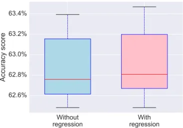
In the experiments, during time series extraction (step 2), we regress out all possible confounding factors, which includes movement estimation. In order to quantify the information contained in the movements, we try predict-ing ASD diagnosis with and without movement regression. FigureA1shows that no significant difference is observed with and without movement regression, which means that movement effect does not affect strongly our connectome estimation.
Movement-based prediction
Going further, we also perform the diagnosis directly based on movement estimations. Because movement pa-rameters are time-series, it is not possible to use them directly as features in a prediction task. For this pur-pose, we extract temporal descriptors from these series. These descriptors are similar to the ones extracted in FSL FIX [78], a tool to identify noisy ICA components: coeffi-cients of autoregressive models of several orders, kurtosis, skewness, entropy, difference between the mean and the median, and Fourier transform coefficients.
As for the prediction pipelines, we tried a wide range of strategies to predict from movement parameters. We ex-tracted the descriptors on the movements, the gradient of the movements, the gradient squared, and the framewise
Without
regression
regression
With
62.6%
62.8%
63.0%
63.2%
63.4%
Accuracy score
Figure A1: Prediction accuracy scores with and without per-forming movement regression during time series extraction. No significant difference is observed.
displacement. We tried several predictors (with and with-out feature extraction), logistic regression, SVC, Ridge classifier, Gaussian Naive Bayes and random forests.
We present the results obtained on the best predic-tion procedure. For each participant, 56 descriptors are extracted from the movement estimations and their gradi-ent, and are used as features in an SVC for diagnosis. We observe that the scores obtained using movements are at chance level. Note that we see a trend already observed on prediction based on connectomes: The variance of pre-diction scores is much larger for inter-site prepre-diction.
Right handed males Biggest All
9-18 yo sites subjects 3 sites Intra-site 53.2% 53.9% 53.5% 53.0% 54.3% Accuracy ±0.1% ±0.6% ±0.2% ±0.2% ±0.1% Inter-site 53.8% 54.3% 51.5% 52.8% Accuracy ±8.1% ±8.3% ±7.3% ±8.2%
Table A1: Prediction accuracy scores based on movements estimations. Results are similar across folds but variance of inter-site prediction is larger.
Figure A2: Comparison of prediction results obtained using 84 regions extracted from Harvard Oxford and Yeo atlases against the set of all regions extracted from them (labelled
as full ). Results obtained using 84 regions are better than full
atlases. This is probably due to the fact that small regions can
induce spurious correlations in the connectivity matrices.
Intra-site Inter-site
Figure A3: Classification accuracy scores using overlapping atlases and their non overlapping counterpart. Point above the identity line support the idea that fuzzy overlapping maps are better at predicting behavioral variable than non-overlapping.
45% 50% 55% 60% 65% SVC-2 Ridge classifier ANOVA + SVC-2 ANOVA + Ridge classifier SVC-1 Lasso
Without feature selection With feature selection
Figure A4: Comparison of prediction results obtained using feature selection or sparse methods. When selecting a reduced number of features, using either ANOVA to select 10% of the fea-tures, or sparsity inducing methods, we observe that the prediction accuracy drops compared to a classification using all features. This can be due to the fact that the connectivity matrices represent mixed features that should be handled together rather than seaprately. This may also be due to global effects in the connectivity: A global hypo-connectivity, as already observed in ASD patients, cannot be