HAL Id: tel-01358409
https://tel.archives-ouvertes.fr/tel-01358409
Submitted on 5 Sep 2016HAL is a multi-disciplinary open access archive for the deposit and dissemination of sci-entific research documents, whether they are pub-lished or not. The documents may come from teaching and research institutions in France or abroad, or from public or private research centers.
L’archive ouverte pluridisciplinaire HAL, est destinée au dépôt et à la diffusion de documents scientifiques de niveau recherche, publiés ou non, émanant des établissements d’enseignement et de recherche français ou étrangers, des laboratoires publics ou privés.
approach
Xuan-Nam Nguyen
To cite this version:
Xuan-Nam Nguyen. The OpenFlow rules placement problem : a black box approach. Other [cs.OH]. Université Nice Sophia Antipolis, 2016. English. �NNT : 2016NICE4012�. �tel-01358409�
ÉCOLE DOCTORALE STIC
SCIENCES ET TECHNOLOGIES DE L’INFORMATION ET DE LA COMMUNICATION
T H È S E
pour l’obtention du grade de
Docteur en Sciences
de l’Université de Nice - Sophia Antipolis
Mention : Informatique
Présentée et soutenue par
Xuan Nam NGUYEN
The OpenFlow Rules Placement Problem:
a Black Box approach
Thèse dirigée par Thierry TURLETTI et Walid DABBOUS Inria, France
Jury :
Rapporteurs : Giuseppe BIANCHI University of Rome Tor Vergata
Steve UHLIG Queen Mary University of London
Directeurs : Thierry TURLETTI Inria
Walid DABBOUS Inria
Examinateurs : Mathieu BOUET Thales
Laurent VANBEVER ETH Zurich
Président : Guillaume URVOY-KELLER University of Nice Sophia Antipolis
This thesis summarizes my research results during my Ph.D. study at the research team DIANA, Inria, France from 2012 to 2016.
Firstly, I would like to express my sincere gratitude to my advisor Dr. Thierry TURLETTI and Dr. Walid DABBOUS for their belief, patience, motivation, vision, and immense knowledge. Their guidance helped me to pass difficult moments of the research. It is my great pleasure to be their student.
Besides my advisors, I would like to thank Dr. Damien SAUCEZ, Dr. Chadi BARAKAT, and Dr. Truong Khoa PHAN for their brilliant ideas, discussions, valuable comments. They look like mentors, friends than professors, and I learned a lot from them.
I thank my DIANA fellow labmates, my co-authors, my collagues at Aalto University, and my friends for the time we were working together, for exchanges of knowledge, skills and for unfogettable moments we had in four years.
I recognize that this research would not have been possible without the financial support from Inria, the Nice Sophia Antipolis University, and I would like to express my gratitude to those agencies.
Last but not the least, I would like to thank my parents, my sisters, and my fiance Huong, for their sacrifice and unconditional support during these years. They have cherished with me every great moment and been beside me whenever I needed them.
Abstract: The massive number of connected devices combined with an ever increasing volume of data traffic push network operators to their limit by limiting their profitability. Software-Defined Networking (SDN), which decouples network control logics from forwarding devices, has been proposed to tackle this problem. An important part of the SDN concepts is implemented by the OpenFlow protocol that abstracts network communications as flows and processes them using a prioritized list of matching-actions rules on the network forwarding elements. While the abstraction offered by OpenFlow allows to implement a large panel of applications, it raises the new problem of how to define the rules and where to place them in the network while respecting all technical and administrative requirements, which we refer as the OpenFlow Rules Placement Problem (ORPP).
In this thesis, we focus on the ORPP, and propose a black box abstraction that can hide the complexity of rules management. First, we formalize that problem, classify, and discuss existing solutions. We discover that most of the solutions enforce the routing policy when placing rules, which is not memory efficient in some cases. Second, by trading routing for better resource efficiency, we propose OFFICER and aOFFICER, two complementary rules placement frameworks that select and place OpenFlow rules satisfying policies and network constraints, while minimizing overheads. The main idea of OFFICER and aOFFICER is to install rules on efficient paths for important, large flows, and let other flows follow default, less appropriate paths. On one hand, OFFICER is designed based on optimization techniques to solve the offline ORPP, in which the set of flows is assumed known and stable in a period. On the other hand, aOFFICER uses adaptive control techniques to cope with the online ORPP, where the set of flows is unknown and varies over time. These proposals are evaluated and compared extensively to existing solutions in realistic scenarios. Finally, we study a use case of the black box abstraction, in which we target to improve the performance of content delivery services in cellular networks.
Keywords: Software-Defined Networking, OpenFlow, Rules Placement,
1 Introduction 1
1.1 Problem Statement and Motivation . . . 1
1.2 Example Scenarios . . . 4 1.3 Research Methodology . . . 7 1.4 Thesis Outline . . . 7 1.5 Publications . . . 9 2 Preliminaries 11 2.1 Linear Programming . . . 11 2.2 Greedy Algorithms . . . 12
2.3 Exponentially Weighted Moving Average Model . . . 13
2.4 Increase/Decrease Algorithms . . . 14
3 Literature Review 17 3.1 Introduction. . . 17
3.2 OpenFlow Rules Placement Problem . . . 18
3.2.1 Problem Formalization. . . 18
3.2.2 Challenges . . . 20
3.3 Efficient Memory Management . . . 21
3.3.1 Eviction . . . 22
3.3.2 Compression . . . 24
3.3.3 Split and Distribution . . . 28
3.4 Reducing Signaling Overhead . . . 32
3.4.1 Reactive and Proactive Rules Placement . . . 33
3.4.2 Delegating Functions to OpenFlow switches . . . 34
3.5 Conclusion . . . 35
4 Offline Rules Placement in OpenFlow Networks 37 4.1 Introduction. . . 37
4.2 General Model to Allocate Rules in OpenFlow . . . 40
4.3 Rule Allocation Under Memory Constraints . . . 43
4.3.1 Minimizing Memory Usage . . . 44
4.3.2 Maximizing Traffic Satisfaction . . . 44
4.3.3 Heuristic . . . 45 4.4 Evaluation. . . 48 4.4.1 Methodology . . . 49 4.4.2 Results . . . 51 4.5 Discussion . . . 53 4.5.1 Routing Policy . . . 53 4.5.2 Rule Aggregation . . . 53
4.5.3 Multipath . . . 53
4.5.4 Related Work . . . 54
4.6 Conclusion . . . 55
5 Adaptive Rules Placement in OpenFlow Networks 57 5.1 Introduction. . . 57
5.2 aOFFICER: Adaptive OpenFlow Rules Placement . . . 59
5.2.1 Objectives. . . 59 5.2.2 Design . . . 60 5.2.3 Adaptive Threshold . . . 61 5.3 Evaluation. . . 66 5.3.1 Setup . . . 66 5.3.2 Adaptive Threshold . . . 69
5.3.3 Adaptive Timeout and Deflection Technique. . . 73
5.4 Conclusion . . . 77
6 Use Case: Improving Content Delivery in LTEs 79 6.1 Introduction. . . 79
6.2 Background . . . 81
6.3 LTE In-network Caching Architecture . . . 81
6.3.1 Multi-level Caching Scheme . . . 82
6.3.2 Enabling Backhaul Caching with OpenFlow . . . 83
6.4 Content Allocation Model . . . 83
6.4.1 Content Allocation Problem Approximation . . . 86
6.5 Evaluation. . . 87
6.5.1 Simulation Setup . . . 87
6.5.2 Benefits of Caching at Different Levels . . . 89
6.5.3 Impact of Several Levels Caching . . . 92
6.5.4 Advantages of Using Opportunistic Caching for Networks with Loss . . . 93
6.6 Related Work . . . 94
6.7 Conclusion . . . 95
7 Conclusions and Future Work 97 7.1 Conclusions . . . 97
7.2 Future Work . . . 99
7.2.1 Robust and Fault Tolerant Rules Placement . . . 99
7.2.2 Impact of Default Devices . . . 99
7.2.3 Multilevel Table Rules Placement. . . 99
7.2.4 Network Function Virtualization . . . 100
Acronym
CDF Cumulative Distribution Function PDF Probability Mass Function
IP Internet Protocol
ISP Internet Service Provider ILP Integer Linear Programming
MILP Mixed Integer Linear Programing MPLS Multi-protocol Label Switching OSPF Open Shortest Path First ECMP Equal Cost Multi-Path QoS Quality of Service
SDN Software-Defined Networking
TCAM Ternary Content Addressable Memory TE Traffic Engineering
WAN Wide Area Network
ORPP OpenFlow Rules Placement Problem LTE Long-Term Evolution
CCN Content-Centric Networking ICN Information-Centric Networking
ASIC Application-specific Integrated Circuit LRU Least Recently Used
Access control rule Rule having actions field drop/permit packets. Commodity switch OpenFlow switch that stores rules in TCAM. Default devices Devices (e.g., software OpenFlow switches) that store rules in non-TCAM (e.g., RAM), used to process non matching packets.
Default path Sequence of nodes from an ingress switch to the default devices, formed by default rules. Default rule Lowest priority rule, matching all the packets. Elephant flow Flow that sends many packets or bytes. Endpoint Policy Policy that defines the endpoints for each flow
(e.g., egress links, gateways, firewalls). Exact-matching rule Rule that does not contain ternary elements
(∗) in its matching pattern.
Flow table hit A flow is processed by a non-default rule. Flow table miss A flow is processed by the default rule. Flow table List of prioritized rules on the switch.
Flow A sequence of packets that have common
header fields (e.g., destination IP address). Forwarding rule Rule having the actions field forwarding
pack-ets to an interface.
Mouse flow Flow that sends few packets or bytes.
Routing policy Policy that specifies the path that the flow must follow.
Rule space Set of all possible rules for selection.
Rules placement A configuration that indicates which rules are placed on which switch.
Rule An instruction for the OpenFlow switch speci-fying how to process the packets.
Wildcard rule Rule that contains ternary elements (∗) in its matching pattern.
Introduction
Contents
1.1 Problem Statement and Motivation . . . . 1
1.2 Example Scenarios. . . . 4
1.3 Research Methodology . . . . 7
1.4 Thesis Outline . . . . 7
1.5 Publications. . . . 9
1.1
Problem Statement and Motivation
Nowadays, the Internet is an integral part of our modern life, and it has revolutionized the way we communicate. Due to technology advances, more people can access to the Internet using cheaper, more portable, more powerful devices (e.g., mobile phones, tablets, laptops). In recent years, the number of Internet-connected devices and the traffic volume have increased dramatically. Facebook, the most popular social network, has reached one billion users in a single day [Fac]. According to a Cisco’s report [Cis15], the number of Internet connected devices was nearly two per capita in 2014, and will be three per capita in 2019. Furthermore, the annual global traffic has increased five times in the past five years (2009-2014), will surpass the zettabyte (1021 bytes) in 2016 and two zettabytes in 2019. Also, the video streaming traffic (e.g., Video-on-Demand, IPTV) accounts for 64% of all Internet traffic in 2014, and that portion will be 80% in 2019.
To keep pace with increasing demands, Internet Services Providers (ISP) often have to upgrade and reconfigure the network, e.g., buying and configuring new net-work devices. Normally, operators often have to transform high-level policies (e.g., the firewall policy, the routing policy) into low-level, vendor-specific configuration commands for each device, while manually adapting them to cope with network changes. However, this process is complicated, error-prone and time-consuming because of a large number of diverse network devices, such as switches, routers, mid-dleboxes. Automatic reconfiguration does not exist in current networks [KREV+15]. The primary reason for this inconvenience is the vertical integrated, tightly coupled architecture of network devices and the proprietary software controlling them. With this architecture, the network devices are closed boxes, which are hard for operators to innovate. If operators want a new feature, they often have to wait until next
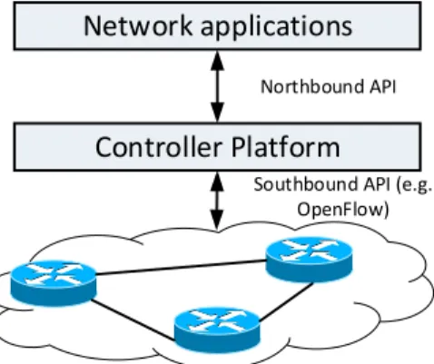
Controller Platform Network applications
Southbound API (e.g. OpenFlow) Northbound API
Data forwarding elements (e.g. OpenFlow switches)
Figure 1.1: SDN architecture
device life cycles or firmware releases from vendors. This inconvenience may slow down the operators’ development plans and incur high management costs.
To accelerate the innovation process, the operators need more flexibility to control, to customize network devices. To that goal, Software-Defined Networking (SDN) [NMN+14, XWF+15, KREV+15] advocates the separation between
forward-ing devices (the data plane) and the network control logic (the control plane). There exists similar ideas that did not succeed in the past, for example, in Active Net-working [TSS+97]. However, by appearing at the intersection of ideas, technology maturity and future needs, SDN offers a new potential approach to many existing and new network problems [NMN+14].
Fig. 1.1shows the SDN architecture. The separation of the control plane and the data plane is realized by a well-defined southbound application programming interface (API). In SDN, network control logic is implemented in an entity, called the controller. The controller is logically centralized but can be physically distributed for scalability. Also, a switch may have multiple controllers for fault tolerance and robustness. Via the southbound API, the controller directly manages the state of forwarding devices to respond to a wide range of network events, for example, when a link is congested, the controller reroutes active flows using this link to other paths. Furthermore, the controller exposes high level northbound APIs for operators to implement high level policies (e.g. firewall, load balancing). With this architecture, SDN promises to reduce costs and to simplify network management thanks to commodity, open forwarding hardwares, and high level management interfaces.
OpenFlow [MAB+08a] is the most popular implementation of the SDN south-bound API [NMN+14, XWF+15, KREV+15, JKM+13, KSP+14]. Although Open-Flow starts as academic experiments, it is receiving much attention from both academic and industry. Many vendors have supported OpenFlow in their commer-cial products [NMN+14]. As an example, Google is using OpenFlow in its WAN for traffic engineering applications [JKM+13]. Open Network Foundation [Fou13], an
Forward to port A Modify header fields Drop
IP src/dst , port number, VLAN
MATCHING ACTIONS COUNTERS
OPENFLOW SWITCH
Packets, Bytes, Duration Flow Table 1 Flow Table N
CONTROLLER APPLICATION Northbound API OpenFlow Protocol Traffic Firewall Learning Switch Load Balancing Topology Manager Device Manager Statistics
Figure 1.2: OpenFlow Architecture [NMN+14]
industrial-driven organization including the biggest operators (e.g., Google, Face-book, Yahoo, Microsoft) is improving the OpenFlow specification [Ope15b], and promoting OpenFlow as the standard southbound API of SDN.
The architecture of OpenFlow is depicted in Fig. 1.2. Forwarding devices are called OpenFlow switches, and all forwarding decisions are flow-based instead of destination-based like in traditional routers. An OpenFlow switch consists of flow tables, each containing a prioritized list of rules that determine how packets are processed by the switch.1 A rule consists of three main components: a matching pattern, an actions field and a counter. Generally, a matching pattern is a sequence of 0 − 1 bits and “don’t care" (denoted as ∗) bits, that forms a predicate for packet meta-information (e.g., src_ip = 10.0.0.∗). All packets making true the matching pattern predicate are said to belong to the same flow.
The actions field specifies the actions applying to every packet of the correspond-ing flow, e.g., forwardcorrespond-ing, droppcorrespond-ing, or rewritcorrespond-ing the packets. Finally, the counter records the number of processed packets (i.e., that made the predicate hold true) along with the lifetime of this rule. As a packet may match multiple matching patterns of different rules, each rule is associated with a priority number. Only the rule with the highest priority number that matches the packet is considered to take actions on it. The prioritization of rules permits constructing default actions that can be applied on packets only if no other rule can be used. Examples of default actions are dropping packets, or forwarding to a default interface. For efficiency and flexibility reasons, the latest versions of OpenFlow [Ope15b] support pipeline processing where a packet might be processed by several rules from different flow tables.
The behavior of an OpenFlow switch strongly depends on the set of rules it holds. With appropriate rules, an OpenFlow switch can act like a Layer-2 switch, a router, or a middlebox. Also, many network applications can be implemented using
1We follow the OpenFlow model terminology where a packet consists of any piece of information
OpenFlow, e.g., monitoring, accounting, traffic shaping, routing, access control, and load balancing [MAB+08a]. To implement these applications and operators policies, it is important to select and install corresponding rules on each OpenFlow switch. However, most of popular controller platforms [GKP+08, Flo15, Eri13] still force operators to manage their network at the level of individual switches, by selecting and installing rules to satisfy network constraints and policies [KLRW13]. Installing inappropriate rules may lead to frequently usages of default actions (e.g., forwarding to the controller), that may overload the controller and degrade network performance, such as packet latency.
Beyond flow abstraction provided by OpenFlow, our motivation is to raise the network abstraction towards a higher one: the black box. Using the black box abstraction, operators do not need to care about the complexity and diversity of underlying networks, and how to manage resources efficiently. Furthermore, operators can focus on specifying high level policies, which will be automatically compiled into appropriate OpenFlow rules.
To realize the blackbox abstraction, it is important to study and propose solu-tions for the problem of selecting and distributing OpenFlow rules, referred as the OpenFlow Rules Placement Problem (ORPP). This problem is not trivial, because in production networks, many rules are required and available for selection [MYSG12], but only a limited amount of resources, and in particular memory [SCF+12], is available on OpenFlow switches. Also, the ORPP is NP-hard in general, as we show in Chapter 4. Despite its complexity, solving this problem is essential to realize the black box abstraction.
1.2
Example Scenarios
In the following, we describe two representative scenarios, that motivate why Open-Flow is needed and why ORPP is challenging.
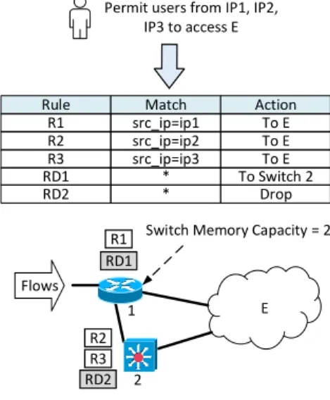
Access Control As a part of endpoint policy, the firewall policy is critical to the network security. Most of firewall policies can be defined as a list of prioritized access control rules, that specify which flows are authorized and where. OpenFlow is a potential candidate to implement access control applications, because it supports flexible matching patterns and multiple actions.
Ideally, all access control rules should be placed on the ingress switches to filter unwanted network traffic. However, the switch memory constraints prohibit placing all rules in ingress switches. An alternative solution is to put all rules in the software switches having large memory capacity (e.g. RAM), and to direct all traffic to them. However, software switches are generally slower than hardware-accelerated switches (e.g. using TCAM), because of high lookup delay. Therefore, a solution is required to select and distribute rules over all the switches such that the semantic of the original access control list is preserved, and resource constraints are satisfied.
R3 R1 R2 F1 F2 E1 2 1 3 Block traffic to 10.0.0.1 or to port 22 or from 10.0.0.2
Switch Memory Capacity = 3 R1
RD1
RD1 RD2
Rule Match Action
R1 R2 R3 RD1 dst_ip=10.0.0.1 Drop dst_port=22 Drop src_ip=10.0.0.2 Drop * To Switch 2 RD2 * E1
Figure 1.3: An example of access control rules placement. The firewall policy is compiled into a list of rules R1, R2, R3 for blocking matching packets, and two default rules RD1, RD2 for forwarding non-matching packets towards the endpoint E. These rules are distributed on several switches to ensure that flows F 1 and F 2 pass through all rules R1, R2, R3 to enforce the firewall policy.
R3 R4 R1 R2 F1 F2 E2 E1 2 1 3 F1 exits at E1 F2 exits at E2
Rule Match Action
R1 R2 R3 R4 F1 To Switch 2 F2 To Switch 3 F1 To E1 F2 To E2
Figure 1.4: An example of forwarding rules placement. Forwarding rules are installed on appropriate paths to make sure that the endpoint policy is satisfied. Rules R1, R3 (resp. R2, R4) are installed on switches 1, 2 (resp. 1, 3) to route F1 (resp. F2)
towards its endpoint E1 (E2).
must be enforced on all flows originated from switch 1 and 3. A solution is to use rules R1, R2, R3 for blocking matching packets, and use the default rules RD1, RD2 for forwarding non-matching packets towards endpoint E. Then, these rules are distributed on the switches, according to the memory capacity, to enforce the firewall policy on all flows.
Traffic engineering The role of the network is to deliver packets towards their destinations and to satisfy the operator’s requirements (e.g., low latency, low loss rate). OpenFlow allows defining rules matching any type of packets and forwarding them on any paths, which promises to support a wide range of policies.
Normally, the forwarding rules matching the packets should be placed on the shortest paths from their sources to their endpoints, to satisfy traffic engineering goals (e.g., delay, throughput). However, due to switch memory limitations, all required rules may not be fit into the shortest paths. Therefore, it is important to select and install forwarding rules on the appropriate paths, to satisfy requirements.
An example of forwarding rules placement is shown in Fig. 1.4. Both flows F 1, F 2 must be forwarded to their corresponding endpoint E1, E2. To that aim, a solution is to install forwarding rules R1, R3 (resp. R2, R4) on switches 1, 2 (resp. 1, 3) to route F 1 (resp. F 2) towards its endpoint E1 (resp. E2).
1.3
Research Methodology
Our motivation is to realize the black box abstraction using OpenFlow. To that aim, it is important to understand the ORPP, what are its challenges and existing ap-proaches. Even there are some OpenFlow surveys [XWF+15, KREV+15,NMN+14], but none of them formalizes and discusses that problem comprehensively. There-fore, we first propose a formalization for the problem, classify and discuss existing solutions to find new insights and new potential approaches.
After finding a new potential approach, we use it to address two instances of the problem: (i) the offline ORPP, in which the set of traffic flows is known and stable in a period, and (ii) the online ORPP, in which the set of flows is unknown and varies over time. Each assumption allows to apply well-known techniques to solve them. More precisely, we apply optimization techniques for the first instance, and adaptive control techniques for the second one.
For both instances, our goal is to design algorithms that generate rules satisfying policies, network constraints (e.g., memory, bandwidth) while reducing the costs, in terms of the signaling load and default load.2 On one hand, reducing the signaling load allows the controller to handle more devices and to process requests faster. On the other hand, reducing the default load also improves the network performance. For example, software switches’s processing introduces a higher delay than ASIC processing. By reducing the load on these devices (i.e., the default load), the total network delay can be improved.
To evaluate and to compare our proposals to existing solutions, we implement numerical and packet-level simulators using Python. Python is used because of its simplicity, and that it supports network simulation libraries (e.g., NetworkX [Net15], FNSS [SCP13]). Our experiments are performed on cluster platforms such as INRIA NEF [INR15], that allow performing simulations with many configurations simultaneously. Both real and synthetic inputs (e.g., topologies and packet traces) are considered. The outputs are analyzed using Pandas [Pan] and visualized using Matplotlib [Mat]. Beside simulations, some of our proposals (e.g., Wrapper [NST13b,
NST13a]) are verified on emulators (e.g., Mininet [LHM10]) and on a commodity
OpenFlow switch (Pronto 3290 [PRO15]).
1.4
Thesis Outline
In the following, we summarize the content of each chapter and the obtained results. In Chapter2, we present the basic preliminaries used in this thesis. This chapter includes Linear Programming to model optimization problems, Greedy heuristics to find approximate solutions, Exponentially Weighted Moving Average (EWMA) to model and predict future means of a variable, and Increase/Decrease algorithms to adapt a parameter.
2load on the default devices (e.g., software OpenFlow switches) that are used to process
In Chapter 3, we present background related to the fundamental problem of how to select rules and their locations such that network constraints and policies are respected, referred as the OpenFlow Rules Placement Problem (ORPP). First, we formalize that problem, and identify two main challenges, including resource limitations and the signaling overhead. Second, we classify, and discuss pros and cons of existing solutions extensively. In the best of our knowledge, this is the first survey focusing on the ORPP.
In Chapter4, we analyze and demonstrate a limitation of existing solutions. To satisfy endpoint policy, most of existing solutions [KHK13, KLRW13] place rules to enforce flows following the shortest paths. This constraint is sometimes necessary to meet the traffic engineering goals (e.g., low latency). However, in some cases, strictly enforcing this constraint may lead to unfeasible rules placement due to resource constraints (e.g., switch memory). Also, we believe that with the blackbox abstraction, operators do not need to care about the path selection, and can delegate the decision for the controller. Therefore, we propose to trade routing for better resource efficiency, to increase the number of possible paths for rules placement. This approach comes the fact that flows may follow a longer path, but it is compensated by better resource utilization.
Using the new approach, we study the offline ORPP, in which the set of flows is known and stable in the considered period. First, we propose a heuristic that selects the paths consuming less memory, called the deflection technique. Second, we prove that the offline ORPP is NP-Hard and formalize it as an Integer Linear Programming (ILP). That model supports various objective functions, and includes necessary constraints such as memory, endpoint policies, bandwidth constraints. Optimal rules can be found by solving that ILP using LP solvers, such as CPLEX [IBM]. A Greedy heuristic, called OFFICER, is designed to find rules in polynomial time complexity for the problem instance with large inputs, e.g., large number of flows. We then perform numerical simulations in realistic scenarios, to compare OFFICER to the optimum and a random rules placement solution.
In reality, flows are often unknown and hard to predict accurately [BAAZ11]. Therefore, the solutions proposed in Chapter4 can not be directly applied when flows are unknown. In Chapter 5, we study the online ORPP, in which the set of flows is unknown and varies over time. To solve this problem, existing controller platforms [Flo15,GKP+08,Eri13] treat all flows equally and place rules reactively. However, this approach has several cons. First, it incurs a high signaling load, a high latency due to many flows. Second, rules for large flows may not be installed because resources are already occupied by other flows. As consequences, policies can be violated, and network performance are degraded.
We argue that in case of resource limitations (e.g., switch memory), only rules for important, large flows should be installed. To that goal, we propose aOFFICER, an adaptive rules placement framework, that can detect candidate flows and install rules for them on efficient paths. Furthermore, aOFFICER can adapt the parameter automatically to respond to fluctuations in flow demands. Our simulation results in realistic scenarios confirm that aOFFICER can reduce costs and does not introduce
large signaling overhead, compared to existing solutions.
With the black box abstraction, operators can implement high level, flexible endpoint policies using OpenFlow, thanks to algorithms OFFICER and aOFFICER proposed in Chapter 4and 5. In Chapter6, we exploit a use case of the black box abstraction, in which we improve the performance of content delivery services in cellular networks.
Nowadays, traffic from content delivery services will continue to grow in coming years, which increases CAPEX and OPEX of network management significantly. OpenFlow is a potential approach to address this problem. First, OpenFlow can enable in-network caching functionalities (e.g., using our technical solution [NST13b,
NST13a]), so caches can be deployed everywhere in the network. Second, we propose
a novel caching framework, named Arothron. The main idea is to split the cache storage on each node into two parts: one uses opportunistic caching, and the other uses preset caching. On one hand, opportunistic caches, which store and replace contents using the LRU mechanism, can absorb short term fluctuations in content demands. On the other hand, preset caches, which store popular contents, can satisfy long term content demands with high cache hit ratios. To decide which content is stored in which preset cache, a Mixed Linear Integer Programming and a Greedy heuristic are used. With extensive simulations in realistic scenarios, we show that network performances are better if each storage unit combines both opportunistic and preset caching, compared to using only opportunistic caching or using only preset caching. Second, we observe that the optimal ratio between the opportunistic and the preset cache on each node is not the same, and it depends on the node location.
Finally, in Chapter 7, we summarize the content of the thesis, and discuss potential research directions.
1.5
Publications
The complete list of my publications is the following. International Journals
[WNTS16] M. Wetterwald, X.N. Nguyen, T. Turletti, and D. Saucez, “SDN
for Public Safety Networks”, under submission, 2016
[NSBT15b] X.N. Nguyen, D. Saucez, C. Barakat and T. Turletti, “Rules
Placement Problem in OpenFlow Networks: a Survey”, IEEE Communica-tions Surveys and Tutorials, October 2015 (Impact Factor: 6.490)
[NMN+14] BAA Nunes, M. Mendonca, X.N. Nguyen, K. Obraczka, T. Turletti, “A Survey of Software-Defined Networking: Past, Present, and Future of Programmable Networks”, IEEE Communications Surveys and Tutorials, February 2014 (Impact Factor: 6.490)
International Conferences, Workshops
[KNS+15] M. Kimmerlin, X.N. Nguyen, D. Saucez, J. Costa-Requena and T. Turletti, “Arothron: a Versatile Caching Framework for LTE”, under
submission, 2015
[NSBT15a] X.N. Nguyen, D. Saucez, C. Barakat and T. Turletti, “OFFICER:
A general Optimization Framework for OpenFlow Rule Allocation and Endpoint Policy Enforcement”, IEEE INFOCOM 2015, Hongkong, China, April 2015 (acceptance ratio: 19%)
[NSBT14] X.N. Nguyen, D. Saucez, C. Barakat and T. Turletti, “Optimizing
rules placement in OpenFlow networks: trading routing for better effi-ciency”, ACM HotSDN 2014, Chicago, United States, August 2014 (acceptance ratio: 28.9%)
[NST13a] X.N. Nguyen, D. Saucez and T. Turletti, “Efficient caching in
Content-Centric Networks using OpenFlow”, IEEE INFOCOM 2013 Work-shop Proceedings, Turin, Italy, April 2013 (acceptance ratio: 14.3%)
Research Reports
[NST13b] X.N. Nguyen, D. Saucez and T. Turletti, “Providing CCN
func-tionalities over OpenFlow switches”, INRIA Research Report 00920554, 2013
[Ngu12] X.N. Nguyen, “Software Defined Networking in Wireless Mesh
Preliminaries
Contents
2.1 Linear Programming . . . . 11
2.2 Greedy Algorithms . . . . 12
2.3 Exponentially Weighted Moving Average Model . . . . 13
2.4 Increase/Decrease Algorithms. . . . 14
In this chapter, we present some preliminaries that we use throughout this thesis.
2.1
Linear Programming
Linear Programming (LP) is a general method to model and to achieve the best outcomes of many combinatorial problems [Sch86,Chv83], such as the 0-1 Knapsack problem. Given a set of items with different weights and values, the motivation of the 0-1 Knapsack problem is to find which item should be selected, such that the total weight is less than or equal to a given limit, and the total value is as large as possible.
LP is widely applied to various domains, such as business, economic, engineering. LP has proved its useful in modeling and solving diverse types of problems (e.g., planning, scheduling, assignment).
Basically, a LP is composed of a linear objective function, a set of linear inequality constraints formalized by variables (i.e., the problem outputs) and parameters (i.e., the problem inputs). The objective function represents the optimization target, and it can be written in terms of minimizing or maximizing, e.g., minimizing memory consumption, maximizing user satisfaction. If the goal is just to find feasible solutions satisfying constraints, the objective function can be omitted. Normally, a LP is expressed as:
max{cTx : Ax ≤ b; x ≥ 0} (2.1)
In Eq. 2.1, x represents the vector of variables, b, c are vectors of coefficients, A is matrix of coefficients, and (.)T is the matrix transpose function.
If some variables in x are integrals, the LP is called a Mixed Integer Linear Programming (MILP). if all variables in x are integrals, the LP is called an Integer
Linear Programming (ILP). For example, the 0-1 Knapsack problem mentioned above can be represented as the following ILP:
max{ n X i=1 vixi : n X i=1 wixi≤ W ; xi ∈ {0; 1}} (2.2)
In Eq. 2.2, W is the weight limit; vi, wi are the value and the weight of item i; x is
the binary variable that indicates if item i is selected (xi= 1) or not (xi = 0).
The problem in the form 2.1 is called the primal problem, and there exists a dual problem:
min{bTy : ATy ≥ c; y ≥ 0} (2.3)
The objective of dual problem, at any feasible solution, is always greater than the primal’s objective function, at any feasible solution. Furthermore, if the primal problem has an optimal solution x∗, then its dual has an optimal solution y∗, such that:
cTx∗ = bTy∗ (2.4)
These above properties are often used to find bounds for the objective function. In some cases, bounds are also used as a stopping condition for solving algorithms. Due to its wide applications, many methods have been proposed to solve LP, such as cutting plane, brand and bound, column generation, and row genera-tion [Sch86,Chv83]. These methods are usually implemented in LP solvers (e.g., CPLEX [IBM], GLPK [GNU13]), which can find exact and approximate solutions for the problem. A brief view of popular solvers can be found in [CCK+10]. In our study, we use CPLEX [IBM] because it outperforms other open-source solvers in many cases [MT13], and it is free for academic use.
In this thesis, we apply LP to model OpenFlow Rules Placement Problem as an ILP (Chapter 4) and the content placement problem as a MILP (Chapter 6). These LPs are then implemented on CPLEX to find the optimal placements for rules and contents.
2.2
Greedy Algorithms
In general, most of placement problems are NP-Hard, which means that there is no known polynomial-complexity algorithms to find the optimal solutions. Therefore, using LP solvers for large problem instances (e.g., large number of variables, large number of constraints) is not practical due to a large execution time.
To cope with this limitation, heuristics are used to find near optimal solutions in acceptable execution time. Starting from a trivial solution, a heuristic tries to improve the solution in each step, and terminates when the obtained solution is good enough. There are many popular heuristics, such as Greedy, Simulated Anneal [Sch86]. Each heuristic and their parameters are implemented and optimized differently for different problems.
To evaluate the performance of a heuristic, the approximation factor (or approx-imation ratio) p is used. A heuristic is called p-approxapprox-imation if for any inputs, heuristic’s objective value over optimum objective value is at least p.
Greedy is a common heuristic, widely used in different domains, for example, machine learning, artificial intelligence. In ad-hoc mobile networks, Greedy is also used to route packets with the fewest number of hops and the smallest delay.
Basically, Greedy follows the locally optimal choice in each step with the hope of finding the global optimum. For example, to find solutions for the 0-1 Knapsack problem, one possible greedy strategy is that in each step, the unselected item with maximum value of (vi/wi) is selected. In many problems, Greedy does not
guarantee to find the global optimum, but it can approximate the global optimum in a reasonable execution time. For example, Greedy has been proven that it is 1/2-approximation for the Knapsack problem [Sch86].
Using Greedy, the solution for small problem instances can be easy and straight-forward. However, for large problem instances, in some cases, short term decisions may lead to worst long term outcome.
Basically, a Greedy has the following components: • A candidate set, from which a solution is created.
• A selection function, which decides how to select the best candidate for a set. • A feasible function, which checks if a candidate can be selected.
• A stop condition, which indicates when the algorithm should stop.
For example, in Knapsack problem, the candidate set is the set of items. The selection function picks the largest-value item among available items. After that, this item is checked by the feasible function (e.g., if its weight < the available capacity). If the item can be added, it is marked as selected. Then, the same process is repeated for the rest of items. Finally, Greedy returns the solutions when all items are verified or the stop condition is satisfied (e.g., if the available capacity < 5% total capacity).
In this thesis, we design our heuristics based on Greedy, to find rules placement solutions in Chapter4 and content placement solutions in Chapter6. The key ideas of these heuristics are to install rules for the largest flows, or to place the most popular contents first, since they contribute most to the objective function. The evaluation results in realistic scenarios confirm the simplicity and the efficiency of these heuristics, compared to the optimum.
2.3
Exponentially Weighted Moving Average Model
In statistics, a moving average is the average that moves. More precisely, it is a set of numbers, each corresponding to the average of a subset of a larger data set. A moving average is commonly used to analyze financial data, such as stock prices,
to get an overall idea about the trend of the data set. Furthermore, it can smooth out short-term fluctuations, and forecast long term trends. Mathematically, it can also be considered as a low pass filter, where high frequencies (e.g., short term fluctuations) are removed from the original signal.
For example, given a time series D = {1, 3, 2, 3, 4, 5} that represents the price of a stock in each day. 3-days moving average Si, represents the evolving of the stock
prices, is computed based as the average price of 3 consecutive days:
S1 = (1 + 3 + 2)/3 = 2 (2.5)
S2 = (3 + 2 + 3)/3 = 2.33 (2.6)
S3 = (2 + 3 + 4)/3 = 3 (2.7)
S4 = (3 + 4 + 5)/3 = 4 (2.8)
There are different kinds of moving averages. An Exponential Weighted Moving Average (EWMA) model [KO90] is a kind of moving average, where the weight factor of each older datum decreases exponentially with ages. EWMA has an advantage compared to simple MA, as EWMA remembers a fraction of its history and accounts them in future values. Given a time series X = {X0, X1, ...}, the EWMA for a time series X is calculated recursively as the following:
S0 = X0 (2.9)
St+1= αSt+ (1 − α)Xt (2.10)
In Eq. 2.10, Xt, St are the variable value, and the EWMA at time t. The
parameter 0 < α ≤ 1 represents the weight contributed of old samples into the future mean value. Smaller α discounts old samples faster, and highlights the important of the most recent sample. Higher α indicates slow decay in time series, in other terms, the time series falls off more slowly. Selecting the right value of α is a matter of preferences and experiences.
In Chapter5, we apply the EWMA model to estimate the future mean value for a time series of binary installation trials (0: fail, 1: success).
2.4
Increase/Decrease Algorithms
The Increase/Decrease (ID) algorithm is a type of feedback control algorithms, best known for its use in TCP Congestion Avoidance [APB09], to adjust the transmission rate (window size) of the transmitters.
ID algorithms combines addictive/multiplicative (denoted as A/M) increasing and addictive/multiplicative decreasing to adjust a parameter, when conditions are satisfied or periodically. For example, in TCP Congestion Avoidance, AIMD algorithm is used. More precisely, the transmission rate is addictive increasing (AI) by a fixed amount for every round trip time. When the congestion (e.g., loss occurs) is detected, the transmitter decreases the transmission rate by a multiplicative factor (1/2). Moreover, if multiple flows use AIMD algorithms, they will eventually
converge to use an equal amount of link capacity. Other types of ID algorithms, such as MIMD and AIAD, do not converge for this case.
Basically, an ID algorithm can be expressed as follows:
Wt+1= M1∗ Wt+ A1 (2.11)
Wt+1= Wt/M2− A2 (2.12)
In Eq. 2.11and2.12, Wt is the value of the variable at time t, M1, A1, M2, A2 ∈ [0; ∞) are constant addictive/multiplicative factors. There values are selected based on experiences, and they affect to the convergence speed, size of oscillations, and the possible values of the control parameter. Depending on conditions, increasing phase (Eq. 2.11) or decreasing phase (Eq. 2.12) is called.
In Chapter 5, we use the MIMD algorithm to adjust the threshold H according to the average success rate r (estimated using EWMA model) periodically. More precisely, H is multiplicative increasing when the r < r0 (r0 is an expected value for r), and multiplicative decreasing when r > r0. The MIMD algorithm is used because it quickly converges in our scenarios.
Literature Review
Contents
3.1 Introduction . . . . 17
3.2 OpenFlow Rules Placement Problem. . . . 18
3.2.1 Problem Formalization. . . 18 3.2.2 Challenges . . . 20 3.3 Efficient Memory Management . . . . 21
3.3.1 Eviction . . . 22 3.3.2 Compression . . . 24 3.3.3 Split and Distribution . . . 28 3.4 Reducing Signaling Overhead . . . . 32
3.4.1 Reactive and Proactive Rules Placement . . . 33 3.4.2 Delegating Functions to OpenFlow switches . . . 34 3.5 Conclusion . . . . 35
In this chapter, we review the state of the art around the problem of selecting and distributing OpenFlow rules, which we refer as OpenFlow Rules Placement Problem. To the best of our knowledge, this is the most comprehensive survey about the OpenFlow Rules Placement Problem, including a formalization, a classification, and a discussion of the related work. The remainder of this chapter corresponds to our publication [NSBT15b].
3.1
Introduction
Computer networks today consist of many heterogeneous devices (e.g., switches, routers, middleboxes) from different vendors, with a variety of sophisticated and distributed protocols running on them. Network operators are responsible for configuring policies to respond to a wide range of network events and applications. Normally, operators have to manually transform these high level policies into low level vendor specific instructions, while adjusting them according to changes in network state. As a result, network management and performance tuning are often complicated, error-prone and time-consuming. The main reason is the tight coupling of network devices with the proprietary software controlling them, thus making it difficult for operators to innovate and specify high-level policies [MAB+08a].
Software-Defined Networking (SDN) advocates the separation between forwarding devices and the software controlling them in order to break the dependency on a particular equipment constructor and to simplify network management. In particular, OpenFlow implements a part of the SDN concept through a simple but powerful protocol that abstracts network communications in the form of flows to be processed by intermediate network equipments with a minimum set of primitives [MAB+08a].
OpenFlow offers many new perspectives to network operators and opens a plethora of research questions such as how to design network programming languages, obtain robust systems with centralized management, control traffic at the packet level, perform network virtualization, or even co-exist with traditional network protocols [FHF+11, VKF12, VWY+13, NMN+14, XWF+15, KREV+15, VCB+15]. For all these questions, finding how to allocate rules such that high-level policies are satisfied while respecting all the constraints imposed by the network is essential. The challenge being that while potentially many rules are required for traffic management purpose [MYSG12], in practice, only a limited amount of resources, and in particular memory [SCF+12], is available on OpenFlow switches. In this chapter, we survey the fundamental problem when OpenFlow is used in production networks, that we refer to it as the OpenFlow Rules Placement Problem. We focus on OpenFlow as it is the most popular southbound SDN interface that has been deployed in production networks [JKM+13].
The contributions of this chapter include:
• A generalization of the OpenFlow rules placement problem and an identification of its main challenges involved.
• A presentation, classification, and comparison of existing solutions proposed to address the OpenFlow rules placement problem.
This chapter is organized as follows. In Sec. 3.2, we formalize the OpenFlow rules placement problem, discuss the challenges. We continue with existing ideas that address the two main challenges of the OpenFlow rules placement problem: memory limitation in Sec. 3.3, and signaling overhead in Sec.3.4.
3.2
OpenFlow Rules Placement Problem
3.2.1 Problem Formalization
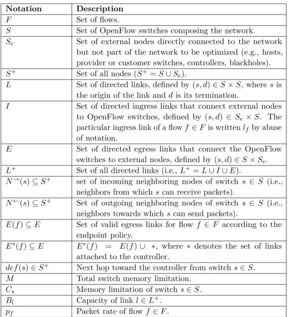
In the following, we formalize the OpenFlow Rules Placement Problem using the notations in Table3.1.
The network is modeled as a directed graph G = (V, E), where V is the set of nodes and each node v ∈ V can store Cv rules, E is the set of directed links of the
network. O is the set of endpoints where the flow used to exit the network (e.g., peering links, gateways, firewalls). A flow can have many endpoints of ∈ O. P is
the set of possible paths that flows can use to reach their endpoints of ∈ O. Each path p ∈ P , consists of a sequence of nodes v ∈ V . F , R are the set of flows and rules for selection, respectively.
Table 3.1: Notations used in this chapter Notation Definition
V set of OpenFlow nodes
E set of links
O set of endpoints (e.g., peering links)
F set of flows (e.g., source – destination IP flows) R set of possible rules for selection
T set of time values
F T (v, t) flow tables of node i at time t ∈ T
Cv memory capacity of node v (e.g., in total number of rules)
P set of possible paths to the endpoints (e.g., shortest paths) m matching pattern field (e.g., srcIP = 10.0.0.∗)
a actions field (e.g., dropping the packets) q priority number (0 to 65535)
tidle idle timeout (s)
thard hard timeout (s)
EP endpoint policy, defines the endpoint(s) o ∈ O of f ∈ F RP routing policy, defines the path(s) p ∈ P of f ∈ F
The output of the problem is the content of the flow table of node F T (v, t) = [r1, r2, ...] ⊂ R, which defines the set of rules required to install node v ∈ V at time t ∈ T . T = [t1, t2, ...] is the set of the time instants at which F T (v, t) is computed and remains unchanged during the period [ti, ti+1]. Each rule rj is defined as a
tuple, which contains values for matching pattern m, actions a, priority number q and timeouts tidle, thard, selected by the solvers.1 The flow table content of all nodes
F T (v, t), ∀v ∈ V at a time t is defined as a rules placement solution. Furthermore, F T (v, t) changes over time t to adapt with network changes (e.g., topology changes, traffic fluctuation). In order to construct rules placement, the following inputs are considered:
• Traffic flows F , which stand for the network traffic. The definition of a flow, implemented with the matching pattern, depends on the granularity needed to implement the operator policies. For example, network traffic can be modeled as the set of Source-Destination (SD) flows, each flow is a sequence of packets having the same source and destination IP address.
• Policies, which are defined by the operator, can be classified into two cate-gories: (i) the end-point policy EP : F → O that defines where to ultimately deliver packets (e.g. the cheapest link) and (ii) the routing policy RP : F → P that indicates the paths that flows must follow before being delivered (e.g., the shortest path) [KLRW13]. The definition of these policies is often the result
1We focus on important fields only. The complete list of fields of an OpenFlow rule can be found
of the combination of objectives such as cost reduction, QoS requirements and energy efficiency [GMP14,NSBT15a,HLGY14,KLRW13,LLG14].
• Rule space R, which defines the set of all possible rules for selection, depend-ing on applications. For example, an access control application allows selectdepend-ing rules that contain matching m for 5-tuples IP fields (source/destination IP address, source/destination port number, protocol number) while a load balanc-ing application requires rules that contain matchbalanc-ing m for source/destination IP address [WBR11]. The combination of fields and values forms a large space for selection.
• Resource constraints, such as memory, bandwidth, CPU capacity of the controller and nodes. Rules placement solutions must satisfy these resource constraints. As an example, the total number of rules on a node should not exceed the memory capacity of the nodes: |F T (v, t)| ≤ Cv, ∀(v, t) ∈ V × T .
There might be a countless number of rules placement possibilities that sat-isfy the above inputs. Therefore, F T (v, t) is usually selected based on additional requirements, such as in order to minimize the overall rule space consumption
P
v∈V |F T (v, t)|. Note that in general, the OpenFlow Rules Placement problem is
NP-hard, as we will proof in Chapter 4by reducing it to the Knapsack problem.
3.2.2 Challenges
Elaborating an efficient rules placement is challenging due to the following reasons.
3.2.2.1 Resource limitations
In most of production environments, a large number of rules is required to support policies whereas network resources (e.g., memory) are unfortunately limited. For ex-ample, up to 8 millions of rules are required in typical enterprise networks [YRFW10] and up to one billion for the task management in the cloud [MYSG12]. According to Curtis et al. [CMT+11], a Top-of-Rack switch in data centers may need 78,000 rules to accommodate the traffic.
While the number of rules needed can be very large, the memory capacity to store rules is rather small. Typically, OpenFlow flow tables are implemented using Ternary Content Addressable Memory (TCAM) on switches to ensure matching flexibility and high lookup performance. However, TCAM is board-space costly, is 400 times more expensive and consumes 100 times more power per Mbps than RAM-based storage [KARW14]. Also, the size of each flow entry is 356 bits [Ope15b], which is much larger than the 60-bit entries used in conventional switches. As a consequence, today commercial off-the-shelf switches support only from 2k to 20k rules [SCF+12], which is several orders of magnitude smaller than the total number of rules needed to operate networks. Kobayashi et al. [KSP+14] confirm that the flow table size of commercial switches is an issue when deploying OpenFlow in production environments.
Recently, software switches built on commodity servers (e.g., OpenvSwitch
[Ope15c]) are becoming popular. Such switches have large flow table capacity and
can process packets at high rate (e.g., 40 Gbps on a quad-core machine [KARW14]). However, software switches are more limited in forwarding and lookup rate than commodity switches [MYSG13] for two main reasons. Firstly, software switches use general purpose CPU for forwarding, whereas commodity switches use Application-Specific Integrated Circuits (ASICs) designed for high speed throughput. Secondly, rules in software switches are stored in the computer Random Access Memory (RAM), which is cheaper and larger, while rules in commodity switches are stored in TCAM, which allows faster lookup but has limited size. For example, an 8-core PC supports forwarding capacities of 4.9 millions packets/s, while modern switches using TCAMs do forwarding at a rate up to 200 millions packets/s [MNL+10].
To accelerate switching operations in software switches, flow tables can be stored in CPU caches. Nevertheless, these caches are rather small, which brings the same problem than with ASICs.
In Sec. 3.3, we extensively survey the techniques proposed in the literature to cope with the memory limitation in the context of the OpenFlow Rules Placement Problem.
3.2.2.2 Signaling overhead
Installing or updating rules for flows triggers the exchange of OpenFlow messages. Inefficient rules placement solutions might also cause frequent flow table misses that would require the controller to act. While the number of messages per flow is of the order of magnitude of the network diameter, the overall number of messages to be exchanged may become large. For instance, in a data center with 100,000 new flows per second [BAM10], at least 14 Gbps of overall control channel traffic is required [IMS13]. Comparably, in dynamic environments, rules need to be updated frequently (e.g., routing rules may change every 1.5s to 5s [MYSG12] and forwarding rules can be updated hundreds times per second [ADRC14]).
In situations with large signaling load, the controller or switches might be overloaded, resulting in the drop of signaling messages and consequently in potential policy violations, blackholes, or forwarding loops. High signaling load also impacts the CAPEX as it implies investment in powerful hardware to support the load.
We discuss rules placement solutions that deal with signaling overhead in Sec.3.4.
3.3
Efficient Memory Management
As explained in Sec.3.2.2, all required rules might not fit into the flow table of a switch because of memory limitations. In this section, we classify the different solutions proposed in the literature to manage the switch memory into three categories. In Sec.3.3.1, we detail solutions relying on eviction techniques. The idea of eviction is to remove entries from a flow table before installing new entries. Afterwards, in Sec. 3.3.2, we describe the techniques relying on compression. In OpenFlow,
R1 R2 R3
R4
LRU, FIFO, Timeout Flow Table
New rule
Figure 3.1: An example of eviction. Rule R2 in the flow table is reactively evicted using replacement algorithms (e.g., LRU, FIFO) when the flow table is full and a new rule R4 needs to be inserted. R2 can also be proactively evicted using, for example, a timeout mechanism.
compressing rules corresponds to building flow tables that are as compact as possible by leveraging redundancy of information between the different rules. Then, in Sec. 3.3.3, we explain the techniques following the split and distribution concept. In this case, switches constitute a global distributed system, where switches are inter-dependent instead of being independent from each other. Finally, we provide in Table3.2a classification of the related work and corresponding memory management techniques.
3.3.1 Eviction
Because of memory limitation, the flow table of a switch may be filled up quickly in presence of large number of flows. In this case, eviction mechanisms can be used to recover the memory occupied by inactive or less important rules to be able to insert new rules. Fig. 3.1 shows an example where the flow table is full and new rule R4 needs to be inserted. In this case, rule R2 in the flow table is evicted using replacement algorithms (e.g., LRU, FIFO). R2 can also be proactively removed using OpenFlow timeout mechanism.
The main challenge in using eviction is to identify high value rules to keep and to remove inactive or least used rules.
Existing eviction techniques have been proposed such as Replacement algorithms (Sec. 3.3.1.1), Flow state-based eviction (Sec. 3.3.1.2) and Timeout mechanisms (Sec.3.3.1.3).
3.3.1.1 Replacement algorithms
Well-known caching replacement algorithms such as Least Recent Used (LRU), First-In First-Out (FIFO) or Random replacement can be implemented directly in OpenFlow switches. Replacement algorithms are performed based on lifetime and importance of rules, and is enabled by setting the corresponding flags in OpenFlow switches configuration. As eviction is an optional feature, some OpenFlow switches may not support it [Ope15b]. If the corresponding flags are not set and when the
flow table is full, the switch returns an error message when the controller tries to insert a rule.
Replacement algorithms can also be implemented by using delete messages (OFPFC_DELETE). If the flag OFPFF_SEND_FLOW_REM is set when the rule is installed, the switch returns a message containing the removal reason (e.g., timeout) and the statistics (e.g., flow duration, number of packets) on rule removal [Ope15b]. From OpenFlow 1.4, the controller can get early warning about the current flow table occupation, so it can react to avoid flow table being full [KLC+14]. The desired warning threshold is defined and configured by the controller.
Vishnoi et al. [VPMB14] argue that replacement algorithms are not suitable for OpenFlow. First, implementing them on the switch side violates one of the OpenFlow principles, which is to delegate all intelligence to the controller. Second, implementing them at the controller side is unfeasible because of large signaling overhead (e.g., large number of statistic collections and delete messages).
Among replacement algorithms, LRU outperforms others and improves flow table hit ratio, by keeping most recently used rules in flow table, according to studies [ZGL14, KLC+14]. However, the abundance of mice flows in data center traffic can cause elephant flows’ rules to be evicted from the flow table [LKA13]. Therefore, in some cases, replacement algorithms need to be designed to favor rules for important flows.
3.3.1.2 Flow state-based Eviction
In practical, flows vary in duration and size, some flows are much larger and longer than other flows, according to studies [BAM10,KSG+09]. Flow state information can be used to evict rules before their actual expiration, as proposed in [ZGL14,
Nev14,KB14]. For example, based on observation of flow packet’s flags (e.g., TCP FIN flag), the controller can decide to remove the rule used for that flow by sending delete messages. However, eviction algorithms relying on flow state can be expensive and laborious to implement, because of large signaling overhead [ZGL14].
3.3.1.3 Timeout mechanisms
Rules in flow tables can also be proactively evicted after a fixed amount of time (hard_timeout) thard or after some period of inactivity (idle_timeout) tidle using the
timeout mechanism in OpenFlow switches [Ope15b], if these values are set when the controller installs rules.
Previous controllers have assigned static idle timeout values ranging from 5s in NOX [GKP+08], to 10s and 60s in DevoFlow [CMT+11]. Zarek et al. [ZGL14] study different traces from different networks and observe that the optimal idle_timeout value is 5s for data centers, 9s for enterprise networks, and 11s for core networks.
Flows can vary widely in their duration [BAM10], so setting the same timeout value for all rules may lead to inefficient memory usage for short lifetime flows. There-fore, adaptive timeout mechanisms [VPMB14, XZZ+14, KB14, ZFLJ15, WWJ+15]
R2 R3 R1 Flow Table R23 src_ip = 10.0.0.0/24, actions=output:2 src_ip = 10.0.1.0/24, actions=output:2 src_ip = 10.0.0.0/23, actions=output:2
Figure 3.2: An example of compression. R2 and R3 have the same actions field and are compressed into a single rule R23 that has matching pattern covering both matching patterns of R2 and R3. Thus, rule space consumption is reduced while the original semantic is preserved.
have been proposed. In these studies, the timeout value is chosen and adjusted based on flow state, controller capacity, current memory utilization, or switch location in the network. These approaches lead to better memory utilization and do not require the controller to explicitly delete entries. However, obtaining an accurate knowledge about flow state is usually expensive as it requires a large signaling overhead to monitor and collect statistics at high frequency.
In the original scheme of OpenFlow, when a packet matches a rule, the idle timeout counter of the rule is reset but the gain is limited [XZZ+14]. Therefore, Xie et al. [XZZ+14] propose that switches should accumulate remaining survival time from the previous round to the current round, so that the rules with high matching probability will be kept in the flow table. Considering the observation that many flows never repeat themselves [BAM10], a small idle timeout value in the range of 10ms – 100 ms is recommended for better efficiency, instead of using the current minimum timeout of 1s [Ope15b,VPMB14]. These improvements require modifications in the implementation of OpenFlow.
All of the above studies advocate using idle timeout mechanism, since using hard timeout mechanism may cause rules removal during transmission of burst packets and leads to packet loss, increased latency, or degraded network performance [Nev14].
3.3.2 Compression
Compression (or aggregation) is a technique that reduces the number of required rules while preserving the original semantics, by using wildcard rules. As a result, an original list of rules might be replaced by a smaller one that fits the flow table. As an example in Fig. 3.2, R2 and R3 have the same actions field and are compressed into a single rule R23 that has matching pattern covering both matching patterns of R2 and R3. Thus, rule space consumption is reduced while the original semantic is preserved.
Traditional routing table compression techniques for IP such as ORTC [DKVZ99] cannot be directly applied to compress OpenFlow rules because of two reasons. First, OpenFlow switches decide which rule will be used based on rule priority number
when there are several matching rules. Second, rules may contain multiple actions and multiple matching conditions, not restricted to IP.
The challenge when using compression is to maintain the original semantics, keep an appropriate view of flows and achieve the best tradeoff between compression ratio and computation time. The limitation of this approach is that today not all the OpenFlow matching fields support the wildcard values (e.g., transportation port numbers).
In the following, we discuss the compression techniques used for access control rules in Sec. 3.3.2.1 and forwarding rules in Sec.3.3.2.2. Compression techniques may reduce flow visibility and also delay network update; therefore, we discuss its shortcoming and possible solutions in Sec.3.3.2.3.
3.3.2.1 Access control rules compression
Most of firewall policies can be defined as a list of prioritized access control rules. The matching pattern of an access control rule usually contains multiple header fields, while the action field is a binary decision field that indicates to drop or permit the packets matching that pattern. Normally, only rules with drop action are considered in the placement problem since rules with permit action are complementary [ZIL+14]. Because the action field is limited to drop action, access control rules can be compressed by applying compression techniques on rules matching patterns, to reduce the number of rules required.
To that aim, rule matching patterns are represented in a bit array and organized in a multidimensional space [KHK13, KLRW13], where each dimension represents a header field (e.g., IP source address). Afterwards, heuristics such as Greedy are applied on this data structure to compute optimized wildcard rules. For example, two rules with matching m1= 000 and m2 = 010 can be replaced by a wildcard rule with m = 0 ∗ 1.
Matching patterns usually have dependency relationships. For example, packets matching m1 = 000 also match m2 = 00∗, therefore m2 depends on m1. When rules with these matching patterns are placed, the conflict between them needs to be resolved. An approach for compression and resolving conflicts is to build a rule dependency graph [KARW14, ZIL+14], where each node represents a rule and a directed edge represents the dependency between them. Analyzing this graph makes it possible to compute optimized wildcard rules and to extract the dependency constraints to fetch for their optimization placement model.
The network usually has a network-wide blacklisting policy shared by multiple users, for example, packets from a same IP address are dropped. Therefore, rules across different access control lists from different users can also be merged to further reduce the rule space required [ZIL+14]. Also, traditional techniques exist to compress access control rules on a single switch [ACJ+07,LMT10,MLT12].
3.3.2.2 Forwarding rules compression
In OpenFlow networks, forwarding rules can be installed to satisfy endpoint and routing policies. A naive approach is to place exact forwarding rules for each flow on the chosen path. However, this can lead to huge memory consumption in presence of large number of flows. Therefore, compression can be applied to reduce the number of rules to install.
Matching pattern of forwarding rules are usually simpler than access control rules, but they have a larger palette of actions (e.g., bounded by the number of switch ports) and they outnumber access control rules by far [BM14]. In addition, forwarding rules compression has stricter time constraints than access control rules compression when it comes to satisfying fast rerouting in case of failure.
OpenFlow forwarding rules can be interpreted as logical expressions [BM14], for example, (’11*’, 2) represents for rules matching prefix ’11*’ and the action field is to forward to port 2. Normally, rules with same forwarding behavior are compressed into one wildcard rule. Also, it is important to resolve conflicts between rules, for example, by assigning higher priority for rule (’11*’, 3) to avoid wrong forwarding caused by rule (’1**’, 2). To compress and to resolve conflicts, the Expresso heuristic [BM14] borrowed from logical minimization can be applied to obtain an equivalent sets with a smaller size, which represents corresponding rules. Another approach is to compress forwarding rules based on source, destination using the heuristic MINNIE proposed in [RHC+15].
The routing policy plays an important role in applying compression techniques, as it decides the paths where forwarding rules are placed to direct flows towards their endpoints. Single path routing has been widely used because of its simplicity, however, it is insufficient to satisfy QoS requirement, such as throughput [HLGY14]. Hence the adoption of multipath routing. Normally, forwarding rules are duplicated on each path to route flows towards their destinations. By choosing appropriate flow paths such that they transit on the same set of switches, forwarding rules on these switches can be compressed [HLGY14]. For example, flow F uses path P 1 = (S1, S2, S3) and P 2 = (S3, S2, S4) that have Switch S2 in common. On the latter switch, two rules that forward F to S3, S4 can be compressed into one rule match(F ) → select(S3, S4). Also, forwarding rules may contain the same source (e.g., ingress port), that can also be compressed [WWJ+15].
Generally, OpenFlow switches have a default rule with the lowest priority that matches all flows. Forwarding rules can also be compressed with the default rule if they have the same actions (e.g., forwarding with the same interface) [NSBT15a]. Also, forwarding paths for flows can be chosen such that they leverage the default rules as much as possible. In this way, flows can be delivered to their destinations with the minimum number of forwarding rules.
Even though the actions field of a rule may contain several actions (e.g., encap-sulate, then forward), the number of combinations of actions is much less than the number of rules and can thus be represented with few bits (e.g., 6 bits) [CSS10]. Several studies [CSS10,IMS13] propose to encode the actions for all intermediate
![Figure 1.2: OpenFlow Architecture [NMN + 14]](https://thumb-eu.123doks.com/thumbv2/123doknet/13195758.392193/14.892.319.589.175.378/figure-openflow-architecture-nmn.webp)