A simulation of the Atlantic meridional circulation during Heinrich event 4 using reconstructed sea surface temperatures and salinities

HAL Id: hal-03003312

https://hal.archives-ouvertes.fr/hal-03003312

Submitted on 18 Dec 2020

HAL is a multi-disciplinary open access

archive for the deposit and dissemination of

sci-entific research documents, whether they are

pub-lished or not. The documents may come from

teaching and research institutions in France or

abroad, or from public or private research centers.

L’archive ouverte pluridisciplinaire HAL, est

destinée au dépôt et à la diffusion de documents

scientifiques de niveau recherche, publiés ou non,

émanant des établissements d’enseignement et de

recherche français ou étrangers, des laboratoires

publics ou privés.

A simulation of the Atlantic meridional circulation

during Heinrich event 4 using reconstructed sea surface

temperatures and salinities

Didier Paillard, Elsa Cortijo

To cite this version:

Didier Paillard, Elsa Cortijo. A simulation of the Atlantic meridional circulation during Heinrich

event 4 using reconstructed sea surface temperatures and salinities. Paleoceanography, American

Geophysical Union, 1999, 14 (6), pp.716-724. �10.1029/1999PA900045�. �hal-03003312�

PALEOCEANOGRAPHY, VOL. 14, NO. 6, PAGES 716-724, DECEMBER 1999

A simulation of the Atlantic lneridional circulation during

Heinrich event 4 using reconstructed

sea surface

temperatures and salinities

Didier Paillard and Elsa Cortijo

Laboratoire des Sciences du Climat et de l'Environnement, Centre d'Etudes de Sachay, Gif-sur-Yvette, France

Abstract. With a simplified

two-dimensionnal

Atlantic Ocean

model,

we investigate

the response

of the deep ocean

circulation

to reconstructed

sea surface

salinity and temperature

used as surface

boundary

conditions

at two time

slices'

just before and during

Heinrich

event 4. In contrast

to previous

studies,

we do not make any assumption

about freshwater

input. Our model results

suggest

that the recorded

estimations

of surface

hydrological

changes

during an Heinrich event are able to induce a drastic slowdown,

or even a collapse,

of the overall Atlantic

thermohaline circulation. This is, to some extent, consistent with records of the deep sea ventilation at these times.

1. Introduction

During the last glacial period, the climate of the Earth has

undergone many abrupt changes. The first evidence of such

rapid changes was found in the isotopic records of past

precipitations above Greenland [Dansgaard et al., 1982,

1993]. These climatic excursions, with typical durations between 1000 and 3000 years, are named Dansgaard-Oeschger events. In deep sea marine sediments from the North Atlantic

Ocean, six rapid events have been also discovered during the

last glacial period [Bond et al., 1992; Heinrich, 1988]. These so-called Heinrich events are characterized by an abrupt increase in the ice-rafted debris (lithic material larger than 150 [tm) found in the sediment and correspond to massive iceberg discharges in the North Atlantic between 40øN and 55øN. These Heinrich events occur every 7 to 10 kyr during glacial periods, and their duration is of the order of 1000 years [Francois and Bacon, 1994]. The interpretation of these Dansgaard-Oeschger and Heinrich events as large-scale and large-amplitude climatic changes came with the study of high-

resolution marine records of sea surface conditions [Bond et

al., 1993; Cortijo et al., 1995]. A remarkable correlation was indeed found between sea surface temperature proxies and each isotopic excursion found in the Greenland records, or Dansgaard-Oeschger event. The Heinrich events are associated with the coldest time periods, just preceding the largest increases in temperature.

Unlike the glacial-interglacial changes, these rapid climatic

shifts are not associated with variations in the orbital

parameters of the Earth. Broecker et al. [1985] were among the first to promote the idea that the ocean thermohaline circulation might have played a crucial role, Many numerical experiments have since shown that this hypothesis was sound and that the ocean circulation can indeed switch abruptly between different equilibria [Bryan, 1986; Rahmstorf, 1995; Stocker and Wright, 1991] or can even experience self-

Copyright 1999 by the American Geophysical Union.

Paper number 1999PA900045.

0883-8305/99/1999PA900045 $12.00

sustained oscillations [Quon and Ghil, 1995; Sakai and

Peltier,

1996; Winton

and Sarachik,

1993

]. Numerical

models

of ice sheets have also demonstrated the possibility of ice sheet oscillations [Oerlemans, 1983], and such a mechanism

was suggested [MacAyeal, 1993] to explain the iceberg discharges associated with Heinrich events. The first tentative modeling experiments coupling the ice sheet dynamics with the ocean-atmosphere system have since been performed [Paillard, 1995; Paillard and Labeyrie, 1994]. If the mechanism of the Dansgaard-Oeschger oscillations is still a matter of debate, there is now a wide acceptance that the iceberg discharge during Heinrich events induces a slowdown or even a complete disruption of the North Atlantic thermohaline circulation, thus greatly reducing the northward oceanic heat transport and cooling the high northern latitudes.

To address this question, many numerical experiments have been performed with different ocean models, assuming some kind of large additional freshwater input at high northern latitudes in the North Atlantic Ocean. If these experiments have clearly demonstrated the sensitivity of the thermohaline circulation to freshwater forcing, none of them can be taken as even close to what really happened during a Heinrich event. Indeed, most of these experiments were started from a present- day ocean circulation state. However, during glacial times, when Heinrich events occurred, the oceanic deep circulation was different from the present one. Furthermore, these experiments assumed very different freshwater forcings, ranging in intensity from 0.01 Sv to 1 Sv, in duration from 10 years to thousands of years, and in geographic locations from

Labrador Sea to some North Atlantic latitude band [Maier-

Raimer and Mikolajewicz, 1989; Manabe and Stouffer, 1995; Stocker and Wright, 1996; Mikolajewicz et al., 1997]. Besides, these experiments were all performed with oceanic mixed boundary conditions or simplified coupled ocean-atmosphere models. This has led to criticism and skepticism toward these results [Zhang et al., 1993], since such model configurations are far less stable than the more classical oceanic restoring boundary conditions.

In order to better represent what really happened during an

Heinrich event, and since we are not interested in further

studying the stability properties of the ocean, we used an

PAILLARD AND CORTIJO: ATLANTIC MERIDIONAL CIRCULATION 717

ocean model with restoring boundary conditions. In addition

to being much more stable, this also allows us to avoid making any assumption about the freshwater input intensity or

location. For this purpose, we need reconstructions of the sea surface temperature (SST) and salinity (SSS) fields during some particular Heinrich event. Such a reconstruction was made for Heinrich event 4 (HE 4) [Corto'o et al., 1997]. This

event occurred at about 35 ka. It was chosen for such a reconstruction because it is well marked in all North Atlantic

marine sediment cores, which is not the case for HE 3. In contrast to HE 1 and HE 2, it occurs at a time of nearly

constant ice volume and nearly constant insolation forcing:

The climatic variations associated with HE 4 are therefore not

linked to the Milankovitch theory and glaciation cycles but result solely from internal (ice sheet or oceanic) variability. The reconstructed temperatures during the event are 0øC to 4øC cooler than they were just before the event, while the salinities are similarly lowered by 0%o to 2 or 3%o. The HE 4

sea surface reconstruction extends from 40øN to 60øN in the

North Atlantic, which encompasses the area where the iceberg discharge occurs. The largest variations are observed in the iceberg melting latitudinal band, between 40øN and 50øN, while sites above 50øN did not experience significant temperature and salinity changes. Most importantly, this reconstruction reveals a coherent spatial pattern for SST and SSS changes and gives us confidence to use them as an input

of an oceanic model.

Though a more global data set would be needed to perform precise three-dimensional oceanic modeling experiments, the available data can still be used with a simplified ocean model

in order to obtain the main characteristics of the ocean

circulation at this time. The simplified two-dimensional ocean model that we are using will also permit a larger number of experiments in order to assess the robustness of our results.

2. Model Description and Control Experiment

The Atlantic and Southern Oceans have a prevalent role. The relative amount of deep water formed in the south and in the north determines the characteristics of the deep waters in the rest of the world ocean. More importantly, the heat transported northward in the Atlantic is directly linked to the intensity of North Atlantic Deep Water (NADW). Though the global oceanic circulation may have been entirely different in the remote past, there is no evidence in the late Quaternary that deep water formation occurred anywhere but in the North Atlantic and around Antarctica, just as nowadays. Furthermore, the reconstructions of past temperatures and salinities, during the Last Glacial Maximum as well as during

HE 4, are concentrated in the Atlantic basin. It seems therefore

natural to concentrate our modeling only on the Atlantic sector of the global ocean. Our simplified two-dimensional ocean

maximum [Fichefet et al., 1994; Ganopolski et at., 1998]. Though they differ in many respects, these previous experiments have proven the usefulness of two-dimensional models to represent the large-scale features of the oceanic thermohaline circulation. The model used here is very similar to the Winton [1997] model, where the meridional velocity is related to the meridional pressure gradient using a Rayleigh damping as a parameterization for the friction on meridional velocity. This is, to first order, equivalent to the more sophisticated Wright and Stocker approach [Stocker et al., 1992; Wright and Stocker, 1992]. The Southern Ocean needs special attention. Since there are no east or west boundaries in this part of the ocean, at least in the top 2000 or 3000 m, there can be no zonal pressure gradient, and therefore the geostrophic meridional velocity must vanish. In the Wright and Stocker approach, this is taken into account by setting their "closure" parameter to zero in the top 3000 m between 55øS and 65øS. Equivalently, in our case, we simply set the Rayleigh coefficient r to infinity in this same part of the ocean.

For convection, we use an enhanced vertical diffusion instead

of a more classical convective adjustment scheme. This improves notably the numerical behavior of the model [Schmidt and Mysak, 1996].

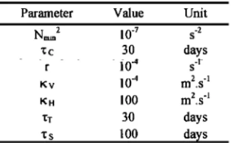
We impose restoring surface boundary conditions for temperature and salinity using the relaxation time constants Zr and Zs and the observed surface temperatures and salinities. The numerical implementation uses standard integration techniques. The model has 12 vertical layers down to 5000 m, the top layer being 100 m deep. There are 21 latitude bands. The model equations are given in the appendix, and the numerical values for the parameters are listed in Table 1.

In order to assess the ability of the model to reproduce the

main features of the thermohaline circulation, we first

performed an experiment with present-day surface boundary conditions. We used the Levitus [1982] temperature and salinity fields, averaged zonally over the Atlantic Ocean, as the prescribed surface forcing for our control experiment. A

crucial choice for such a two-dimensional model is the

definition of the averaging area in the deep water formation regions. Indeed, if we choose to average zonally the Arctic Ocean surface conditions, the resulting prescribed salinities in the high northern latitudes of the model will be much too low, because of the low salinities in the Bering Strait area of the Arctic Basin. In such a situation, the model cannot form deep

waters in the North Atlantic. It makes much more sense, from

an oceanographic point of view, to use only the Norwegian Sea sector of the Arctic Basin as our prescribed boundary

Table 1. Numerical Values of the Model

Parameters

Parameter Value model is a sector extending from 80øS to 90øN and 70 ø wide

in longitude.

The

bottom

is flat

at 5000

m depth.

Nmln

2

10

'7

Two-dim.•n•icm•!

oco.•n

models

have

been

used

recently

to

• c

1300.

investigate the stability of the thermohaline circulation r

[Hovine

and

Fichefet,

1994;

Marotzke

et al.,

1988;

Sakai

and

Kv

10

'4

Peltier,

1997;

Stocker

et al., 1992;

Thual

and McWilliams,

K,

100

1992;

Winton,

1997;

Wright

and Stocker,

1992]

and

also

to

•T

30

reconstruct

the

thermohaline

circulation

during

the

last

glacial

z s

100

Unit -2 s days -I s m2.s -1 m2.s -1 days days

718 PAILLARD AND CORTIJO' ATLANTIC MERIDIONAL CIRCULATION

1

80øS 60oS 30oS 0ON 30ON 60ON 90ON

Latitude

80ø'S' 6•øS''' :•0•'S ' ' ' 0ø'N .... •3•ø'N ''' 66ø'N ''' •6øN Latitude

80øS 60os 30os 0ON 30ON 60ON 90ON

Latitude 80'oS ' 6(•o s --30:S . . 0o, _Latitude N .... 36O.N-.. 66O'N-'' 90ON

Figure

1. (top)

temperature

and

(bottom)

salinity

annual

mean

fields

in the

model

for

the

control

run

(on

the

right)

compared

to the

Levitus

[1982] climatology (on the left). Contours are every IøC for temperature and every 0.29'oo for salinity.

conditions.

In this

area

(north

of 60øN),

we therefore

used

only

the 60øW-60øE sector of the ocean.

Similarly, Antarctic Bottom Waters (AABW) are formed in

extremely narrow regions, on the east side of the Antarctic

peninsula in the west part of the Weddell Sea, and also in the

west part of the Ross Sea. Using a global average of

temperatures and salinities all around Antarctica completely overrepresents regions were no deep water formation is

possible.

We therefore

made

our zonal

averaging

in only a 10

ø

longitude band around the deep water formation areas. It must

be emphasized

that these somewhat

arbitrary choices

are

crucial in determining the exact balance between NADW and AABW. This misrepresentation of the deep water formation regions is one of the major limitation of two-dimensional

oceanic models.

Using the wind stress from the Hellerman and Rosenstein

[1983] climatology, we have integrated the model from rest for at least 10,000 years, up to the equilibrium. The seasonal

cycle is explicitly resolved,

which is crucial for a good

representation of the high-latitude convection areas. The

resulting

annual mean temperature

and salinity fields are

compared

to the climatology

in Figure

1. We note the good

Levitus [1982] climatology. The annual mean overall meridional streamfunction is shown in Figure 2a: The NADW

and AABW strengths

are also in reasonable

agreement

with

current estimates [Macdonald and Wunsch, 1996], as are their

respective depths and extensions. The low-latitude wind-

driven

cells, in the upper

thermocline,

are superimposed

on

this general thermohaline circulation. The "no east-west

boundary

region"

in the Southern

Ocean

is also

driven

by the

upper wind stress,

and the induced

overturning

contributes

significantly to the interhemispheric water mass exchange

[Toggweiler and Samuels, 1993].

3. Past SST and SSS

Reconstruction

Accuracy

Since

we will investigate

in the following

the response

of

this model to paleoclimatic forcings, it is important to examine

the accuracy

of the available

data. SST are obtained

usually

from faunal assemblages, and the standard statistical estimates give an error of about 1 o to 2øC [Prell 1985]. The sea surface

salinities

(SSS) are estimated

using

the isotopic

composition

of planktic foraminifera. A careful error analysis shows that the main sources of uncertainty for these SSS estimates are the

SST values

and, to a smaller

extent,

the slope

of the $]80-

salinity regression [Cortijo et al., 1997; Schmidt, 1999]. In our

study,

we use

two extreme

cases

for the $]80-salinity

slope,

and the errors arise mainly from the SST errors. Indeed, a 2øC

error on SST may eventually lead to a 196o error on SSS, which is very important. However, it is then crucial to

understand how this may affect density, since the

thermohaline

circulation

is driven by density

gradients,

not

directly

by temperature

or salinity

gradients.

The error

analysis

must therefore go beyond a simple examination of SST and SSS errors. In particular, these errors are not independent and cannot be added like random errors. On the contrary, they mostly cancel out when computing density. Indeed, the two

statistically

independant

estimates

are the $]80 of calcite

and

the temperature.

If we use

a $]80-S

slope

of 2, we get the

following differential:

d•18Ocaco3

= d•518Omo

- 0.25

dT= 0.5 dS - 0.25

dT.

The differential

of density

is given

by dp = [3 dS - (x dT, with

(x and [3 being

the thermal

and

haline

expansion

coefficients.

This gives

dp= 2 [3

d•18Ocaco

3 + (0.5 [• - (g)

dT.

With [3 = 0.8 (%o-density/%o-salinity),

a = 0.3 (%o-density/øC)

for warm waters,

and ct = 0.1 (%o/øC)

for cold waters,

we get

Op/0T = 0.5 [3 - (x = 0.1%o/øC

for warm waters

and 0p/OT

PAILLARD AND CORTIJO: ATLANTIC MERIDIONAL CIRCULATION 719 o 2 3 0o/• .... 30•N 60•øN 90•ON I I I1• ,

'"'"",1

/

'

80o:• ' ' b0o'S .... 30o• .... 0oi•1 .... 3o•,N ' ' ' 6og N ' ' ' 90'ON 80o• ' ' 60'o S .... 30o• .... 0Ol•l .... 30•oN ' ' ' bO'•N ' ' ' 90'o N

Latitude Latitude

Figure 2. (a) Stream function obtained in the control run (contours every 2 Sv). The maximum of the North Atlantic Deep Water (NADW) overturning is 16.9 Sv at about 60øN, while the maximum of the Antarctic Bottom Water (AABW) is 13.2 Sv at 70øS. (b) The Last Glacial Maximum (LGM) experiment. The maximum of the NADW (or Glacial North Atlantic Intermediate Water (GNAIW)) overturning is 20.2 Sv at about 40øN, while the maximum of the AABW is 20.8 Sv always at 70øS. (c) Temperature and (d) salinity annual mean fields in the

model for the LGM run (contours every IøC and 0.2%0, respectively).

--0.3%o/øC for cold waters. This means that for a 2øC error on

the SST estimates, the corresponding density error will be between -- 0.2%0 and -- 0.6%0. This is considerably different from the independent accumulation of a 1%o error on salinity with a 2øC error on temperature. In particular, if CLIMAP [1981] is wrong at low latitudes, this has only a minor effect on the estimation of the density of seawater, since it depends

almost

entirely

on the estimation

8•80 of calcite

alone,

as also

noticed

by Lynch-Stieglitz

et al. [1999].

If we use a 8•80-

salinity slope of 1, the situation is even more favorable.

Indeed, we get 3o/3T = 0.25 [3- (• ---0.1%o/øC for warm

waters and 3o/3T -- +0.1%o/øC for cold waters. For a 2øC error on the SST estimates, the corresponding density error will always remain below 0.2%o.

If the errors on temperature and salinity reconstructions may be quite large, up to 2øC and up to 1%o, respectively, in

some cases, this translates into much smaller errors for the

density of seawater, between 0.2%0 and 0.6%0 in the worst

case. Since the thermohaline circulation results from large-

scale density gradients, and since the spatial coverage provided by the paleodata shows coherent large-scale

anomalies in SST and SSS, we believe it does make sense to

use paleotemperature and paleosalinity reconstructions as input of an ocean model to estimate the impact of sea surface changes on the deep ocean circulation.

estimated by CLIMAP [1981] for the temperatures and by Duplessy et al. [ 1991 ] and Wang et al. [ 1995] for the salinities. In the Southern Ocean, where no salinity reconstruction is yet available, we used a SSS anomaly equal to the global shift of +1.1%o, resulting from the about 120 m overall sea level lowering. Since the overall surface wind patterns remain the same during the LGM and since the influence of the wind stress is mostly limited to the upper thermocline ocean, we think that, in contrast to SST and SSS changes, wind stress changes will not affect significantly the general thermohaline structure. We are therefore using the present-day wind stress climatology as a surface boundary condition for the glacial ocean. The model is then integrated for several thousand years, up to the equilibrium. The resulting oceanic deep circulation is presented in Figure 2b, while the corresponding temperatures and salinities in the ocean interior are shown in Figures 2c and 2d. The circulation changes in this experiment are essentially located in the northern Atlantic. The deep water formation

occurs at lower latitudes, around 40ø-50øN instead of 60 ø-

70øN in the control run. The resulting NADW flow is also

much shallower and remains above 3000 m, and therefore

owes the new name of Glacial North Atlantic Intermediate

Waters (GNAIW) [Duplessy et al., 1988]. The Atlantic deep waters are therefore coming mainly from the south, even though the AABW flow remains almost unchanged at about 2

4. The Last Glacial Maximum Experiment

In order to investigate the role of temperature and salinity changes on the oceanic circulation during the Last Glacial Maximum (LGM), we performed an experiment where the

SST and SSS fields are relaxed to their LGM values, as

to3 Sv. The ocean bottom waters cool by about 1 øC as a result

of the greater extent of the cold AABW contribution. For the same reason, the bottom waters are also fresher by about 0.1%o, in addition to the global +1.1%o shift. Conversely, since the North Atlantic waters are sinking at lower latitudes, the temperatures around 2000 m are slightly warmer in the LGM experiment than during the control run.

720 PAILLARD AND CORTIJO: ATLANTIC MERIDIONAL CIRCULATION

The pattern of a shallower and southward shifted NADW

(or GNAIW) flow is consistent

with •5•3C

and A•4C

this time. Indeed, deep waters in the Atlantic Ocean are

systematically

depleted

in •4C

and

enriched

in •3C

during

the

intermediate waters, above 2500 m, exhibit the opposite

changes [Duplessy et al., 1988], which indicates a possibly better than present intermediate water ventilation. Previous

experiments

with a two-dimensionnal

(2-D) ocean model

forced by reconstructed SST and SSS for the LGM [Fichefet et al., 1994] have shown the same general southward shift of the

deep

water

formation

area

and the same

shallower

sinking

of

these waters. However, in contrast to our results, the NADW

(or GNAIW) strength was significantly weaker in the LGM run than in the control run. This probably results from slight differences in model configuration near the deep water

formation areas. In particular, their top level is only 50m deep

instead of 100m here. We believe 100 m is more

representative of what the foraminiferal assemblages are able

to record in terms of anomalous SST and SSS.

A coupled ocean-atmosphere simulation has also been performed for this time period [Ganopolski et al., 1998], where a 2-D ocean was coupled to a simplified atmospheric

circulation model. In this simulation where LGM SST and

SSS fields are not used as input, the corresponding NADW strength is very similar to the control run. This result is quite comparable to our results. The corresponding depth and location of the deep water formation are also very similar to our findings. In contrast, another LGM simulation, using a 3-D ocean model coupled to an energy and moisture balance model [Weaver et al., 1998], exhibits a much reduced and much deeper NADW formation, without significant changes in the location of the deep water formation area, together with an almost complete wanishing of AABW, in contradiction to paleoceanographic data. However, in contrast to the Ganopolski et al. model, water vapor is diffused, not advected, in the atmosphere. This may lead to quite unrealistic precipitation patterns and probably has some strong influence on the resulting thermohaline circulation.

Both the comparison of the control run with the climatology and the quite reasonable results obtained for the LGM experiment make us confident that our simplified ocean model is suitable for simulating the state of the Atlantic Ocean before and during a Heinrich event, using the available SST and SSS

data.

5. The Heinrich Event 4 Experiments

The reconstructed SST and SSS anomalies [Cortijo et al., 1997] are shown in Figure 3. The methodology used to obtain these fields is strictly similar to the one used for the LGM. In particular, it is possible to reconstruct both winter and summer SSTs and thus to have an idea of the seasonal cycle for temperature. However, the reconstructed SSS anomaly fields are assumed to be annual mean values, and the salinity seasonal cycle remains therefore identical to the present-day one. This may represent a significant limitation of the method, since the high-latitude convection is mainly seasonal and depends strongly on the surface salinity fields. Nevertheless,

0 • g-3 E -4 -5 • 0 E •-1 • '•-2 '• -4 -5 35

[

•[ "' ""-• : slopeS/15

O l

Figure 3. Summary of the Heinrich event 4 (HE 4) surface hydrological perturbation [from Cortijo et al., 1997]. The differences in summer sea surface temperature and surface salinity during HE 4 and before the event are plotted here to emphasize the cooling (between 3 ø and 4øC) and the

freshening (between 1 and 3960, depending on the choice of b•80-S slope)

in the iceberg melting area.

for the HE 4 experiments, the major limitation comes from the very restricted area where such surface hydrological

reconstructions are available. Indeed, the model needs a full

SST and SSS coverage of the Atlantic Ocean as boundary conditions, whereas these fields are available only in the 40øN-60øN latitude band for time slices around HE 4. A major

difficulty in extending this data coverage southward concerns the precise dating and correlation of paleoclimatic proxies

accross the whole Atlantic Ocean. If such a correlation is

possible

in the vicinity of the iceberg

melting

area, with the

clear identification of the ice-rafted debris defining Heinrich

layers, the problem is much more difficult for more southern

sediment cores.

We decided to use the available data together with the LGM

boundary conditions in order to run the model. The following HE 4 experiments are therefore perturbation experiments,

around the LGM state, to changes in the hydrological properties of the surface ocean near the iceberg melting area. The data are indeed available precisely in this area, where the icebergs associated with the Heinrich events are melting and depositing their debris to the sediment, but this latitude band is also the area where the LGM North Atlantic Deep Water (or GNAIW) forms. We can therefore experiment, with our simplified model, how the SST and SSS changes in this

critical area affect the overall thermohaline circulation pattern.

We have performed three experiments. The first one uses the reconstructed SST and SSS just before the Heinrich event. The situation during the event corresponds to the second

experiment,

assuming

that

the •5•80-salinity

relationship

is 1:1,

which assumes that the surface salinity decrease is due only to

the meltwater from the ice sheets, in the same fashion as the

global glacial-interglacial transitions [Fairbanks, 1989]. The third experiment is also for the HE 4 event, assuming that the

•5•80-salinity

relationship

is 1:2. This is the present-day

relationship observed for surface ocean waters, which results from the evaporation and precipitation processes [Craig and Gordon, 1965]. For each of these experiments, the model is integrated for 3000 years, up to the equilibrium. It is worth

PAILLARD AND CORTIJO: ATLANTIC MERIDIONAL CIRCULATION 721

80• '•' ' -j0• --- a• - - - j&ff--•"

•' •!

• '1•-

•- '

I

Lati•de Latitude Latitude

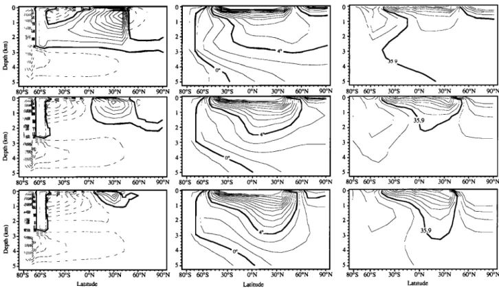
Figure

4. (top)

Before

HE

4. (middle)

During

HE

4, with

•80-S slope

= 1. (bottom)

During

HE

4, with

fi•80-S

slope

= 2. (right)

Stream

functions (contours eveff 2 Sv). Maximum of clockwise flow: (top) 21.5 Sv, (middle) 11.2 Sv, (bosom) 9.0 Sv. Maximum of •BW: (top) 19.4 Sv, (middle) 31.6 Sv, (bosom) 33.3 Sv. (middle) Temperatures (contours eveff loC). (le•) Salinities (contours eveff 0.2%0).

noticing that an Heinrich event lasts probably much less than 3000 years, and these experiments cannot pretend to reproduce exactly what happens during HE 4. Nevertheless, after a few hundred years of model integration, the North Atlantic circulation is very close to its equilibrium state. The results shown hereafter are therefore representative of a Heinrich

event which would last at least several hundred years, which is

a reasonable assumption [Francois and Bacon, 1994]. The

data used for the SST and SSS are actually averages on a time

period

of the order

of 1000 years.

It is therefore

quite

sensible

to look at the equilibrium response of the ocean to SST and

SSS changes. These results are shown in Figure 4.

Since the reconstructed temperatures and salinities just

before the event. are only sligthly different from their LGM

values, this first experiment is a small perturbation of the

LGM state obtained before. The results are therefore not

significantly different from the LGM ones. On the contrary,

the SST and SSS are considerably lowered during the event, and the thermohaline circulation obtained by the model is

notably affected. The reduction of North Atlantic Deep Water

formation is such that there is, in our model, no more outflow

of NADW from the North Atlantic to the south and,

6. Discussion

The collapse of the thermohaline circulation in the North Atlantic during Heinrich event 4 obtained in our numerical experiments is entirely consistent with the results of Vidal et

al. [1997],

which

have

demonstrated

that the 8•3C

of the

benthic foraminifera, living in the deep sea at this time, was

considerably depleted during each Heinrich event, thus suggesting a much reduced deep water ventilation. Such a reduction is also expected in order to account for the considerable cooling observed in ice core records at these times [Dansgaard et al., 1993]. Indeed, as already mentioned in section 1, the Atlantic Ocean transports northward a

considerable amount of heat. A reduction or a collapse of the

thermohaline circulation is therefore probably the best

explanation

for the recorded

coolings

in Greenland.

We have

plotted,

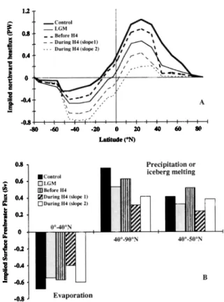
in Figure 5a, the Atlantic northward

heat fluxes

obtained from our experiments. As expected, the heat transport

during HE 4 is much reduced. It is also interesting to note

from Figure 5 that, though the LGM experiment overturning is stronger than the control one, the LGM oceanic heat transport

is much smaller. This is due mainly to the more southerly

consequently,

to other basins. Since the near-surface location

of deep

water

formation

during

LGM, which

therefore

overturning is controlled in a large part by the wind stress, the results presented here suggest a nearly complete collapse of the circulation during Heinrich event 4. This collapse is even

more evident when the 1:2 slope is used for salinity

reconstructions. Since the deep waters are now fueled only by the southern flow, the deep North Atlantic is even cooler and

fresher than it was in the LGM experiment.

considerably reduces the efficiency of meridional heat transport. This heat transport is somewhat larger before HE 4 than during LGM, which is also consistent with the higher temperatures recorded during marine isotopic stage 3. The interhemispheric heat transport is northward for the control, the LGM, and the "before HE 4" experiments, while it

722 PAILLARD AND CORTIJO: ATLANTIC MERIDIONAL CIRCULATION 1.2 0.s 0.4 0 -0.8 -80 ..-- Control • LGM _ . Before H4 During H4 (slopel) -. - During H4 (slope 2) . oO

ß

A

Figure 5. (a) The northward oceanic heat transport for the five numerical experiments. The maximum Northern Hemisphere values are, for the

control run, 1.04 PW; for the LGM, 0.65 PW; before HE 4, 0.87 PW;

during HE 4 (slope = 1), 0.43 PW; and during HE 4 (slope = 2), 0.20 PW. (b) The implied surface freshwater fluxes for different latitude bands: between 0 ø and 40øN, where evaporation dominates; between 40 ø and 90øN, where precipitation dominates; and the iceberg meltwater band between 40 ø and 50øN. In this last area, the freshwater fluxes required to maintain the equilibrium are not larger during HE 4 than they were before

HE 4.

with the warming observed in Antarctica during the cold

phases of the northern North Atlantic associated with Heinrich

events [Blunier et al., 1998].

We must nevertheless keep in mind that our HE 4

experiments are actually perturbation experiments around the

LGM state of the Atlantic Ocean, since the coverage of SST and SSS reconstructions is limited to the high latitudes of the Atlantic. It may be possible that SST and SSS in the equatorial and south Atlantic are, before and during a Heinrich event, different from their LGM values. Nevertheless, if the deep

water formation in the North Atlantic before a Heinrich event

is in the 40ø-50øN latitude band as is the case at LGM, then

the decrease

in salinity reconstructed

from the 5•SO

measurements during HE 4 is such that the collapse of the thermohaline circulation is probably inevitable, as suggested by our model.

With our ocean model, it is also quite straightforward to

compute the surface freshwater fluxes required to maintain the equilibrium. These fluxes are plotted in Figure 5b for the low and high latitudes of the North Atlantic. We note that the evaporation at low latitudes and precipitation at high latitudes

is reduced during the LGM compared to the control run, which

is expected for a climate much cooler and therefore drier than today. More surprisingly, these required freshwater fluxes are _

also smaller during the Heinrich event (Figure 5b), which seems to contradict the considerable freshening recording by the SSS data and caused by the iceberg discharge. First, there is no reason to think that, during an Heinrich event, the meltwater flux at high latitude is compensated by evaporation at lower latitude. In other words, during a real Heinrich event, the water budget of the ocean is probably not equilibrated. The equilibrium freshwater fluxes shown in Figure 5b have therefore a quite limited relevance to the Heinrich event situation. Nevertheless, it is interesting to note that, when the Atlantic thermohaline circulation is greatly reduced, or even

collapsed, the freshwater flux at high latitude required to

maintain this state is quite low. This probably results from the hysteresis phenomena associated with the thermohaline multiple equilibria [Rahmstorf, 1995; Stommel, 1961]: Once

the advective circulation is shut down by a freshwater input, it

can stay down even when the freshwater input vanishes. Of course, the stability of the equilibrium states found in our

study needs to be investigated with a more complex, coupled

ocean-atmosphere model, and, ultimately, the understanding

of the physics of Heinrich events requires a detailed modelling of the ocean, atmosphere, and ice sheet freshwater budgets.

7. Conclusion

We have performed numerical experiments, with a simplified two-dimensionnal ocean model, in order to better

understand the physical consequences, on the deep ocean circulation, of the recorded North Atlantic surface cooling and freshening during a Heinrich event. In contrast to previous studies, we made no assumption about freshwater input. The

main limitation of our experiments comes from the limited

availability of detailed quantitative sea surface temperature and salinity reconstructions for such critical time periods.

Assuming that the ocean state outside the North Atlantic is

similar to the LGM situation, we have shown that the

reconstructed SST and SSS for the HE 4 time period are strongly suggesting a nearly complete collapse of the North

Atlantic thermohaline circulation. This result is consistent with

records of the deep sea ventilation during Heinrich events, like

the $•3C

of benthic

foraminifera.

Such

a collapse

has

been

predicted by many authors [Manabe and Stouffer, 1993;

Rahmstorf and Ganopolski, 1998; Stocker and Schmitther,

1997] in the context of future, greenhouse-induced, global

warming. It would therefore be of great value to better

constrain the thresholds on thermal and haline forcing, beyond which such a collapse will inevitably occurs. A detailed

reconstruction of the climatic conditions around a Heinrich

event like HE 4 could be extremely helpful in assessing the

odds of such an eventuality.

Appendix: Model Equations

In the real ocean, the main dynamical balance is essentially the geostrophic one: The Coriolis force balances the pressure

gradient one:

1 3p

f0 sin0 v-- •

• + (higher

- order

terms),

(1)

P0Rcos0

32

where f0 is-the Coriolis parameter, 0 is the latitude, v is the meridional velocity, P0 is the mean seawater density, R is the

PAILLARD AND CORTIJO' ATLANTIC MERIDIONAL CIRCULATION 723

radius

of the Earth,/T

is the longitude,

and p is he pressure.

In

a two-dimensional model, it is impossible to represent

explicitly

the zonal

gradients.

We need

a new

equation

that

relates the meridional velocity v to the merional pressure

gradient/)p/a0.

Two

main

different

approaches

have

been

used

so far. The first is neglecting

the rotation

of the Earth

and

replacing

the geostrophic

balance

with a dissipative

one

[Marotzke

et al., 1988;

Sakai

and

Peltier,

1997;

Thual

and

McWilliams,

1992;

Winton,

1997].

The alternative,

introduced

by Wright

and Stocker

[1991], is to assume

that the mean

zonal

pressure

gradient/)p/aX

is proportional

to the meridional

one,/)p/a0.

We are using

the Winton

[1997]

parameterization,

which is, to first order, equivalent to the more sophisticated

Wright

and

Stocker

approach.

The model

equations

are:

-1 cgp F w

v - + , (2)

rP0R

c•0 f0sin0

where

r is the

ad hoc

Rayleigh

damping

coefficient

(in s

'•) and

where

Fw is a force

applied

only in the top level

of the model,

to account for the wind forcing:

r W

PO•E

(3)

in which

Zw is the zonal

wind stress

and

8 E is the thickness

of

the top layer of the model.

Since there are no east or west boundaries in the Southern

Ocean,

at least

in the top 2000 or 3000 m, there

can be no

zonal pressure

gradient,

and therefore

the geostrophic

meridional

velocity

must

vanish.

This is taken

into account

by

setting

the Rayleigh

coefficient

r to infinity.

The vertical

velocity

w is obtained

from

the mass

balance

equation,

the

pressure

p is given

by the

hydrostatic

equation,

and

the

density

p is computed

as a function

of T (in Celsius)

and

S (in permil)

using

a third-order

polynomial

approximation

[Cox et al.,

1970].

We use

the rigid

lid approximation

at the surface

of the

model.

The evolution

equations

for the temperature

and salinity

+(c

+tCV)

ø•2T

oqz

2 •I '

--+V--•

3t R 30

+ w-- = tc

o•z

H

R 2cos

0 c)

0

cos0

c)2S

(

)--+F (S)

(4b)

+ c + tc

V o•z

2 S '

where FT(T) and Fs(S) are the surface temperature and salinity forcings, null in the ocean interior and equal to the following

at the surface:

FT(T)

= (T-TR), Fs(S)

= --

S

R ,

r T r s

in which ZT and Zs are the relaxation time constants and TR and

SR are the observed surface temperatures and salinities. In equations (4a) and (4b), •CH and •c v are the horizontal and vertical eddy diffusivity. The variable c is the contribution of vertical convective mixing to vertical diffusivity. Following [Schmidt and Mysak, 1996], we use the formula below for c:

I 1-tanh(

c + tc v = tc v , (6)

where N is the Brunt-V•iis•il•i frequency:

N2

= __•_g

0/9

P0 3z

N mi n is the marginaly stable value of N, and •c is the enhanced vertical diffusivity in the fhlly convective regime. This last parameter can also be written

2

Az

max (8)

K C = ,

r C

where Azma x is the largest ve•ical grid spacing and Zc is a

characteristic time for ve•ical convection.

The numerical implementation uses standard integration techniques. The model has 12 ve•ical layers. The base of each layer lies at the following depths: 100, 300, 600, 1000, 1500,

2000, 2500, 3000, 3500, 4000, 4500, and 5000 m. There are

21 latitude bands positioned between the following latitudes:

80øS, 70øS, 65øS, 60øS, 55øS, 50øS, 40øS, 30øS, 20øS, 10øS, 5øS, 0øN, 5øN, 10øN, 20øN, 30øN, 40øN, 50øN, 60øN, 70øN, 80øN, and 90øN. The numerical values for the different

parameters are given in Table 1.

Acknowledgments. Basic support from CEA and CNRS to the

LSCE and from PNEDC and the EU Environment program ENV4-

CT97-0643 is acknowledged. This paper greatly benefited from the

comments of J.C. Duplessy and three anonymous reviewers. Part of

this work was performed when D. Paillard was visiting NCAR with

support from NATO. This is LSCE contribution 305A.

References

Blunier, T., et al., Asynchrony of Antarctic and sediments and Greenland ice, Nature, 365, 143- structions of the Earth's Surface at the Last Greenland climate change during the last glacial 147, 1993. Glacial Maximum, Map and Chart Series//36, period, Nature, 394, 739-743, 1998. Broecker, W.S., D.M. Peteet, and D. Rind, Does the Geol. Soc. of Am, Boulder, Colo., 1981. Bond, G., et al., Evidence of massive discharges of ocean-atmosphere system have more than one Cortijo, E., P. Yiou, L. Labeyrie, and M. Cremer,

icebergs into the North Atlantic Ocean during mode of operation?, Nature, 315, 21-26, 1985. Sedimentary record of rapid climatic variability the last glacial period, Nature, 360, 245-249, Bryan, F., High-latitude salinity effects and in the North Atlantic Ocean during the last

1992. interhemispheric thermohaline circulations, glacial cycle, Paleoceanography, 10, 911-926,

Bond, G., W. Broecker, S. Johnsen, J. McManus, L. Nature, 323, 301-304, 1986. 1995.

Labeyrie, J. Jouzel, and G. Bonani, Correlations Climate' Long-Range Investigation, Mapping, and Cortijo, E., L. Labeyrie, L. Vidal, M. Vautravers,

724 PAILLARD AND CORTIJO: ATLANTIC MERIDIONAL CIRCULATION

Arnold, J.-L. Turon, and G. Auffret, Changes in

sea surface hydrology associated with Heinrich

event 4 in the North Atlantic Ocean between

40øN and 60øN, Earth Planet. Sci. Lett., 146, 29-45, 1997.

Cox, R.A., M.J. McCartney, and F. Culkin, The

specific gravity/salinity/temperature relationship in natural sea water, Deep Sea Res. Oceanogr.

Abstr., 17, 679-689, 1970.

Craig, H., and L.I. Gordon, Deuterium and oxygen

18 variations in the ocean and the marine

atmosphere: Stable isotopes in oceanographic studies and paleotemperatures, in Proceedings

of the Third Spoleto Conference, Spoleto, Italy,

edited by E. Tongiorgi, pp. 9-130, Sischi and

Figli, Pisa, Italy, 1965.

Dansgaard, W., H.B. Clausen, N. Gundestrup, C.U.

Hammer, S.J. Johnsen, P.M. Kristinsdottir, and N. Reeh, A new Greenland deep ice core,

Science, 218, 1273-1277, 1982.

Dansgaard, W., et al., Evidence for general instability of past climate from a 250-kyr ice-

core record, Nature, 364, 218-220, 1993.

Duplessy, J.C., N.J. Shackleton, R.G. Fairbanks, L.D. Labeyrie, D. Oppo, and N. Kallel, Deepwater source variations during the last climatic cycle and their impact on the global

deepwater circulation, Paleoceanography, 3,

343-360, 1988.

Duplessy, J.-C., L. Labeyrie, A. Juillet-Leclerc, F.

Maitre, J. Duprat, and M. Sarnthein, Surface salinity reconstruction of the North Atlantic

Ocean during the last glacial maximum,

Oceanol. Acta, 14, 311-324, 1991.

Fairbanks, R.G., A 17,000 year glacio-eustatic sea level record: Influence of glacial melting rates on the Younger Dryas event and deep ocean

circulation, Nature, 342, 637-642, 1989.

Fichefet, T., S. Hovine, and J.-C. Duplessy, A model study of the Atlantic thermohaline

circulation during the last glacial maximum,

Nature, 372, 252-255, 1994.

Franqois, R., and M.P. Bacon, Heinrich events in

the North Atlantic: Radiochemical evidence,

Deep Sea Res., Part 1, 41, 315-334, 1994.

Ganopolski, A., S. Rahmstorf, V. Petoukhov, and M. Claussen, Simulation of modem and glacial climates with a coupled global model of intermediate complexity, Nature, 391, 351-356,

1998.

Heinrich, H., Origin and consequences of cyclic ice

rafting in the northeast Atlantic Ocean during

the past 130,000 years, Quat. Res., 29, 142-152,

1988.

Hellerman, S., and M. Rosenstein, Normal monthly

wind stress over the world ocean with error

estimates, d. Phys. Oceanogr., 13, 1093-1104,

1983.

Hovine, S., and T. Fichefet, A zonally averaged,

three-basin ocean circulation model for climate

studies, Clim. Dyn., 10, 313-331, 1994.

Levitus, S., Climatological Atlas of the World Ocean, Prof Pap. No. 13, Natl. Oceanic and Atmos. Admin., U.S. Govt. Print. Off.,

Washington, D.C., 1982.

Lynch-Stieglitz, J., W.B. Curry, and N. Slowey, A

geostrophic transport estimate for the Florida

Current from the oxygen isotope composition of benthic foraminifera, Paleoceanography, 14,

360-373, 1999.

MacAyeal, D.R., A low-order model of the

Heinrich event cycle, Paleoceanography, 8,

767-773, 1993.

Macdonald, A.M., and C. Wunsch, An estimate of Stocker, T.F., and D.G. Wright, Rapid changes ir. global ocean circulation and heat fluxes, Nature, ocean circulation and atmospheric radiocarbon,

382, 436-439, 1996. Paleoceanography, 11, 773-795, 1996.

Maier-Reimer, E., and U. Mikolajewicz, Stocker, T.F., D.G. Wright, and W.S. Broecker, The Experiments with an OGCM on the cause of the influence of high-latitude surface forcing on the

Younger-Dryas, Tech. Rep. 39, pp. 1-13, Max- global thermohaline circulation,

Planck-Inst. far Meteorol., Hamburg, Germany, Paleoceanography, 7, 529-541, 1992.

1989. Stommel, H.M., Thermohaline convection with two

Manabe, S,, and R.J. Stouffer, Century-scale effects stable regimes of flow, Tellus, 13, 224-230,

of increased atmospheric CO2 on the ocean- 1961.

atmosphere system, Nature, 364, 215-218, 1993. Thual, O., and J.C. McWilliams, The catastrophic Manabe, S., and R.J. Stouffer, Simulation of abrupt structure of thermohaline convection in a two-

climate change induced by freshwater input to dimensional fluid model and a comparison with

the north Atlantic ocean, Nature, 378, 165-167, low-order box model, Geophys. Astrophys.

1995. Fluid Dyn., 64, 67-95, 1992.

Marotzke, J., P. Welander, and J. Willebrand, Toggweiler, J.R., and B. Samuels, Is the magnitude

Instability and multiple steady states in a of the deep outflow from the Atlantic Ocean

meridional-plane model of the thermohaline

circulation, Tellus, Ser. A, 40, 162-172, 1988.

Mikolajewicz U., T.J. Crowley, Schiller A. and R.

Voss, Modelling teleconnections between the

North Atlantic and North Pacific during the

Younger Dryas, Nature, 387, 384-387, 1997.

Oerlemans, J., A numerical study on cyclic

behaviour of polar ice sheets, Tellus, Ser. A, 35,

81-87, 1983.

Paillard, D., The hierarchical structure of glacial

climatic oscillations: interactions between ice-

sheet dynamic and climate, Clint. Dyn., 11, 162-

177, 1995.

Paillard, D., and L. Labeyrie, Role of the thermohaline circulation in the abrupt climate warming after Heinrich events, Nature, 372,

162-164, 1994.

Prell, W.L., The stability of low-latitude sea-surface

temperatures: An evaluation of the CLIMAP

reconstruction with emphasis on the positive

SST anomalies, Rep. TR 025, U.S. Dep. of

Energy, Washington, D.C., 1985.

Quon, C., and M. Ghil, Multiple equilibria and

stable oscillations in thermosolutal convection

at small aspect ratio, J. Fluid Mech., 245, 449-

483, 1995.

Rahmstorf, S., Bifurcations of the Atlantic thermohaline circulation in response to changes

in the hydrological cycle, Nature, 378, 145-149,

1995.

Rahmstorf, S., and A. Ganopolski, Long-term global warming scenarios computed with an

efficient coupled climate model, Clint. Change,

43, 353-367, 1998.

Sakai, K., and W.R. Peltier, A multi-basin reduced

model of the global thermohaline circulation:

Paleoceanographic analyses of the origins of ice-age climate variability, J. Geophys. Res.,

101, 22,535-22,562, 1996.

Sakai, K., and W.R. Peltier, Dansgaard-Oeschger

oscillations in a coupled annosphere-ocean

climate model, J.. Clint., 10, 949-970, 1997.

Schmidt, G.A., Error analysis of paleosalinity calculations, Paleoceanography, 14, 422-429,

1999.

Schmidt, G.A., and L.A. Mysak, The stability of a

zonally averaged thermohaline circulation

model, Tellus, Ser. A, 48, 158-178, 1996.

Stocker, T.F., and A. Schmittner, Influence of CO2 emission rates on the stability of the thermohaline circulation, Nature, 388, 862-865,

1997.

Stocker, T.F., and D.G. Wright, Rapid transitions of

the ocean's deep circulation induced by changes

in surface water fluxes, Nature, 351, 729-732,

1991.

actually governed by Southern Hemisphere winds?, in The Global Carbon Cycle, edited by

M. Heimann, NATO ASI Ser., Ser. I,, 303-331, 1993.

Vidal, L., L. Labeyrie, E. Cortijo, M. Arnold, J.-C

Duplessy, E. Michel, S. Becqu6, and T.C.E. van

Weering, Evidence for changes in the North

Atlantic deep water linked to meltwater surges

during the Heinrich events, Earth Planet. Sci.

œett., 146, 13-27, 1997.

Wang, L., M. Sarnthein, J.-C. Duplessy, H.

Erlenkeuser, S. Jung, and U. Pflaumann, Paleo

sea surface salinities in the low-latitude

Atlantic: The •180 record of Globigerinoides

ruber (white), Paleoceanography, 10, 749-761,

1995.

Weaver, A.J., M Eby, A.F. Fanning, and E.C. Wiebe, Simulated influence of carbon dioxide,

orbital forcing and ice sheets on the climate of

the Last Glacial Maximum, Nature, 394, 847-

853, 1998.

Winton, M., The effect of cold climate upon North Atlantic deep water formation in a simple

ocean-atmosphere model, J. Clint., 10, 37-51,

1997.

Winton, M., and E.S. Sarachik, Thermohaline

oscillations induced by strong steady salinity

forcing of ocean general circulation models, J. Phys. Oceanogr., 23, 1389-1410, 1993.

Wright, D.G., and T.F. Stocker, A zonally averaged

ocean model for the thermohaline circulation, I, Model development and flow dynamics, J. Phys. Oceanogr., 21, 1713-1724, 1991. Wright, D.G., and T.F. Stocker, Sensitivities of a

zonally averaged global ocean circulation model, J. Geophys. Res., 97, 12,707-12,730,

1992.

Zhang, S., R.J. Greatbatch, and C.A. Lin, A

reexamination of the polar halocline catastrophe

and implications for coupled ocean-atmosphere

modeling, J. Phys. Oceanogr., 23, 287-299,

1993.

E. Cortijo and D. Paillard, Laboratoire des

Sciences du Climat etde l'Environnement, Centre d'Etudes de Saclay, Orme des M•isiers, 91191 Gif sur Yvette, France. (paillar•lsce.saclay.cea. fr)

(Received March 24, i999;

revised July 13. 1999;