HAL Id: hal-01738266
https://hal-ifp.archives-ouvertes.fr/hal-01738266
Submitted on 20 Mar 2018HAL is a multi-disciplinary open access
archive for the deposit and dissemination of sci-entific research documents, whether they are pub-lished or not. The documents may come from teaching and research institutions in France or abroad, or from public or private research centers.
L’archive ouverte pluridisciplinaire HAL, est destinée au dépôt et à la diffusion de documents scientifiques de niveau recherche, publiés ou non, émanant des établissements d’enseignement et de recherche français ou étrangers, des laboratoires publics ou privés.
A continuum voxel approach to model flow in 3D fault
networks: a new way to obtain up-scaled hydraulic
conductivity tensors of grid cells
André Fourno, Christophe Grenier, Abdelhakim Benabderrahmane, Frédérick
Delay
To cite this version:
André Fourno, Christophe Grenier, Abdelhakim Benabderrahmane, Frédérick Delay. A contin-uum voxel approach to model flow in 3D fault networks: a new way to obtain up-scaled hy-draulic conductivity tensors of grid cells. Journal of Hydrology, Elsevier, 2013, 493, pp.68-80. �10.1016/j.jhydrol.2013.04.010�. �hal-01738266�
1
A continuum voxel approach to model flow in 3D fault networks: a new way to
1
obtain up-scaled hydraulic conductivity tensors of grid cells
2
André Fourno1, Christophe Grenier2, Abdelhakim Benabderrahmane3, Frederick Delay4.
3
1
Corresponding author, IFP Energies Nouvelles, 1&4 Avenue du Bois Préau 92500 Rueil-4
Malmaison, France. Tel.:+33 1 47 52 72 57. Fax:+33 1 47 52 60 31. 5
andre.fourno@ifpenergiesnouvelles.fr
6
2
Laboratoire des Sciences du Climat et de l'Environnement UMR 8212 CNRS-CEA-UVSQ, 7
CEA/Orme des Merisiers 91191 Gif-sur-Yvette Cedex, France. 8
3
ANDRA, DRD/EAP, Parc de la Croix Blanche, 1-7 rue Jean Monnet, 92298 Châtenay-Malabry, 9
France. 10
4
LHyGeS - UMR CNRS 7517. 1, Rue Blessig 67084 Strasbourg cedex, France. 11
12
Abstract
13 14
Modelling transfers in fractured media remains a challenging task due to the complexity of the 15
system geometry, high contrasts and large uncertainties on flow and transport properties. In the 16
literature, fractures are classically modelled by equivalent properties or are explicitly represented. 17
The new Fracture Continuum Voxel Approach (FCVA), is a continuum approach partly able to 18
represent fracture as discrete objects; the geometry of each fracture is represented on a regular 19
meshing associated with a heterogeneous field of equivalent flow properties. The mesh-20
identification approach is presented for a regular grid. The derivation of equivalent voxel 21
parameters is developed for flow simulated with a Mixed Hybrid Finite Element (MHFE) 22
scheme. The FCVA is finally validated and qualified against some reference cases. The resulting 23
method investigates multi-scaled fracture networks: a small scale homogenized by classical 24
methods and large discrete objects as that handled in the present work. 25
26
Highlights
27
• An accurate mapping of discrete fracture networks onto a regular mesh is obtained 28
2
• A full hydraulic conductivity tensor in each mesh is needed to model fracture fluxes 29
• hydraulic properties preserve continuity of fluxes between neighbouring meshes 30
• Various hydraulic behaviour at fracture intersections can be modelled 31
32
Keywords
33
Fractured media, Up-scaling, Equivalent hydraulic conductivity tensors, Mixed hybrid finite 34 elements. 35 36
1 Introduction
37Within the research community involved in the studies of transfers in fractured media, special 38
emphasis is regularly put on experimentation and simulation of flow and transport in fractured 39
media for various reasons, e.g., prediction of oil production (Bourbiaux, 2010), improvement of 40
storage capacity for gas (Iding and Ringrose 2009; Ringrose et al., 2011), safety assessment of 41
nuclear waste repositories (Geotrap, 20002; Chapman and McCombie, 2003) etc. Several 42
constraints make this modelling work a challenging task: the geometrical complexity of the 43
system, the scarcity of available data, and the strong contrasts in parameter values between 44
mobile and immobile zones (Bear et al., 1993; Neuman, 2005). 45
46
Transfers in fractured media have already been subjected to intense modelling work (e.g., Bear et 47
al., 1993; Koudina et al., 1998; Berkowitz, 2002; Bogdanov et al., 2003; Karimi-Fard et al., 2004; 48
Adler et al., 2005). A large diversity of models exists, with differences on both the fracture 49
medium conceptualization and the way to represent physically and numerically the flow and 50
transport mechanisms. These differences make comparisons of the approaches a complex task 51
(Selroos et al., 2001). For spatially distributed models relying on Eulerian approaches to flow 52
and transport, the meshed representation of the fracture medium is the first difficulty to 53
overcome. The fracture network geometry can be explicitly accounted for or replaced by 54
equivalent properties mapped onto a regular or irregular (geological) grid mesh. It is then referred 55
to the so-called discrete and continuous approaches, respectively. 56
For discrete approaches, fractures are often modelled by means of planar objects (e.g., Cacas et 57
al., 1990; Dershowitz et al., 1991; Cvetkovic et al., 2004; Adler et al., 2005; Pichot et al., 2010; 58
3
de Dreuzy et al., 2012; Noetinger and Jarrige, 2012; for Discrete Fracture Network approaches) 59
or linear objects with the consequence of limiting flow to channels within fracture planes and at 60
fracture intersections (channel models or pipe network models, Dverstorp et al., 1992; Moreno 61
and Neretnieks, 1993; Tsang and Neretnieks, 1998; Ubertosi et al., 2007). Nevertheless, specific 62
meshing efforts are required which become cumbersome when a large number of fractures has to 63
be represented, for instance with small scale fractures. Some attempts however based on corner-64
point grids and finite-volume approaches mixing two-dimensional and one-dimensional elements 65
for fracture planes and fracture intersections, respectively are able to partly homogenize complex 66
fracture fields (Karimi-Fard et al., 2006). 67
68
On the other hand, the so-called continuous approaches are commonly used in petroleum 69
engineering and hydrology for simulating reservoirs especially when the latter are of sedimentary 70
type. As suggested by their name, the classical single continuum approaches consider a single 71
equation to cope with flow in both fractures and matrix. However, fractured rocks are often 72
depicted by two (or more) media with contrasted properties, for example, to separate the fracture 73
network from the matrix medium. The subsequent dual-continuum approaches (Barrenblatt et al. 74
1960; Warren and Root, 1963; Delay et al., 2007) deal with one equation of flow in each medium 75
and an additional term of transfer between the two media for closing the problem (see the 76
extended review of existing approaches in Berkowitz, 2002). According to the degree of 77
complexity introduced in the system, the resolution of flow can either be performed numerically 78
in both media, or the incidence of matrix on flow in fractures is handled by means of analytical 79
solutions (Grenier and Benet, 2002). Continuous approaches rely upon the definition of a 80
Representative Elementary Volume (REV), defined for instance as the minimal block size for 81
which the mean hydraulic conductivity value stabilizes when increasing the size of the block 82
(Long et al., 1982). At the REV scale, it becomes possible to calculate equivalent hydraulic 83
properties that take into account the presence of fractures. Unfortunately, the REV does not 84
always exist, as with the cases of poorly connected fracture networks (e.g., fracture network at 85
the percolation threshold) or networks of large faults with characteristic lengths of the same order 86
as the size of the investigated domain. The equivalent properties (e.g., hydraulic permeability for 87
flow resolution) may be obtained analytically (Oda, 1985, 1986; Lee et al., 1995; Pan et al., 88
2010) or numerically (Bourbiaux et al., 1998; Koudina et al., 1998; Delorme et al., 2008) and 89
4
allow an accurate modelling of the flow in the fracture medium even if the fracture network 90
geometry is simplified. 91
92
The line of research conducive to the Fracture Continuum Voxel Approach (FCVA) is a kind of 93
combination between continuous and discrete approaches. Basically, it is grounded in the 94
mapping of a fracture network onto a regular grid for solving flow and transport with classical 95
numerical approaches. One might consider that mapping fractures results into unrealistic 96
representations of the medium and the topic could be debated for a long time. It is obvious that 97
mapping fractures onto regular grids belongs to homogenization techniques that discard pinpoint 98
accuracy and focus on the macroscopic behaviour of a system. The first advantage is the relative 99
ease with which the model can be manipulated in complex problems such as inversion of field 100
data. But as a matter of trade-off, one may also lose some elementary mechanisms while ignoring 101
whether or not they have some importance at large scale. On the other hand, some exhaustive 102
representations of fracture networks do not lose the elementary mechanisms but are cumbersome 103
in terms of computation costs. This feature makes them hard to invert and unsuited to operational 104
tasks as for instance evaluating uncertainty. Usually, the complete fracture field of an 105
underground reservoir is unknown and, even with fine representations of fracture fields; the latter 106
can be unrealistic, or at least very uncertain. Evaluating uncertainty can rely upon Monte-Carlo 107
simulations duplicating numerous networks but usually, accurate representations of fracture 108
networks do not lend themselves to this exercise because the meshing procedure is time 109
consuming. 110
111
When mapping fractures onto regular grids, it is obvious that the network representation is less 112
accurate. But duplicating networks for evaluating uncertainty does not result in cumbersome 113
calculations. Iterative inversion procedures can be launched with reasonable computation costs. 114
Incidentally within this inversion framework, one may raise that field (experimental) data are 115
often uncertain and inaccurate in terms of spatial and temporal resolutions. These resolutions are 116
sufficient for the rough mapping of fractures whereas they do not yield good conditioning of 117
models based on the exhaustive representation of fractured media. In the end, our aim is to 118
provide a versatile tool able to treat various types of fracture networks whilst avoiding intense 119
5
meshing effort, and able to integrate explicit fractures as well as a single or dual porosity 120
background. 121
122
The fracture medium is investigated first to identify the main features that will be explicitly 123
represented (main fluid conductors at the scale of the studied block) whereas minor fractures, i.e., 124
fractures whose lengths are smaller than the size of the mesh elements, are homogenized and 125
associated with the matrix zones. Though a small fracture can be highly conductive, it will yield a 126
very permeable matrix mesh which is handled as a porous continuum. When mapping 127
(homogenizing) fractures onto a regular grid, one focuses actually on the capability of the 128
fractures to connect very distant points. A dense network of short fractures will in comparison 129
behave as a local patch of high conductivity. Even though the numerical model used below can 130
handle matrix with various properties, the matrix is here overlooked for the sake of simplicity. 131
The non-homogenised fractures are mapped onto a regular grid by applying direct equivalent 132
properties to meshes cross-cut by the fracture network and the final outcome is a heterogeneous 133
hydraulic conductivity field. Several published methods handle such systems with a regular grid 134
where heterogeneous specific hydrodynamic properties justify the difference between fractures 135
and matrix blocks. For instance, the fields of properties can be obtained from realizations of 136
stochastic processes derived from sites data (Tsang et al., 1996; Gomez-Hernandez et al., 2000) 137
or from analytical calculations based on geometrical considerations between the fractures and the 138
regular mesh (Tanaka et al., 1996; Svensson 2001a, 2001b; Langevin, 2003; Reeves et al., 2008; 139
Hirano et al., 2010). A major drawback associated with these approaches is that fractures are 140
represented in a smeared way, meaning that fracture apertures are in practice spread over several 141
juxtaposed grid cells, thus yielding numerical prints of fractures much wider than they should be. 142
In addition, the equivalent properties implemented are expressed as scalar values instead of 143
tensors (e.g., Oda, 1985, 1986), leading to imprecisions in the simulated fluxes within fracture 144
objects. 145
146
The present work develops a new way to obtain the hydraulic properties of a fracture network 147
mapped onto a regular mesh. The originality of this approach is grounded in a direct control of 148
fluxes and the use of equivalent hydraulic conductivity tensors. To underline the importance of 149
this point, a special focus will be put on the fact that a full tensor is needed to upscale fracture 150
6
properties. Nevertheless, for computational time optimisation, the proposed equivalent hydraulic 151
conductivity tensors are diagonal, which will appear in the sequel as a good assumption for sub-152
vertical or sub-horizontal fault networks. 153
154
Thanks to the use of tensors and an improved fracture representation, the mesh smearing is 155
limited and the precision of results increases. The numerical scheme considered (a Mixed Hybrid 156
Finite Element (MHFE) scheme) is well known for ensuring flux conservation between edges (or 157
facets) of neighbouring elements (Younes et al., 2010). Equivalent properties are calculated for 158
this specific MHFE scheme whilst preserving its properties of flux conservation. As shown later, 159
the precision in the results is mainly related to the considered mesh size and can be easily 160
controlled. This feature allows us to perform either a "reference" calculation by using a very 161
refined grid or duplicate similar calculations on coarser grids. Simulations can serve as well to 162
simplify the fracture network by removing fractures weakly impacting the system (as was 163
proposed by Grenier et al., 2009). 164
165
The FCVA is here presented for the reductionist case of flow limited to fractures in a three-166
dimensional network. The fractures discussed in the sequel are planar objects but could also be 167
warped ones. Provided that warped fractures can be approximated by pieces of planar objects 168
juxtaposed by common vertices, the mapping procedure is similar to that presented for planar 169
fractures. The numerical code was implemented and tested in Cast3M (2009), a simulation 170
platform developed in mixed hybrid finite elements by the CEA (Commissariat à l'Energie 171
Atomique). In the sequel, the grid element identification procedure for a single 3D fracture is 172
described in Section 2. The equivalent permeability tensor is derived in Section 3. Finally, the 173
approach is validated and qualified against some basic cases in Section 4. 174
175
2 Voxel fracture meshing and associated flow connectivity
176
The basic meshing of the fractured medium is a three-dimensional regular grid. The mapping of 177
fractures onto the grid makes the fractures to look like stairs. Figure 1 depicts a fracture network 178
mapped onto a regular cubic gridding (see as well Langevin, 2003; Hirano et al., 2010). The aim 179
is to represent each fracture with a minimum of cells given that two neighbouring cells should 180
have a common facet. For instance, the aperture of each fracture should be limited to one cell and 181
7
fracture intersections limited to one irregular row of connecting cells. This requires an algorithm 182
where the contacts between each step of the stairs representing a fracture must be designed taking 183
into account that two adjacent steps should keep contact by only two lines of cells. 184
185
186
Fig. 1. An example of voxel grid for a network of planar fractures 187
188
The geometrical procedure to identify the fracture cells can be summarized as follows: 189
Calculate the distance between the corners of cells of the regular grid and the fracture 190
plane. 191
Mark the grid elements that have corners at both a positive and a negative distance from 192
the fracture plane as elements crossed by the fracture plane. 193
Suppress elements as indicated below to obtain the correct connectivity of the adjacent 194
steps. 195
We note that the three points evoked above also apply to pieces of planar objects approximating 196
the shape of a warped fracture. The key point of suppressing some cells is illustrated in Figure 2. 197
8
a
b
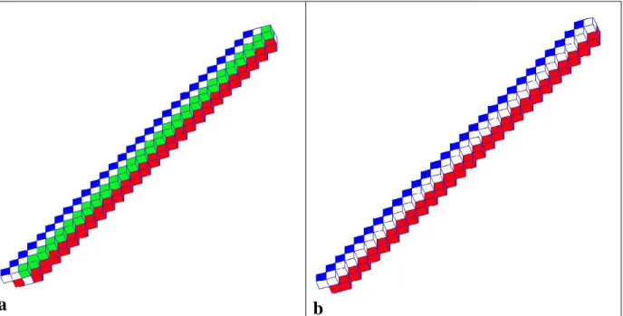
Fig. 2. Examples of step-shaped sets of meshes discretizing a fracture. a: steps that do not respect 199
the optimal contact between stairs; b: steps with optimal contact (only two rows of cells in 200
contact) between stairs. 201
202
The portion of fracture in Figure 2a is comprised of two steps and the connection between these 203
steps is assured by four lines of cubic elements. The green cubes of the top step are located at the 204
top of cubes which are not the border cubes of the bottom step. These green cubes of the top step 205
have to be suppressed while the white ones of the bottom step are preserved. Finally, the correct 206
fracture representation is given in Figure 2b and, by duplicating this elimination procedure over 207
all steps, the fracture is represented with the minimum number of elements connected by their 208
facets. The procedure is applied for each fracture of the network and the fracture intersections are 209
simply obtained as the resulting intersections of the fracture geometries. 210
211
In addition, within each fracture meshing, groups of cells have to be identified in view of the 212
equivalent approach presented below: the cells constituting the fractures are separated in two 213
distinct subsets. The first set, noted S set for "simple set", is that enclosing cells whose 214
neighbouring cells are all in the same plane. The second set, noted C (C stands for complex), 215
regroups two lines of N cells (denoted A and B in Figure 3). The property of a C set is to connect 216
two groups of S sets (i.e., C is the vertical part of a stair connecting two horizontal steps). For 217
both sets S and C, there are no fluxes through the top and bottom facets of cells. Two angles, θ 218
and β, are used to define the fracture plane orientation. θ (respectively, β) is the angle between 219
9
the horizontal plane x-y and the fracture intersection (trace) on the vertical plane x-z (respectively, 220
y-z). It must be noted that the configuration presented in Figure 3 occurs for 45°≥β >θ ≥0°. In 221
the sequel, this configuration will be studied as the example of reference and the procedure 222
dealing with other orientations will be then derived. 223 0000000000000 0000000000000 0000000000000 0000000000000 0000000000000 0000000000000 1111111111111 1111111111111 1111111111111 1111111111111 1111111111111 1111111111111 Q = 0 Q = 0X X 1 2 x y z β θ <−− fracture
a
00000000 00000000 00000000 11111111 11111111 111111110000000000000000000000000000 00000000000000 00000000000000 00000000000000 11111111111111 11111111111111 11111111111111 11111111111111 111111111111110000000000000011111111111111 00000000000000000000 00000000000000000000 00000000000000000000 00000000000000000000 00000000000000000000 00000000000000000000 00000000000000000000 00000000000000000000 00000000000000000000 00000000000000000000 00000000000000000000 00000000000000000000 00000000000000000000 00000000000000000000 00000000000000000000 00000000000000000000 00000000000000000000 00000000000000000000 00000000000000000000 00000000000000000000 00000000000000000000 00000000000000000000 11111111111111111111 11111111111111111111 11111111111111111111 11111111111111111111 11111111111111111111 11111111111111111111 11111111111111111111 11111111111111111111 11111111111111111111 11111111111111111111 11111111111111111111 11111111111111111111 11111111111111111111 11111111111111111111 11111111111111111111 11111111111111111111 11111111111111111111 11111111111111111111 11111111111111111111 11111111111111111111 11111111111111111111 11111111111111111111 0000000000000000000 0000000000000000000 0000000000000000000 0000000000000000000 0000000000000000000 0000000000000000000 0000000000000000000 0000000000000000000 0000000000000000000 0000000000000000000 0000000000000000000 0000000000000000000 0000000000000000000 0000000000000000000 0000000000000000000 0000000000000000000 0000000000000000000 0000000000000000000 0000000000000000000 0000000000000000000 0000000000000000000 1111111111111111111 1111111111111111111 1111111111111111111 1111111111111111111 1111111111111111111 1111111111111111111 1111111111111111111 1111111111111111111 1111111111111111111 1111111111111111111 1111111111111111111 1111111111111111111 1111111111111111111 1111111111111111111 1111111111111111111 1111111111111111111 1111111111111111111 1111111111111111111 1111111111111111111 1111111111111111111 1111111111111111111 00000 00000 00000 00000 00000 11111 11111 11111 11111 11111 Q = 04 β Q = 0Bi2 Q = 0Ai1 θ <−− column F <−− column L <−−−−−−−−−−−−−−−−−−−> N = 6 <−− line B Q = 0 6 <−− line A A fracture−−−> B Y Z X . F Lb
Fig. 3. Distinguishing between S and C set of cells according to the fracture location in the cells. 224
a: Simple (S) set encloses neighbouring cells all in the same horizontal plane; b: Complex (C) set 225
regrouping two lines of cells connecting two S sets. 226
3 Equivalent hydraulic conductivity computation
227
The approach for the computation of equivalent hydraulic conductivities is provided for the case 228
of a single fracture. Section 3.1 presents the basic idea supporting the method as well as basic 229
equations. The properties of the MHFE scheme essential for the approach are presented in 230
Section 3.2. In Section 3.3, the equivalent properties are derived for 45° ≥ > ≥ °β θ 0 and 231
extended to all geometries. 232
3-1 Introduction - a single fracture
233
As stated previously, the meshing of a fracture network is built using a regular grid. The 234
geometry associated with a single fracture appears as a stair-shaped set of parallelepiped elements 235
(see Figure 1 and Langevin, 2003; Hirano et al., 2010). 236
When modelling flow, the main concern is to evaluate the fluid flux occurring within the 237
geometrical representation of the fracture and compare it with a "reference", the latter being 238
10
analytical or stemming from a calculation over a very refined grid. For the problem of up-scaling 239
hydraulic conductivity in a discretized fracture network as that discussed above, the question of 240
fluid flux has to be handled at the scale of each grid cell. In the literature, a scalar value of 241
hydraulic conductivity per grid cell is often used (Svensson, 2001a; Hirano et al. 2010). This 242
choice may guarantee the flux conservation in 2-D cases (Fourno et al., 2007). Concerning 3-D 243
problems, this section will show why the use of a scalar value can be a flawed assumption and 244
how to upscale fracture hydraulic conductivity to correctly model the flux of a single fracture 245
intersecting a single rectangular cuboid (see Figure 4, with L , X L , Y L [L] the edge lengths of Z 246 the cuboid). 247 248 000000000000 000000000000 000000000000 000000000000 000000000000 111111111111 111111111111 111111111111 111111111111 111111111111 x y z β θ <−− fracture
a
0000000000000 0000000000000 0000000000000 0000000000000 0000000000000 0000000000000 1111111111111 1111111111111 1111111111111 1111111111111 1111111111111 1111111111111 x y zK
_
_
Ly Lxb
Fig. 4. A cell enclosing a portion of fracture (4a) and the equivalent hydraulic conductivity tensor 249
associated with that cell (4b). 250
251
The fracture is modelled as a porous medium with a hydraulic conductivity, k [LT-1] and an 252
aperture a [L]. The fracture orientation is characterized by the angles θ and β. The fracture is 253
not supposed to cross the top and bottom facets. The equations governing steady-state flow are 254
classically the Darcy's equation (Eq. 1) and the mass balance equation (Eq. 2): 255 . q= − ∇k h r r (1) 256 .q s ∇ =r r (2) 257
in which qr [LT-1] is the Darcy velocity, h [L] the head, s a source term [T-1]. 258
Considering the fracture position and orientation (Figure 4a), the boundary conditions of the 259
rectangular cuboid intercepted by the fracture are of no flow type at the top and the bottom facets. 260
Using a tensor notation, the classical analytical expression for the fluid flux, Q, is written as: 261
11 h L L L L c ka Q X X Y Y n ∇ = r 0 0 0 0 cos cos . sin . sin 0 . sin . sin cos cos θ β θ β θ β β θ (3) 262 with 2 1 2 2 ) sin sin 1 ( − β θ = n c . 263
For no flow boundary conditions at the top and bottom facets of the intersected parallelepiped 264
element, the equivalent hydraulic conductivity tensor, K , can be calculated as: 265 = 0 0 0 0 cos cos sin . sin 0 sin . sin cos cos θ β θ β θ β β θ z nL c ka K (4) 266
Equation 4 demonstrates that the equivalent hydraulic conductivity has to be a tensor to correctly 267
model the fracture flux magnitude and direction. Notably, when the opposite grid cell facets are 268
not identical (as for unstructured meshing using the corner point grid technique) the hydraulic 269
conductivity tensor is not symmetric. 270
271
In this paper, we propose to model fractures (and by extension fracture networks) using 272
simplified diagonal hydraulic conductivity tensors. Considering that the off-diagonal elements of 273
the tensor (Equation 4) depend on the product sinβsinθ, the simplification into a diagonal 274
tensor will be valid for values of β and/or θ close to zero. This geometrical configuration 275
corresponds to sub-horizontal and sub-vertical fault networks. Equation 4 is obtained for specific 276
flow boundary conditions of no-flow at the top and bottom facets; which contradicts the above 277
statement of inferring diagonal tensors for sub-vertical fractures. Expressions similar to (4) can 278
be obtained by permutations between directions x, y, and z so that to deal with sub-vertical 279
fractures and flowing boundary conditions on the top and bottom facets (see Table 1 at the end of 280
Section 3). At this stage of the paper, we focus the analysis on fractures honouring the condition 281 ° ≥ > ≥ ° 0
45 β θ and decomposed into S or C subsets of cells (see Section 2). The equivalent 282
12
permeability tensor is computed analytically thanks to MHFE properties (Section 3.2) for S and C 283
groups of cells (Section 3.3). 284
3-2 Flow governing equation and MHFE scheme
285
The purpose of the present section is to provide the reader with some basic knowledge about the 286
MHFE scheme. In particular, through the introduction of additional unknowns termed head 287
traces, the water mass conservation principle can be formally established at the scale of a single 288
cell or of a group of cells. This property is fundamental for the FCVA presented here and leads to 289
the equivalent properties derived in the next Section. As previously introduced, our approach is 290
based on diagonal hydraulic conductivity tensors. The steady-state flow equations (1) and (2) are 291
rewritten in the form: 292 h K q set ∇ − = r r (5) 293 s q= ∇r.r (6) 294 with set
K the diagonal hydraulic conductivity tensor [LT-1]. In the following, the index "set" will 295
be replaced by S or C according to the S or C set of cells considered. 296
297
The goal is to relate equivalent hydraulic conductivity tensor components ( set x
K ,Kyset, set z
K ) to the 298
fracture hydraulic conductivity, k. The numerical scheme used relies on mixed finite elements 299
that preserve by construction the fluid fluxes normal to the interfaces between adjacent elements. 300
To this end, specific variables are manipulated including the mean head h over an element E E 301
and the mean heads (also called traces) E i
Th over the facet i of the element E. In the end, the 302
elementary scheme involves 13 unknowns for a cubic element, i.e., 6 fluxes Q , 6 head traces i Th i
303
and the mean head E
h . Flow is calculated by handling the head traces as principal variables with 304
the following form for fluxes and mean head (Mose et al., 1994; Dabbene et al., 1998; Bernard-305 Michel et al., 2004): 306 307 6 .. 1 ) .( ) ( ) ( 1 − 1 1 = =
∑
−∑
− − i with Th M M h Q j E j E ij j E ij E E i (7) 30813
∑
∑
= i E i i i E i E Th h α α (8) 309 with =∑
− j E ij E i (M ) 1 α , =∫
− E j set t i E ij w K w dEM (r ) ( ) 1(r ) ,M−1the inverse matrix of M and wi
r 310 defined as
∫
= j F wi ndFj δij r r. . Considering cubic elements (∆3
) and diagonal hydraulic 311
conductivity tensors,
set
K , the hybrid mass matrix E
M writes: 312 313 2 1 0 0 0 0 1 2 0 0 0 0 2 1 0 0 0 0 1 2 1 6 0 0 0 0 1 2 0 0 0 0 1 2 0 0 0 0 set set z z set set z z set set y y E set set x x set set y y set set x x K K K K K K M K K K K K K − − − = − ∆ − − (9) 314 315
Equation (7) can be easily written as 316
K h
Q=B T (10)
317
in which B depends on values of fracture hydraulic conductivity. K
318 319
Thanks to Equation (10), it is possible to associate numerical fluxes for a cubic discretization to 320
an analytical flux whatever the head gradient. This means we are able to propose equivalent 321
hydraulic conductivity tensors for S and C set of cells to obtain the exact flow occurring in a 322
fracture. 323
14
3-3 Expression of fluxes with MHFE and derivation of equivalent hydraulic conductivities
324
By accounting for both the geometry of the modelled fractures and the MHFE numerical 325
formalism, an analytical expression of the fluxes in each cell as a function of head gradients is 326
obtained. Mass balance, head, head gradient and velocity are estimated within the element on the 327
basis of the traces of heads along the facets of the element. Given the geometrical considerations 328
reported in Figure 2, each element of the grid has a limited connectivity with its neighbours. This 329
point is used to obtain the analytical expression of the MHFE fluxes. As mentioned earlier, the 330
equivalent properties are computed for two types of cell groups for which no flow occurs through 331
their top and bottom facets. 332
3-3-1 The S set of cells 333
In the case of cells from the S set (see Figures 3a and 4b), equations of MHFE fluxes are easy to 334
obtain. With reference to facet notations reported in Figure 5, it can be noted that along the x 335
direction, the unknown is QxS =Q4S = −Q6S. By using Equation (10), it comes: 336 x S x S x K h Q =− .∆.∆ with ∆ =hx Th4−Th6 (11) 337
Along the y direction, QSy =Q5S =−Q3S can be written as: 338 y S y S y K h Q =− .∆.∆ with ∆ =hy Th3−Th5 (12) 339
For the set S of cells, the following equivalent hydraulic conductivity tensor (
S
K ) is obtained by 340
flux conservation (see relations 3, 11 and 12): 341 cos 0 0 cos 0 0 cos 0 0 cos S S x x S n S y S S y z n a K k K c K K with a K k K c θ = ∆ β = β = ∆ θ (13) 342
Notably, K is not defined and can be set up at any value, for instance that of zS K yS
343
3-3-2 The C set of cells 344
The case of cells from the C set is trickier (Figures 3b and 5b). We denote by A and B the top and 345
bottom lines of cells, respectively; the element Ai (respectively Bi) is the ith element of line A 346
(respectively, line B) and QjAi is the flux through the facet j of the cell Ai (see Figure 5a for facet 347
numbering). 348
15 349 x y z Facet 2 Facet 4 Facet 6 Facet 3 Facet 5 Facet 1 .
a
00000000 00000000 11111111 11111111 00000000 00000000 00000000 11111111 11111111 11111111 00000000000000000000 00000000000000000000 00000000000000000000 00000000000000000000 00000000000000000000 00000000000000000000 00000000000000000000 00000000000000000000 00000000000000000000 00000000000000000000 00000000000000000000 00000000000000000000 00000000000000000000 00000000000000000000 00000000000000000000 00000000000000000000 00000000000000000000 00000000000000000000 00000000000000000000 00000000000000000000 00000000000000000000 11111111111111111111 11111111111111111111 11111111111111111111 11111111111111111111 11111111111111111111 11111111111111111111 11111111111111111111 11111111111111111111 11111111111111111111 11111111111111111111 11111111111111111111 11111111111111111111 11111111111111111111 11111111111111111111 11111111111111111111 11111111111111111111 11111111111111111111 11111111111111111111 11111111111111111111 11111111111111111111 11111111111111111111 00000000000000000000 00000000000000000000 00000000000000000000 00000000000000000000 00000000000000000000 00000000000000000000 00000000000000000000 00000000000000000000 00000000000000000000 00000000000000000000 00000000000000000000 00000000000000000000 00000000000000000000 00000000000000000000 00000000000000000000 00000000000000000000 00000000000000000000 00000000000000000000 00000000000000000000 00000000000000000000 00000000000000000000 11111111111111111111 11111111111111111111 11111111111111111111 11111111111111111111 11111111111111111111 11111111111111111111 11111111111111111111 11111111111111111111 11111111111111111111 11111111111111111111 11111111111111111111 11111111111111111111 11111111111111111111 11111111111111111111 11111111111111111111 11111111111111111111 11111111111111111111 11111111111111111111 11111111111111111111 11111111111111111111 11111111111111111111 00000 00000 00000 00000 00000 11111 11111 11111 11111 11111 Q = 0B4 Q = 0A 6 β θ −−> Column F −−> Column L z y xFacet 4 of the L column
|_ L6 _|
|_ L4 _|
Fracture
Facet 6 of the F column
F L
b
0000000 0000000 0000000 1111111 1111111 1111111 x z y <−− line B <−− line A Q = 0 Q = 0A2 B 1 CFig. 5. a: facets numbering of a cubic mesh for flux calculations; b: fracture location in a set of 350
2N cells belonging to a complex (C) set of cells; c: two cells of a C set of cells (see Fig. 5b) with 351
their local boundary conditions. 352
353
The following properties characterize the elements of the set C: 354 • Boundary conditions : 355 0 1 2 6 4 0 0... 0 i i N A B A B Q Q i N Q Q = = = = = (14) 356 • Continuity conditions: 357 1 1 6 4 6 4 i i i i A A B B Q Q Q Q + + = = (15) 358 • Geometrical conditions 359
16
N, the number of cells in a line of a C set, may be evaluated as a function of θ and β from the 360
fracture position inside the C set (Figure 5b). We consider the intersections (traces) of the 361
fracture with facet 4 of the first column of cells and facet 6 of the last (Nth) column of cells. We 362
also assume that the two traces of fracture touch the horizontal plane separating the two lines of C 363
cells, at the edge between facet 4 – facet 5 for the first column and the edge between facet 6 – 364
facet 3 for the last column (see Figure 5). By denoting dz the variation of elevation of the traces 365
on facets 4 and 6 mentioned above we note 366 tan tan , tan tan dz dz N N β β θ θ = = ⇒ = ∆ ∆ (16) 367
It is obvious that the evaluation of N is an approximation because all the triplets
(
θ β, ,∆)
do not 368allow an exact positioning of the fracture traces as assumed above. Usually, one may miss or add 369
one cell compared with the real number of cells in a C set. Another observation is helpful. 370
Considering the facet 6 of the first column (column F in Figure 5b) and the facet 4 of the last one 371
(column L in Figure 5b), one can notice that the length L6 and L4 are equal yielding 372 0 0 4 6 ; 4 6 N N A B B A Q = −Q Q = −Q (17) 373 374
The final relation deduced from geometrical observations is that describing how the flux crosses 375
the last column (and by symmetry the first column too). Considering the facet 4 of the last 376
column and the line A, the height variation of the fracture trace equals dz= ∆tanθ . On this facet 377
(facet 4, line A) the length of the fracture trace equals 4 sin
A dz
L
β
= while the total length on the 378
facet 4 (line A plus line B) is
β cos ∆ = L . Knowing that 4 4 N A C A x Q =Q L L , we obtain: 379 4 tan . tan N A C x Q = θ Q β (18) 380 A scalar value β θ tan tan =
U is introduced to simplify the previous relation C x A Q U Q N . 4 = . 381 382
17
With the above conditions, we try now to express the flux in C set cells along the x and y 383
directions C x
Q , C y
Q as functions of ∆, θ and β. Two directions of head gradients are applied
384
onto the former systems to derive the associated flux along the same directions. 385
- MHFE flux along the x direction 386
Knowing that the hydraulic conductivity tensor of each element is diagonal, the following 387
conditions can be expressed: 388 0 3 3 5 5 4 6 0 0... 0 0... i i i i N A B A B A B C x Q Q i N Q Q i N Q Q Q = = = = = = = − = (19) 389
with Q the flux of C set along the x direction. Using the boundary, flow and geometrical Cx
390
conditions and Equation (10), the flow C x
Q can be finally expressed as: 391 2 2 4 1 3 3 C C C x z x x C C z x K K Q h U U N K K ∆ = − ∆ + − + (20) 392 393
Using the N and U values previously determined the final expression is obtained: 394 395 2 tan tan 2 4 tan tan tan 1 tan 3 3 C C C x z x x C C z x K K Q h K K ∆ = − ∆ θ θ β β β + − + θ (21) 396
- MHFE flux along the y direction 397
In the whole set C of cells, all the columns play the same role which allows simplifying the 398
identification of fluxes along the y direction to the flux along a single column (Figure 5c). We 399
note Q~Cy the flux of a C set column along the y direction.
400
The flow boundary conditions are: 401 4 4 0 ; 6 6 0 ; 5 3 A B A B B A C y Q =Q = Q =Q = Q = −Q =Q% (22) 402 C y
Q~ is easily obtained by solving the following equations: 403
18 5 3 2 1 3 5 4 6 2 0 3 2 0 0 B A C y C C B A y z C y C C y B A y z B A Q Q Q K K Q Q Q h K K Q Q Q Q − = − = ⇒ = − ∆ ∆ + − = − = % (23) 404
For N columns of cells with N =tanβ tanθ , the total flux C y
Q along the y direction writes 405 obviously: 406 C y C y Q Q .~ tan tan θ β = (24) 407
- Derivation of equivalent hydraulic conductivities 408
Considering the relations, 3, 21, 23 and 24, the equivalent hydraulic conductivity tensor of C set 409
cells can be written as: 410 cos 2 2 4 cos 0 0 1 3 3 0 0 0 0 3 cos 2 cos C C x z C C C n x C z x C y C C C y z z C C y z n K K a k N c K N U K UK K K with K K K a N k K K c θ = ∆ β + − + = β = + ∆ θ (25) 411
With the assumption yC C
z K
K = , the following expressions are obtained: 412 2 2 2 tan 2 tan 1 tan 3 tan cos cos sin 2 sin 4 cos 3 cos C x n C y n a K k c a K k c θ θ + − β β θ = ∆ β θ − β β = ∆ θ (26) 413
It is interesting to note that: 414
the hydraulic conductivity tensor is established for 45°≥β >θ ≥0° (Figures 5a, 5b), 415
for the case β =θ =0 , there are obviously only cells of S type and the classical 416 correction ∆ a is obtained, 417 for β =θ , by symmetry C y C x S y S x K and K K K = = . 418 419
19
The equivalent tensors can also be obtained for other fracture orientations by means of geometrical permutation
420
between the x, y and z directions so that the former results are extended to all configurations. Considering the vector
421
normal to the fracture plane, it is possible to switch the values of the equivalent tensor (by also changing the basis
422
vector) and determine the values of θ and β with 45°≥β >θ ≥0°. The results are summed up in Table 1 in
423
terms of equivalent tensor set
K .
424
Configuration resulting tensor configuration case
1 θ β
=
set z set y set x setK
K
K
K
0
0
0
0
0
0
nmax =nz & nmin =ny) arctan( ) arctan( z y z x n n n n = = ⇒ θ β 2 θ β
=
set z set x set y setK
K
K
K
0
0
0
0
0
0
nmax =nz & nmin =nx) arctan( ) arctan( z x z y n n n n = = ⇒ θ β 3 β θ . .
=
set y set z set x setK
K
K
K
0
0
0
0
0
0
nmax =ny & nmin =nz) arctan( ) arctan( y z y x n n n n = = ⇒ θ β 4 β θ
=
set x set z set y setK
K
K
K
0
0
0
0
0
0
nmax =ny & nmin =nx) arctan( ) arctan( y x y z n n n n = = ⇒ θ β 5 β θ = set y set x set z set K K K K 0 0 0 0 0
0 nmax =nx & nmin =nz
) arctan( ) arctan( x z x y n n n n = = ⇒ θ β 6 β θ
=
set x set y set z setK
K
K
K
0
0
0
0
0
0
nmax =nx & nmin =ny) arctan( ) arctan( x y x z n n n n = = ⇒ θ β
Table 1. How to correctly orientate the equivalent tensor according to the fracture orientation. θ (respectively, β) is
425
the angle between the horizontal plane x-y and the fracture intersection (trace) on the vertical plane x-z (respectively,
426
y-z)
20
4 Evaluation of equivalent properties
428
T
he FCVA is now tested against analytical results for flow: 1- in a single fracture with various 429dips and strikes, and 2- in regular fracture networks. As already mentioned, the equivalent (full) 430
tensor is diagonal. The approximation is strictly valid for sub-vertical or sub-horizontal fractures. 431
The non-diagonal components increase as a function of sinβsinθ. For all configurations, the 432
hydraulic conductivity of the fracture(s) is 3.8×10⁻⁸ m.s-1 (= 4 darcys), the fracture aperture is 433
2.10-2 m. In Section 4.2, the case of fracture networks is considered with emphasis on the specific 434
issue of fracture intersections. 435
4-1 Sensitivity to the orientation for flow in a single fracture
436
The fracture crosses the regular grid from one side to the opposite side. Different dip and strike 437
configurations are tested. For each mesh direction, i = x, y, z, the breakthrough flux, Qnumi is
438
calculated using the MHFE voxel approach. An analytical expression of this flux i ana
Q is also 439
obtained considering Equation (3) and for whichL , X L , Y L are now the medium lengths. For Z 440
each fracture orientation, both analytical and numerical up-scaled hydraulic conductivity tensors 441
are derived from fluxes. The diagonalized "numerical" tensor upsnum n
K , resulting from the FCVA 442
is compared with the analytical one upsana n
K ,
and a relative error is defined as the ratio 443 ana ups n ana ups n num ups n K K K , , , −
with the index n referring to the minimal, intermediate and maximal value of 444
the tensor components. Table 2 summarizes the results for the different fracture orientations. 445 446 447 448 449 450 451 452 453
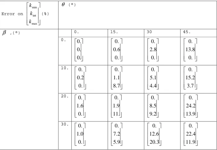
21 Error on max int min k k k (%) θ (°) β ,(°) 0. 15. 30 45. 0. . 0 . 0 . 0 . 0 6 . 0 . 0 . 0 8 . 2 . 0 . 0 8 . 13 . 0 10. . 0 2 . 0 . 0 7 . 8 1 . 1 . 0 4 . 4 1 . 5 . 0 7 . 3 2 . 15 . 0 20. . 0 6 . 1 . 0 . 11 9 . 1 . 0 2 . 9 5 . 8 . 0 9 . 13 2 . 24 . 0 30. . 0 0 . 1 . 0 9 . 5 2 . 7 . 0 3 . 20 6 . 12 . 0 9 . 11 4 . 22 . 0
Table 2. Errors on equivalent tensor of hydraulic conductivity between FCVA and analytical 454
values for the cases of a single fracture with different orientations. θ (respectively, β) is the angle 455
between the horizontal plane x-y and the fracture intersection (trace) on the vertical plane x-z 456
(respectively, y-z) 457
458
Four points can be extracted from Table 2. 459
1. For θ =0 and β =0, the local hydraulic conductivity of the fracture is simply corrected 460
by the ratio
∆
a
and exact fluxes are obtained by construction (i.e., null error in Table 2). 461
2. Equation 4 shows that for the values (θ =0 and β ≠0) or (θ ≠0 and β =0) the 462
analytical hydraulic conductivity tensor is diagonal as is also the case for the numerical 463
tensors of the S and C cell sets of the FCVA. The consequence is that for configurations 464
in which one of the angles θ or β is null, the flux directions are perfectly modelled and 465
errors are of only a few percent. 466
3. For other fracture orientations, precision depends on the value of sinβsinθ (see Eq (3)). 467
When considering diagonal hydraulic conductivity tensor in the voxel approach, the non-468
22
diagonal flux values (Eq (2)) are supposed to be negligible. This is not always the case 469
and the larger the value of sinβsinθ, the larger the errors become. 470
471
This test case confirms that the equivalent properties are exact for fractures aligned with a main 472
grid direction. The error increases when fracture orientations deviate from such conditions. The 473
maximum error is less than 30%. For a real case study, when feasible, a main axis as close as 474
possible to the fracture plane orientations should be chosen. 475
476
4-2 Hydraulic conductivity of regular fracture networks
477
The second case study is that of a regular fracture network in a block of 100×100×8 m3. The 478
system is not strictly three-dimensional because fractures are vertical and main hydraulic 479
gradients in the block concealing the fracture network are horizontal. These settings, however, 480
allow a better assessment of the influence of fracture intersections. We first show that some 481
constraints in terms of grid size exist to actually represent the connectivity of the fracture network 482
on a regular grid. The smaller the grid size, the closer the representation is to the geometrical 483
reality. The contact surface between two intersecting fractures obviously depends on the size of 484
the mesh, so that head gradients as well as flux exchanged across the intersection should 485
intuitively depend upon the grid size. The convergence of the flux in the network toward a 486
constant value with grid size is reached for cell dimensions tending to the fracture aperture. 487
488
The fracture network (Figure 6) is made of four families of vertical fractures with directions of 489
10°, 34.5°, 100°, and 124.5° (Figure 7). The network is mapped onto five regular grids with 490
meshes varying from 0.1 m on a side up to 4 m (Figures 6a, 6c). For the purpose of comparison, 491
the network is also explicitly meshed (without mapping). No special effort to optimize the 492
number of cells was done for this explicit meshing and both fracture planes and fracture 493
intersections are discretized at a mean cell size of 0.2 m (Figure 6b). With the network topology 494
and the explicit meshing, the modelling exercise is very similar to that depicted in Karimi-Fard et 495
al. (2006). This exercise will also serve as reference for evaluating accuracy of fluxes draw from 496
the FCVA approach. The properties associated with the fractures of all families are constant: 497
hydraulic conductivity (3.8×10⁻⁸ m.s-1) and aperture (2.10-2 m). Figure 6 shows the same fracture 498
23
network mapped onto two regular grids, the first with a fine space step (0.2 m, Figure 6a), the 499
second with a coarse step (4 m, Figure 6c). In the second case, the connectivity of the system is 500
not represented. The contact surface at the fracture intersections is better modelled for the finest 501
grid. The validation of the FCVA is addressed by considering numerical fluxes from FCVA, 502
analytical fluxes from (3) and numerical fluxes from the explicit meshing of the fracture network. 503
We note Qi j the flux through the facet j (or equivalently along direction j) considering a head
504
gradient along the direction i. The specific label Qi jexpl denotes fluxes from the explicit meshing of 505
the network. Using Equation 3, analytical fluxes of the whole network ana i j
Q are calculated as the 506
sum of analytical fluxes associated with the individual fractures. 507
a
b
c
Fig. 6. Discretization of a regular fracture network by using a fine grid size of 0.2 m on a side (a) 508
and a coarse grid size of 4 m (c). In b a portion of the explicit meshing of the fracture network for 509
the purpose of comparison with the mapping procedure. 510
First family set Qx Qy Qz
0 1 2 3 4 5 6 Num, grad(h)=x Ana, grad(h)=x Num, grad(h)=y Ana, grad(h)=y Num, grad(h)=z Ana, grad(h)=z
24
Second family set Qx Qy Qz
-1 -0,5 0 0,5 1 1,5 2 2,5 3
Third family set Qx Qy Qz
0 0,5 1 1,5 2 2,5 3 3,5 4 4,5 5
Fourth family set Qx Qy Qz
-1 -0,5 0 0,5 1 1,5 2 2,5
Fig. 7. Calculations of fluxes in a block enclosing different families of parallel fractures. Qx, Qy, 511
and Qz refer to the fluxes in the whole block along the x, y and z directions, respectively. Labels 512
"Ana" and "Num" refer to analytical solutions and numerical ones. The fluxes Qx, Qy and Qz are 513
calculated for three main head gradients along the x, y and z directions. 514
In a first stage, we study the fluxes in each of the four fracture families of the fracture network 515
independently (Figure 7). This is done in order to compare FCVA numerical flux values with 516
analytical ones. The error should be stronger than for the single fracture test case because there is 517
a side effect for the fractures which cross the fractured block from a vertical facet to a vertical 518
adjacent one. Indeed, for these fractures, the no-flow boundary condition is not respected for the 519
S and C sets of cells that touch the sides of the block. The fluxes through each facet of the 520
fractured block are reported in Figure 7 considering three head gradient directions. As expected, 521
25
the flow is correctly modelled for each fracture set. The order of magnitude of the different fluxes 522
is well captured, with relative errors between analytical and numerical fluxes less than 10%. 523
524
In a second stage, we model flow into the whole network including the four fracture families. 525
This exercise is performed by assigning the fracture intersection with the highest hydraulic 526
conductivity value of the fractures present at the intersection. The analytical fluxes are still 527
obtained as the sum of fluxes in each fracture (drawn from Equation 3). The above settings 528
correspond to the classical approach of Oda (1986) which, in terms of fracture intersections, is 529
equivalent to assume independent flow between fractures. If the same strategy is applied to 530
numerical fluxes (i.e., by summing the numerical fluxes of each fracture family), it is obvious 531
that the total numerical fluxes will be similar to analytical ones simply because FCVA is accurate 532
for poorly connected fracture networks. On the other hand, calculating flux over the whole 533
network, including interactions between fractures at their intersections, will cause the numerical 534
fluxes to diverge from analytical ones. First, we note that the numerical fluxes calculated from a 535
network explicitly meshed at small mesh size (see above) are similar to that from the analytical 536
ones. This is the consequence of the explicit and precise meshing of fracture intersections to 537
which the highest local hydraulic conductivities are assigned. In addition there is no dead-ends in 538
the fracture network. No forces (except the local conductivity) are opposed to flow in each 539
fracture with the consequence that the total flux in the block is the mere addition of each fracture 540
contribution. In the end, the differences between FCVA and analytical (or explicit meshing) 541
approaches must be associated with the FCVA geometrical representation of the fracture network 542
and depend on the discretization. Figures 8 and 9 report on analytical fluxes, numerical fluxes 543
from an explicit meshing of the network and FCVA fluxes values of the fractured block for 544
different mesh size values (from 0.1 to 4 m). 545
26 -0,5 1,5 3,5 5,5 7,5 9,5 11,5 13,5 15,5 17,5 0 0,5 1 1,5 2 2,5 3 3,5 4
Qxx (x 1.e-8) Qxx_ana ≈ Qxx_expl (x 1.e-8)
Qyy (x 1.e-8) Qyy_ana ≈ Qyy_expl (x 1.e-8)
Qxy (x 1.e-8) Qxy_ana ≈ Qyx_ana ≈ Qxy_expl ≈ Qyx_expl (x 1.e-8)
Qyx (x 1.e-8) Qzz_ana ≈ Qzz_expl (x 1.e-7)
Qzz (x 1.e-7) 547
Fig. 8. Evolution of calculated fluxes in a fractured block (network in Fig. 6) with elementary 548
mesh sizes evolving from 0.1 to 4 m on a side. The notation Qij (i, j = x, y, z) refers to fluxes 549
along the j direction for a main head gradient along the i direction. The analytical values "Ana" 550
are that from the Oda's assumption stating independent flow between fractures. The values 551
labelled "Expl" stem from calculation over a fracture network explicitly (completely) meshed for 552
both fracture planes and fracture intersections. 553 554 0 20 40 60 80 100 120 140 0 0,5 1 1,5 2 2,5 3 3,5 4 ∆ %
% Qxx % Qyy % Qzz % Qxy % Qyx
555
Fig. 9. Fluxes through a fractured block (network in Fig. 6). Evolution of the relative error (Qnum 556
– Qana)/Qana with elementary mesh sizes in the range 0.1 – 4 m. Qij (i, j = x, y, z) refers to fluxes 557
along the j direction for a main head gradient along the i direction. 558
27
The main observation is a convergence of FCVA numerical fluxes values toward analytical ones 559
when decreasing the mesh size. For finer grids (mesh size values of 0.1 – 1 m), the relative error 560
on fluxes is close to 10 %, which is generally very reasonable in view of the weak precision on 561
hydraulic property measurements in natural media. When increasing the mesh size, the evolution 562
of relative errors on fluxes is not monotonic (Figure 9), especially for marginal fluxes Qij, i.e., 563
fluxes along direction i when applying a main head gradient along direction j, j≠i. Relative errors 564
may reach 50-100% on Qij j≠i but theses fluxes are also ten times less than fluxes Qii making 565
therefore a relative error of 50% on Qij, something small compared to the total flux conveyed by
566
the fractures. The non-monotonic behaviour of errors comes from the competition between: 1- 567
the calculation of the number N of cells in a ''Complex'' C set (cells connecting by their horizontal 568
facets two portions of planes of different elevation); 2- some cells at the limits of the fractured 569
block may show non-null fluxes through their top and bottom facets, which contradicts the 570
assumption used to calculate hydraulic conductivity tensors (see Section 3). As expected 571
however, for coarse discretizations with rough representations of fracture intersections, the 572
general trend is that of errors on equivalent conductivity tensors increasing quickly with the 573
discretization size. The first criterion for providing accurate results is to respect the connectivity 574
of the fracture network; as a rule of thumb, the smallest matrix block between fractures should be 575
represented by a few cells. However, by considering the order of magnitude of errors with 576
reference to computation efforts, simulations based on coarse discretizations may be very 577
attractive for preliminary results. These computations efforts are summed up in Table 3 for 578
different FCVA discretizations. 579
580 581
∆ (m) Number of cells Meshing CPU time (s) Flow (3directions) CPU time (s) 4 884 3 1 2 4108 7 6 1 18240 24 34 0.4 121440 193 370 0.2 495120 864 23257
Table 3. Computation times for meshing and calculating fluxes over a fracture network (network 582
in Fig. 6) at different cell sizes. 583
584 585
28
In a final exercise, flow simulations are performed for different assumptions regarding the 586
behaviour of fracture intersections. The goal is not to propose a third validation exercise of the 587
FCVA but to illustrate how an additional freedom degree can be added in modelling flow by 588
introducing different hydraulic behaviours at fracture intersections. Ideally, the choice of 589
intersection modelling should be dictated by geological considerations. In practice, the values of 590
hydraulic conductivity at fracture intersections could have some statistical dependence on the 591
values of intercepting fractures, or be in a range of values supposed to mimic a set of objects 592
between clogged and widely opened intersections. Four intersection models are considered in the 593
following sensitivity study. A first choice is to assign, at the intersection cells, the highest 594
hydraulic conductivity of intersecting fractures and correct it to obtain the equivalent 595
permeability tensor (Model I1, already used in the previous simulations). Another option (model 596
I2) is to sum each fracture contribution and to correct the obtained value. These choices do not 597
significantly change the order of magnitude of hydraulic conductivity values applied to the 598
intersection cells. Thus, to model extreme cases as clogged or opened intersections, we apply a 599
correction to the highest hydraulic conductivity value of fractures present at the intersection (i.e., 600
corrections to I1), respectively int 10−6
∆ = a
kcor for a clogged intersection (model I3a) or
∆ = a
kintcor 10 601
for an opened intersection (model I3b). 602
603
The influence of these models I1 to I3b is studied for the network of four fracture families 604
discussed above and discretized at the constant grid size of 0.4 m. The incidences in terms of 605
breakthrough fluxes through the facets of the fractured block are illustrated in Figure 10. 606