HAL Id: hal-00630711
https://hal.archives-ouvertes.fr/hal-00630711
Preprint submitted on 10 Oct 2011HAL is a multi-disciplinary open access archive for the deposit and dissemination of sci-entific research documents, whether they are pub-lished or not. The documents may come from teaching and research institutions in France or abroad, or from public or private research centers.
L’archive ouverte pluridisciplinaire HAL, est destinée au dépôt et à la diffusion de documents scientifiques de niveau recherche, publiés ou non, émanant des établissements d’enseignement et de recherche français ou étrangers, des laboratoires publics ou privés.
Price expectations and price dynamics: the case of the
rice sector in developing Asia
Thomas Barré
To cite this version:
Thomas Barré. Price expectations and price dynamics: the case of the rice sector in developing Asia. 2011. �hal-00630711�
E-mail address: thomas_barre@yahoo.fr
Price expectations and price dynamics: the case of the rice sector in
developing Asia
Thomas BARRÉ
ERUDITE – Université Paris – Est &
CES – Universté Paris 1 Panthéon Sorbonne
02/10/2011
Abstract: Uncertainty is a crucial issue for producers who must make input decisions without
knowing prices and without perfect knowledge of realized output. In this context, price expectations strongly determine the production choices and market prices that result from market-clearing conditions. This study analyzed the role that price expectations play in price dynamics, developing a theoretical model of trade in varieties following Armington (1969) and augmented with yield and price uncertainty to highlight several main determinants of domestic producer prices, including exchange rates, proximity to world markets, input prices, natural disasters, and producers’ expectations. An econometric estimation of the rice sector, using a panel of 13 developing Asian countries during 1965–2003, confirmed that expectations count, with a 1% increase in the expected price resulting in a 1.18% decrease in the market price. A simulation exercise based on these empirical results demonstrated that forecasting errors are large. Specifically, Asian rice farmers have a 50% chance of making prediction errors of 10% or more on the final market price. This high error rate suggests the need for developing ways of sharing information, such as radio programs dedicated to agricultural producers or the introduction of futures markets, to stabilize agricultural incomes.
2
The food crisis of 2007–2008 and the recent surge in food prices have renewed the interest of economists in employing policy tools or instruments appropriate for managing agricultural price volatility. As proposed by Galtier (2009), these policy tools can be classified into four categories based on their objective (price stabilization or reduction in the effect of price instability) and their ―mode of governance‖ (public or market based). The problem often pointed with price stabilization is that it can distort the informational content of prices. If the state intervenes to stabilize prices – either through public buffer stocks or trade restrictions – producers are incentivized to either overproduce when the state guarantees a floor price to producers or under produce when it sets a ceiling price for consumers. This policy, however, disrupts the negative correlation between prices and production levels and can cripple the government revenues, as was the case in 2007–2008. On the other hand, market-based instruments like futures hedging coupled with transfers to the most vulnerable populations unable to use market-based instruments appears to be the best way to protect the poor against price volatility without affecting prices. But the lack of acceptance of such instruments aimed at protecting peasants against price volatility by developing countries (CRMG 2008) has led researchers to focus on market based instruments that can stabilize prices without affecting their informational content. These policies are supposed to contribute towards a good match between supply and demand and stabilize prices thanks to improvements in spatial and temporal integration of markets by the development of transport networks, storage facilities and quality standards. Finally, the recent surge in food prices has demonstrated that while state intervention remains necessary to avoid domestic food crises and protect the most vulnerable populations, it can also induce hoarding behavior among consumers and speculators, putting additional pressure on prices (Timmer 2009), providing a new argument against state intervention.
3
As the usefulness of price management policies depends on the sources of price dynamics, the core issue in the debate on the use of the appropriate instruments to manage price volatility is to determine the forces behind the formation of prices. Galtier (2009) distinguishes three main forces that determine price changes: The first cause of agricultural price volatility is ―natural instability‖, which comes from natural hazards that affect production. When a natural disaster occurs, production decreases, resulting in excess demand with respect to supply and an increase in market prices. A second source of instability of domestic prices is imported, that is, it is caused by changes in parity prices and substitutions in consumption baskets by world customers. Trade policies and exchange rates are key factors in this form of instability. A third source of instability is the endogenous fluctuations generated by the instability of market players’ price expectations. In this case, ―domestic prices can be unstable without any movement in market fundamentals (domestic supply, demand curves, and terms of trade)‖. For example, farmers increase their production level if price expectations increase, which in turn generates a drop in prices because supply exceeds demand.
This article focuses on the role of price expectations and develops a model for agricultural commodities price formation based on an economic geography framework (following Armington 1969) augmented with price and yield uncertainty. The model was tested on an unbalanced panel dataset of producer prices for rice in 13 Asian countries. The theoretical model appears relevant as demonstrated by the estimation results. First, estimated structural parameters corresponded to those found in the literature and to prior knowledge, with an Armington elasticity close to 6 and returns to scale approximately equal to 0.9. Second, a simulation exercise determined that the quality of price expectations was so that farmers have a 50% chance of making a forecasting error being greater than 10% of the market price and showed that the model can reproduce some
4
of the main characteristics of price changes (volatility, skewness, and kurtosis). The analysis of the data also showed that price expectations were a crucial determinant of price formation. Given the extent of forecasting errors, improvements in the informational network should be at the top of the reform agenda. In particular, the development of futures markets in the rice sector, combined with investments in radio programs dedicated to farmers, could address the poor price expectations issue and help in price stabilization, which is an important condition for sustainable growth ( Ramey and Ramey 1995).
The paper is organized as follows: Section 1 briefly presents the literature on agricultural commodity price formation; Section 2 describes the theoretical model and estimation method; Section 3 presents the data and empirical estimation results; and Section 4 concludes.
Taxonomy of price dynamics explanations
As noted by Gouel (2011), most of the literature on agricultural price instability is characterized by a dichotomy between endogenous and exogenous explanations for price dynamics. In general, exogenous explanations identify harvest shocks as the cause of price fluctuations, and endogenous explanations identify errors in expectations as the cause. Other researchers have focused on monetary explanations for price changes (Frankel 1986) or the role of exchange rates and the terms of trade (Liefert and Persuad 2009).
The original model of endogenous fluctuations can be traced back to Ezekiel (1938) and his cobweb theorem, in which it was assumed that farmers formed their price expectation on the basis of the observed actual price, . According to this theorem, when the actual price is high, farmers anticipate future prices to be high and increase their production level. This
5
increase in the quantity harvested decreases the price. In the next period, given the low actual price, farmers anticipate a low future price and so will plan to produce less, which will in turn increase the price of the harvested good, and so on. The model was later extended by Nerlove (1958), who proposed adaptive expectations, meaning that producers build their expectations as a function of the last expected price and last period forecasting error. One important implication of these cobweb models, even in their modern forms that include risk aversion (Boussard 1996) or non-linear curves (Hommes 1994), is that they always predict negative first order autocorrelation of prices, while empirical evidence strongly supports positive autocorrelation (Deaton and Laroque 1996).
Another important drawback of backwards looking expectations is that, in the case of exponentially increasing inflation, producers systematically underestimate the future price. These systematic errors imply that backwards-looking expectations waste information and generate irrational behaviors. This is one of the main reasons for the development of the rational expectation model (Muth 1961), in which producers base their expectations on all the available information at the time of forecasting so that they cannot make systematic prediction errors:
, where is an i.i.d prediction error term. However, the introduction of rational
expectations in a simple linear model reduces price dynamics to simple fluctuations around a steady state. Therefore, the simple rational expectations model is unable to reproduce the high degree of autocorrelation observed in commodity prices. This limitation led to the development of the workhorse in the literature on commodity price dynamics: the competitive storage model. As noted by Muth (1961), the introduction of storage in the linear rational expectation model generates positive autocorrelation in prices: ―Speculation smoothes shocks over several periods, so the effect of one shock is spread across subsequent periods, causing positive autocorrelation‖
6
(Gouel 2011). Deaton and Laroque (1992) demonstrated that the introduction of competitive storage also affects the distribution of prices, increasing its kurtosis and allowing for positive skewness, two of the major characteristics of commodity prices. Despite the difficulties in estimating with this model due to its non-linear components, including structural breaks and the lack of data on inventories, many developments around the competitive storage model have been proposed in the past 20 years (Gouel 2011). A common feature of the models based on competitive storage and rational expectations is that natural disasters are the only source of uncertainty and the only cause of errors in price expectations, assuming no endogenous explanations of price dynamics. Boussard and Mitra (2011) attempted to fill this gap by introducing adaptive expectations in a competitive storage model. However, their simulation results are not more accurate than the standard framework of Deaton and Laroque (1992) since price autocorrelation in simulated series remains rather low when compared to actual data.
In all of these studies, natural disasters are the only cause for uncertainty and speculation in inventories. Frankel (1986) proposed an additional mechanism, the overshooting hypothesis, based on monetary shocks, that is summarized by the author as:
“A monetary contraction temporarily raises the real interest rate (whether via a rise in the nominal interest rate, a fall in expected inflation, or both). Real commodity prices fall. How far? Until commodities are widely considered "undervalued" -- so undervalued that there is an expectation of future appreciation (together with other advantages of holding inventories, namely the "convenience yield") that is sufficient to offset the higher interest rate (and other costs of carrying inventories: storage costs plus any risk premium). Only then are firms willing to hold the inventories despite the high carrying cost. In the long run, the general price level adjusts to the change in the money supply. As a result, the real money supply, real interest rate, and real commodity price eventually return to where they were.”
7
In summary, the overshooting hypothesis feeds the competitive storage model with, apart from yield uncertainty, an additional source for speculation from unanticipated monetary shocks, which can cause price spikes and falls.
Apart from these explanations based on speculative storage, Deaton and Laroque (2003) showed that it is also possible to represent positive autocorrelation, skewness, and kurtosis of observed data series with a rational expectations model only made of producers and consumers, i.e. assuming away competitive storage. Deaton and Laroque (2003) proposed a modified version of the Lewis (1954) model that assumes a linear stochastic demand function (increasing with income) and a stochastic supply (assuming non-maximizing behavior) that equals its previous value corrected for the excess of the current price over the marginal cost of production plus a possibly autocorrelated supply shock. Thus, the standard ―production lag‖ approach, according to which producers plan production before prices are revealed, is assumed away. Using this setting, ―price behavior comes from the action of an integrated (trending) demand process against a supply function that is infinitely elastic in the long run but not the short run.‖ However, empirical evidence is insufficient to provide ―any direct statistical support for the model‖ (Deaton and Laroque, 2003).
According to Galtier (2009), endogenous and exogenous explanations of price dynamics are accompanied by ―imported instability‖, which encompasses many situations from weather shocks abroad to trade restrictions that can be summarized into a terms-of-trade effect. First, a supply shock in a foreign country can be partially transmitted to domestic prices because consumers substitute goods when relative prices change. Second, when the local currency is depreciated with respect to the reference unit, imported goods become more expensive and exports become cheaper. Consequently, the demand for locally produced goods increases, which
8
in turn puts pressure on domestic prices if supply is not perfectly elastic or lags in response to price changes such as frequently occur in the rice sector because of production delays. Finally, when trade restrictions are strengthened domestically, foreign demand for local goods and local demand for goods produced abroad decrease, changing domestic prices.
The present study follows Deaton and Laroque (2003) in assuming away speculative storage and concentrates on the role of price expectations that is emphasized by the literature on endogenous expectations, in a rational expectations framework. A model of international trade in commodities in the spirit of Armington (1969) is developed and augmented with yield and price uncertainty, so that it allows for the 3 sources of price uncertainty listed by Galtier (2009), i.e. expectations, production shocks, and trade.
Theoretical framework and estimation strategy
The theoretical framework is based on an international trade model in commodities that follows Armington (1969). Each country produces its own unique variety of each good. Within each country, a unique, representative consumer presents preferences over the whole set of goods available in the world and makes consumption choices once prices have been revealed. Consumers all share the same preferences. Production of a country-specific variety of a specified good is carried out by a unique competitive firm (no market power). This firm faces a production lag problem in that it plans its production quantities before prices have been revealed. The firm also faces different sources of uncertainty, including yield uncertainty and price uncertainty, which is partly the result of yield uncertainty as well as unpredictable demand.
9
I start by presenting consumer behavior and the resulting demand function addressed by each producer once prices have been revealed. The maximization problem of producers is then revealed, and the equilibrium market price equation is detailed together with the estimation strategy.
Consumer behavior
The consumer in region maximizes his utility at time , , which is represented by a
Constant Elasticity of Substitution function over every good available in the world, which is made up of regions, where the region produces goods. represents the quantity of
the variety of good produced in region that is consumed by the representative consumer of region at time . represents the weight attributed to this variety in the consumer utility function. represents the constant elasticity of substitution. When tends to 1, goods are perfect complements, and when tends to infinity, goods are perfect substitutes.
(1)
Consumers maximize their utility with respect to a budget constraint, where is the
available income of the consumer in region at time . represents the price of the variety of
commodity produced in region in local currency. represents the exchange rate of region
10
represents an iceberg transport cost from region to region at time . Solving the cost minimization program of this consumer, we obtain:
(2) Which gives: (3)
Consumer demand at time of the variety of commodity produced in region is finally:
(4)
This demand function decreases with the commodity price, transport cost, and exchange rate of country with the USD, and increases with the share parameter , income, price index , and region exchange rate.
Given iceberg transport costs, the demand addressed by world consumers to the producer of good in country is: (5)
11 (6)
This gravity trade equation must be estimated for each year using bilateral trade flows, where is an importer-year fixed effect, is an exporter-year fixed effect, and is
a bilateral iceberg transport cost. In logarithmic terms, the equation is:
(7)
This equation has been estimated by Head and Mayer (2011) for all countries in the world with available trade data during 1960–2003. Head and Mayer (2011) defined and computed ―Market Potential‖ data (a measure of proximity to world markets) for each country in each year:
(8)
Our world demand function reduces to:
(9)
Where is estimated by Head and Mayer (2011), and prices and exchange rates data are
available from standard sources, as discussed in the next section.
Producer Behavior
A competitive firm maximizes expected profits given a stochastic Cobb-Douglas
12
at the price and unpredictable production shocks . This composite input might
include, among other production factors, seeds, labor, arable land, fertilizers, energy, machinery, pesticides, and herbicides. A return to scale parameter, , is attached to and is expected to be inferior but close (or equal) to one in order to be consistent with the non-increasing (or constant) return to scale hypothesis often cited in analyses of agricultural production functions (Bardhan 1973;Townsend, Kirsten, and Vink 1998). Ex post profits equal the revealed price multiplied by the amount of harvest sold minus the cost of inputs bought in , .
(10)
First order conditions of maximization with respect to , give:
(11)
After some substitutions, the equation is:
(12)
This is the supply function of the producer of good in region . It depends on input prices, the amount of past harvest kept for seeding, price expectations, and harvest shock. We assume to be constant [i.e., we assume that is constant].
13
Market equilibrium
The market clearing condition is , which gives the equilibrium price equation, taking
logs and first differentiating:
(13)
This equation highlights five main determinants of commodity prices. First, in line with
the literature, exchange rates play a crucial role on exchange rate pass-through to commodity
prices. When the local currency is depreciated increases) with respect to the reference (the
US dollar), then world demand for national products increases and domestic prices become more expensive. However, the amount of this exchange rate pass-through is different from (but close to) one since the exchange rate also determines the market access variable, which measures
the proximity of the country to ―world income‖. As expected, an increase in world wealth is transmitted to domestic prices, and the elasticity of prices with respect to world income is the inverse of the constant elasticity of substitution characterizing the consumer’s utility function . Empirical evidence regarding the value of in the literature on international trade will help us in determining whether our estimations are consistent with our framework or not. Also, our framework predicts that a 1% increase in the country’s Market Access is equivalent (in terms of
price change) to a 1% change in the production shock . Input prices play an important role in
this equation. If returns to scale, are close to (but less than) one, the elasticity of producer price with respect to input prices can tend towards infinity. Finally, equation (13) quantifies the role of price expectations in price dynamics. This negative correlation comes from the interaction
14
between the behavior of producers, who increase their production level when they expect prices to rise, and market conditions, which following an increase in production induce a fall in prices due to excess supply with respect to demand. As in the case of input prices, price forecasts are expected to be an important determinant of price dynamics, since price elasticity with respect to expectations can tend to (minus) infinity.
This equation cannot be estimated in its actual form since we don’t observe price expectations. Therefore, the core issue at this step is to define a price forecasting rule. I adopt rational expectations, which have two virtues in this setting. First, it is the most ―optimistic‖ framework since it assumes that producers don’t make systematic forecasting errors, as would be the case with naïve or adaptive expectations. Second, it is the only framework that doesn’t require dynamic panel data methods, which are difficult to handle given that available data have neither large cross-section nor important time dimensions (more details in the following section).
Following Lovell (1986), I define the rational expectations’ forecast error, so that
, where is identically and independently distributed, and replace the
expected price by its expression as a function of the true price and the expectation error in equation (13). I obtain an expression for the price equation that has been purged from the presence of unobserved price expectations:
(14)
15
Equation (14), which can be estimated by Ordinary Least Squares, draws attention to the normative definition of price expectations. Price expectations are thought to be ―good‖ if forecasting errors , are close to unity. One of the objectives of the present study is to measure ―how good‖ price expectations are.
Estimating equation (14) by Ordinary Least Squares (OLS) would usually be considered misleading due to endogeneity biases. Indeed, forecasting errors, , are correlated with
unanticipated changes in the exchange rate , market access , and production
shocks However, equation (13) gives a structural measure of this endogeneity bias so that
OLS is efficient when estimating equation (14). Coefficients of equation (13) can be retrieved using ―biased‖ coefficients of equation (14), even if we cannot observe the expected price. Also,
OLS coefficients attached to and permit computation of structural
parameters , the consumer’s elasticity of substitution, and , the extent of the returns to scale, which can be compared to prior knowledge to check for consistency of empirical results obtained with the theoretical framework.
Data and Empirical results
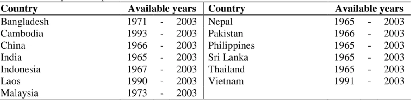
While most analyses of commodity prices focus on international prices, the framework proposed here allows for the study of country-specific producer data, which is better for determining the implications of policies on producers. Given that our theoretical model assumed the same production technology for all producers of the same good all over the world, we focused on a single commodity, rice, in a geographically and economically narrowed region, developing Asia. We collected producer price (IRRI website) and quantities harvested (FAOSTAT) for rice
16
in 13 Asian countries between 1965 and 20031 (Table 1). This choice is motivated by the need for
a homogenous region of study because our theoretical model assumes a common production technology for every country. Rice is an appropriate commodity for this kind of assumption given that there are few differences in the production systems used to cultivate rice in this region (except in Japan where production is highly mechanized and which is excluded from the sample).
Table 1 – Sample description
Country Available years Country Available years
Bangladesh 1971 - 2003 Nepal 1965 - 2003
Cambodia 1993 - 2003 Pakistan 1966 - 2003
China 1966 - 2003 Philippines 1965 - 2003
India 1965 - 2003 Sri Lanka 1965 - 2003
Indonesia 1967 - 2003 Thailand 1965 - 2003
Laos 1990 - 2003 Vietnam 1991 - 2003
Malaysia 1973 - 2003
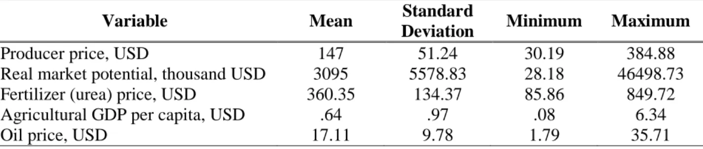
Exchange rates data were obtained from IMF-IFS. Market potentials calculated by Head and Mayer (2011) were obtained from the CEPII website. Equation (14) depended on a composite input price , which was not observed. We used available data on input prices (fertilizers, energy, and wages) as a proxy for this variable. However, input price data were scarce, especially for fertilizer and wages. To address this issue, we used agricultural gross domestic product per capita, computed as the agricultural GDP in local currency divided by the agricultural labor force (obtained from IRRI), as a proxy and filled in gaps in fertilizer prices (urea prices were obtained from IRRI) using data from other countries. We converted fertilizer prices into US dollars, computed a year specific mean, and filled gaps by converting those means into local currencies. Energy prices were approximated by the petroleum spot (US$/barrel) average crude price, converted into local currency. Details are provided in Table 2.
1
The study is narrowed to the 1965-2003 period due to the lack of availability of market access data prior to and after this interval (Head and Mayer 2011).
17
Table 2 - Descriptive statistics
Variable Mean Standard
Deviation Minimum Maximum
Producer price, USD 147 51.24 30.19 384.88
Real market potential, thousand USD 3095 5578.83 28.18 46498.73
Fertilizer (urea) price, USD 360.35 134.37 85.86 849.72
Agricultural GDP per capita, USD .64 .97 .08 6.34
Oil price, USD 17.11 9.78 1.79 35.71
Current literature takes advantage of the ability of the competitive storage model to reproduce (at least partially) some of the main characteristics of commodity prices: autocorrelation, skewness, and kurtosis. However, while these characteristics are typical of international prices, they are not shared by producer prices expressed in local currencies, which are not stationary as shown in Table 3. Therefore, our estimation results presented in Table 3 are based on the difference in the log of producer prices as presented in equations (13) and (14).
Table 3 – Fisher’s stationarity test for panel data (H0: unit root)
Variable - Statistic P-Value
Log of producer price, LCU 24.644 0.539
Log of producer price, USD 54.522 0.001
Difference in log of producer price, LCU 375.882 0.000
Difference in log of producer price, USD 378.244 0.000
Estimation results are presented in the first column of Table 4. As expected, all estimated coefficients were positive. Only exchange rates and market access coefficients were significantly different from zero. However, these coefficients have no economic interpretation in this framework due to the above-mentioned correlation with which is part of the error term. Some additional steps are necessary to obtain structural parameters, and . is obtained by
dividing the coefficient of by the coefficient of
, while requires additional calculations (with as the coefficient of variable in
the table of estimation results):
18
Table 4 - Estimation results
Dependent variable: (1) (2) (3) (4) 0.069** 0.071** 0.069** 0.083*** (0.024) (0.024) (0 .024) (0 .020) 0.427*** 0.433*** 0.429*** 0.532*** (0.044) (0.044) (0.045) (0 .066) 0.054 0.064 0.077 (0.058) (0 .053) (0 .056) 0.028 0.042 0.056 (0.036) (0.032) (0 .037) 0.146 0.160* 0.169** (0.085) (0.088) (0 .075) Observations 379 391 379 388 R-squared 0.236 0.232 0.234 0.287 (elasticity of substitution) 6.176** 6.080*** 6.217** 6.429** (2.039) (1.851) (2.058) (2.111)
(extent of returns to scale) .892*** .888*** 0.892*** 0.850***
(0.036) (0.036) (0.037) (0 .028)
-1.340*** -1.311*** -1.333*** -0.880***
(0.240) (0.236) (0 .244) (0 .232)
Robust standard errors clustered by country in parentheses. *** p<0.01, ** p<0.05, * p<0.1
First, was found to be 6.176, which is close to the estimate by Hummels (1999), who obtained an elasticity of approximately 5 with a standard deviation of about 2 for cereal products using a multi-sector model of trade. This estimate is also consistent with Armington elasticities proposed by McDaniel and Balistreri (2003), and classifies rice as a highly substitutable commodity. In this case, production shocks (and income changes) had rather small effects on price because of a high elasticity of substitution. Indeed, when is high, a weather shock in country has only a limited effect on producer prices in this country because consumers (in country and elsewhere) will substitute the variety of rice produced in country for varieties produced by other countries and other goods. Second, the estimate of supports non-increasing (but close to constant) returns to scale in agriculture (Bardhan 1973; Townsend,
19
Kirsten, and Vink 1998). Given these parameters, I estimated the elasticity of the final price
with respect to price expectations as . I obtained a surprisingly large effect of price expectations on market price of . Hence, a 1% increase in the forecasted price resulted in a fall of the market price by 1.34%, all things being equal. This result clearly highlights the importance of policies aimed at improving the quality of price information and stabilizing price expectations. Apart from these results, none of the included input prices appeared to have a significant effect, but they all had positive coefficients, in line with the predictions of the theoretical model.
Before further analyzing the various implications of these results, I used several methods to test their robustness. First, the scarcity of input price data was a major concern for the proposed estimation strategy. The results in columns 2–4 in Table 4 were obtained by dropping input prices in order to verify the stability of the coefficients of exchange rates and market potential variables, which are of crucial importance in the calculations of the structural parameters and and the elasticity of market price to price forecasts. If the estimated coefficients are sensitive to the inclusion or exclusion of one input price, then the omission of other input prices should bias the results. Only the exclusion of wage rate data significantly affected the coefficients of interest. This is by no means a surprise given the growing literature on the link between market access and wages. Many theoretical and empirical analyses have found a positive link between proximity to world markets and wages, which was confirmed by comparing the differences in coefficients between column 4 and all the other columns in Table 4 since the effect of increases when the wage rate drops. This change in the coefficient of
is counterbalanced by an increase in the coefficient of , so that neither
20
estimate of , the difference in column 1 was not significantly different from 0. In summary,
the omission of the wage rate did not significantly affect the estimates of the structural parameters of the theoretical model. The omission of other inputs did not significantly affect the market access or exchange rate coefficients. Given that proximity to the world market is not known to be correlated with any other input prices except wages, this specification should be robust to omitted input prices.
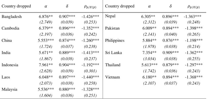
Another problem could arise if estimation results are sensitive to the exclusion of one specific country. Table 5 contains new estimates of equation (14) after dropping each country in turn. No country significantly affected the estimation results. In particular, the elasticity of the market price to changes in price forecast remained high, so further inquiries must be carried out to better understand how important price expectations are in price dynamics.
Table 5 – Robustness tests
Country dropped Country dropped
Bangladesh 6.876** 0.907*** -1.426*** Nepal 6.305** 0.896*** -1.363*** (2.749) (0.039) (0.253) (2.312) (0.039) (0.248) Cambodia 6.379** 0.896*** -1.352*** Pakistan 6.009** 0.894*** -1.398*** (2.197) (0.036) (0.242) (2.141) (0.040) (0.265) China 5.553*** 0.874*** -1.260*** Philippines 5.884** 0.876*** -1.198*** (1.724) (0.037) (0.238) (1.978) (0.038) (0.214)
India 5.671** 0.889*** -1.413*** Sri Lanka 7.354** 0.909*** -1.362***
(1.867) (0.038) (0.237) (3.034) (0.038) (0.255) Indonesia 7.961** 0.904*** -1.192*** Thailand 5.613*** 0.879*** -1.297*** (2.628) (0.039) (0.301) (1.742) (0.036) (0.243) Laos 6.048** 0.897*** -1.440*** Vietnam 6.180** 0.894*** -1.368*** (2.073) (0.038) (0.258) (2.107) (0.037) (0.243) Malaysia 5.536*** 0.880*** -1.328*** (1.604) (0.036) (0.251)
21
The present model does not allow us to decompose the error term between weather shocks and forecasting errors. However, equations (13) and (14) can give some information on the correlation between and .
First, according to equation (13), . Second, according
to equation (14), . We obtain: (15)
Reformulating this last equation gives:
(16)
Given this correlation, the objective was to simulate forecasting errors correlated with production shocks assuming different standard deviations for forecasting errors and find which provided the best fit to the data. To do so, I simulated both weather shocks and forecasting errors,
assuming that and and tested for different values for
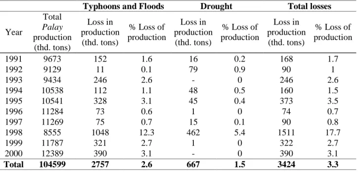
and . To do so, I chose and in accordance with the data presented in Table 6, the rice
losses due to climate shocks in the Philippines in the 90’s, and propose and
. Given these data, I chose values for comprised between 0.01 and 0.1. For each value
of , I tested for different values for (I imposed 2
.
2
22
Table 6 - Annual rice production and losses arising as a consequence of natural disasters in the
Philippines between 1991-2000
Typhoons and Floods Drought Total losses
Year Total Palay production (thd. tons) Loss in production (thd. tons) % Loss of production Loss in production (thd. tons) % Loss of production Loss in production (thd. tons) % Loss of production 1991 9673 152 1.6 16 0.2 168 1.7 1992 9129 11 0.1 79 0.9 90 1 1993 9434 246 2.6 - 0 246 2.6 1994 10538 112 1.1 48 0.5 160 1.5 1995 10541 328 3.1 45 0.4 373 3.5 1996 11284 73 0.6 1 0 74 0.7 1997 11269 75 0.7 15 0.1 90 0.8 1998 8555 1048 12.3 462 5.4 1511 17.7 1999 11787 321 2.7 1 0 322 2.7 2000 12389 390 3.1 - 0 390 3.1 Total 104599 2757 2.6 667 1.5 3424 3.3
Source: (Garcia-Rincon and Virtucio 2008)
Tables 7a and 7b present the distribution of changes in logged prices of simulated data based on rational price expectations using actual data. The characteristics of the simulated prices were not sensitive to the choice of . However, seemed to strongly determine the shape of the distribution of simulated prices. First, all simulated series underestimated the mean price change. This clearly highlights the need for the introduction of additional mechanisms (or at least input prices) in the model, such as inventories (Deaton and Laroque 1992) or monetary shocks
(Frankel 1986). Second, of the proposed values for , and generated the
best characteristics in terms of volatility (represented by the coefficient of variation), skewness, and kurtosis.
23
Table 7a – Summary statistics of observed and simulated price changes
Observed data Simulated data
Mean 0.070 0.055
Standard deviation 0.161 0.065
Coefficient of variation 2.285 1.162
Skewness 0.757 2.907
Kurtosis 6.791 19.070
Table 7b – Summary statistics of simulated price changes
Mean 0. 055 0.055 0.056 0.056 0.058 Std. dev. 0. 065 0.077 0.103 0.142 0.176 Coef. of var. 1.174 1.388 1.830 2.527 3.042 Skewness 2.857 2.178 0.970 -0.002 0.220 Kurtosis 18.822 14.596 6.386 3.385 4.032 Mean 0.055 0.055 0.054 0.054 0.057 Std. dev. 0.065 0. 076 0.099 0.121 0.169 Coef. of var. 1.172 1.370 1.820 2.230 2.972 Skewness 2.807 1.544 0.746 0.497 0.335 Kurtosis 18.100 8.989 6.031 4.573 3.563 Mean 0.056 0.056 0.056 0.056 0.055 Std. dev. 0.065 0.077 0.103 0.135 0.180 Coef. of var. 1.177 1.382 1.856 2.397 3.263 Skewness 2.736 1.811 1.087 -0.008 -0.195 Kurtosis 17.960 10.961 8.108 3.953 3.166
In order to determine which of these values for best fit the data, I generated QQ-plots
(Graph 1) of simulated series against actual data for different values of , when .
While simulated series with systematically underestimated positive and negative price
24
way. Even though it fails to predict the most severe price shocks, appears to be a good trade-off. In this case, producers have approximately a 50% chance of making prediction errors larger than 10% of the final price (Graph 2). This result clearly highlights the importance of price information in policies aimed at stabilizing prices.
Graph 1 - QQ-plot of simulated changes in log of prices – Rational expectations
Estimation and simulation results based on rational expectations reveal that price
expectation errors are large, which suggests that policies aimed at improving the quality of price
-. 5 0 .5 1 -.5 0 .5 1 -. 5 0 .5 1 -.5 0 .5 1 -. 5 0 .5 1 -.5 0 .5 1 -. 5 0 .5 1 -.5 0 .5 1 -. 5 0 .5 1 1 .5 -.5 0 .5 1
25
information would benefit rice producers in Asia. The problem of anticipation errors pointed in this study reinforces the current knowledge on the usefulness of the improvement of information systems through, for example, radio programs dedicated to farmers and detailing the situation of local, national and international markets (Svensson and Yanagizawa 2009). Furthermore, since futures markets synthesize available information on future market conditions into a unique price, futures hedging could not only help peasants protect themselves against price risk, but also provide them with a new source of information, the futures price, which might help improve the quality of price expectations.
Graph 2 – Histogram of simulated expectation errors with
(in proportion of the final price)
Conclusion
This article focuses on the role of price forecasting errors in a domestic price dynamics model based on international trade in varieties, rational expectations, and yield uncertainty. The theoretical model reveals that exchange rates, input prices, and price forecasts are the most influential determinants. Demand shocks and natural disasters have only a limited impact on
0 1 2 3 D e n si ty .5 1 1.5 2 random
26
prices because of the high elasticity of substitution between rice varieties. Empirical results support the model, confirming a high degree of substitution between rice varieties with an Armington elasticity of approximately 6 and non-increasing but close to constant returns to scale in the rice sector. Given these parameters, the model predicts that a 1% increase in price expectations results in a decrease in the market price by 1.34% and confirms the role of forecasts in price dynamics. The simulation exercise in this study was designed to determine the size of forecasting errors, and showed, assuming that forecasting errors are distributed as a log normal
distribution with and , that rice producers have a 50%
chance of making prediction errors larger than 10% of the final market price.
The policy implications of these findings are straightforward and twofold. First, increasing farmers access to information, such as through radio programs dedicated to providing farmers with specific information on market situations could benefit farmers by improving their access to information. Second, futures markets, which allow farmers to protect themselves against price fluctuations and provide predictions of future spot prices, may help stabilize price expectations, a necessary condition for sustainable growth.
However, the simulation exercise proposed in this paper reveals that this framework cannot fully explain the positive and negative price shocks that characterize agricultural price series. This result reveals the need for the introduction of other mechanisms in the model, such as competitive storage (Deaton and Laroque, 1992), monetary shocks (Frankel, 1986), or trade restrictions (Timmer, 2009), which have played an important role in recent price surges.
27
References
Armington, Paul S. 1969. « The Geographic Pattern of Trade and the Effects of Price Changes ».
Staff Papers - International Monetary Fund 16 (2): 179-201.
Bardhan, Pranab K. 1973. « Size, Productivity, and Returns to Scale: An Analysis of Farm-Level Data in Indian Agriculture ». Journal of Political Economy 81 (6): 1370-1386.
Boussard, Jean-Marc. 1996. « When risk generates chaos ». Journal of Economic Behavior &
Organization 29 (3): 433-446.
Boussard, Jean-Marc, and Sophie Mitra. 2011. « Storage and the Volatility of Agricultural Prices: a Model of Endogenous Fluctuations ». Économie rurale (321).
CRMG. 2008. The International Task Force on Commodity Risk Management in Developing Countries: Activities, Findings and the Way Forward. Commodity Risk Management Group. World Bank.
Deaton, Angus, and Guy Laroque. 1992. « On the Behaviour of Commodity Prices ». The Review
of Economic Studies 59 (1): 1-23.
———. 1996. « Competitive Storage and Commodity Price Dynamics ». Journal of Political
Economy 104 (5): 896-923.
———. 2003. « A model of commodity prices after Sir Arthur Lewis ». Journal of Development
Economics 71 (2): 289-310.
Ezekiel, Mordecai. 1938. « The Cobweb Theorem ». The Quarterly Journal of Economics 52 (2): 255 -280.
Frankel, Jeffrey A. 1986. « Expectations and Commodity Price Dynamics: The Overshooting Model ». American Journal of Agricultural Economics 68 (2): 344-348.
Galtier, Franck. 2009. How to manage food price instability in developing countries? Working Paper MOISA No 5.
Garcia-Rincon, Maria Fernanda and Felizardo K. Virtucio. 2008. « Climate Change in the Philippines: A Contribution to the Country Environmental Analysis ». WorldBank.
Country Environmental Analysis.
Gouel, Christophe. 2011. « Agricultural price instability: a survey of competing explanations and remedies». Journal of Economic Surveys Forthcoming.
Head, Keith, and Thierry Mayer. 2011. « Gravity, market potential and economic development ».
Journal of Economic Geography 11 (2): 281 -294.
Hommes, Cars H. 1994. « Dynamics of the cobweb model with adaptive expectations and nonlinear supply and demand ». Journal of Economic Behavior & Organization 24 (3): 315-335.
28
Hummels, David. 1999. Toward a Geography of Trade Costs. Center for Global Trade Analysis, Department of Agricultural Economics, Purdue University.
Lewis, W. Arthur. 1954. « Economic Development with Unlimited Supplies of Labour ». The
Manchester School 22 (2): 139-191.
Liefert, William M., and Suresh Persuad. 2009. The Transmission of Exchange Rate Changes to
Agricultural Prices. United States Department of Agriculture, Economic Research
Service.
Lovell, Michael C. 1986. « Tests of the Rational Expectations Hypothesis ». The American
Economic Review 76 (1): 110-124.
Mc Daniel, Christine A, and Edward J Balistreri. 2003. « A review of Armington trade substitution elasticities ». Economie Internationale 94-95 (2-3).
Muth, John F. 1961. « Rational Expectations and the Theory of Price Movements ».
Econometrica 29 (3): 315-335.
Nerlove, Marc. 1958. « Adaptive Expectations and Cobweb Phenomena ». The Quarterly Journal
of Economics 72 (2): 227-240.
Ramey, Garey, and Valerie A. Ramey. 1995. « Cross-Country Evidence on the Link Between Volatility and Growth ». The American Economic Review 85 (5): 1138-1151.
Svensson, Jakob, and David Yanagizawa. 2009. « Getting prices right: the impact of the market information service in Uganda». Journal of the European Economic Association 7 (2-3): 435-445.
Timmer, Peter C. 2009. Did Speculation Affect World Rice Prices? Agricultural and Development Economics Division of the Food and Agriculture Organization of the United Nations (FAO - ESA).