HAL Id: cea-02975826
https://hal-cea.archives-ouvertes.fr/cea-02975826
Submitted on 23 Oct 2020
HAL is a multi-disciplinary open access
archive for the deposit and dissemination of
sci-entific research documents, whether they are
pub-lished or not. The documents may come from
teaching and research institutions in France or
abroad, or from public or private research centers.
L’archive ouverte pluridisciplinaire HAL, est
destinée au dépôt et à la diffusion de documents
scientifiques de niveau recherche, publiés ou non,
émanant des établissements d’enseignement et de
recherche français ou étrangers, des laboratoires
publics ou privés.
Guided wave imaging of composite plates using passive
acquisitions by fiber Bragg gratings
Arnaud Recoquillay, Tom Druet, Simon Nehr, Margaux Horpin, Olivier
Mesnil, Bastien Chapuis, Guillaume Laffont, Oscar D'almeida
To cite this version:
Arnaud Recoquillay, Tom Druet, Simon Nehr, Margaux Horpin, Olivier Mesnil, et al..
Guided
wave imaging of composite plates using passive acquisitions by fiber Bragg gratings. Journal of
the Acoustical Society of America, Acoustical Society of America, 2020, 147 (5), pp.3565-3574.
�10.1121/10.0001300�. �cea-02975826�
Guided wave imaging of composite plates using
passive acquisitions by fiber Bragg gratings
Arnaud Recoquillay,1,a) Tom Druet,1 Simon Nehr,1Margaux Horpin,1 Olivier Mesnil,1 Bastien Chapuis,1 Guillaume Laffont,1and Oscar D’Almeida2
1CEA, LIST, Gif-sur-Yvette, France 2Safran Tech, Magny-Les-Hameaux, France
In this paper are presented imaging results of defects in composite plates using guided wave-based algorithms such as Delay and Sum and Excitelet. Those algorithms are applied to passive data, for which the signal corresponding to each emitter-receiver couple is recovered thanks to the cross-correlation of the ambient noise measured simultaneously by the two sensors. The transition to passive imaging allow the use of lighter sensors unable to emit ultrasonic waves such as Fiber Bragg Gratings sensors on optical fibers, which are used in this study. The imaging results presented here show the feasibility of active and passive imaging in composite plates using Fiber Bragg Gratings as receivers, reducing the impact of the acquisition system on the structure in the context of Structural Health Monitoring.
c
2020 Acoustical Society of America. [http://dx.doi.org/10.1121/10.0001300]
[XYZ] Pages: 1–11
Keywords: Elastic guided waves, composite plates, Fiber Bragg Gratings, Delay and Sum, Excitelet, passive imaging, Structural Health Monitoring
I. INTRODUCTION
Over the last decade, an increasing interest appeared for guided wave-based imaging methods in the context of Non Destructive Testing (NDT) as well as of Structural Health Monitoring (SHM). Indeed, guided waves enable 5
the inspection of a wide area of a structure with just a few sensors, reducing the inspection time and cost. In partic-ular, the use of less sensors allows to embed them in the structure, making SHM possible. However, SHM systems using classical sensors and algorithms may still be too big 10
of a burden for an industrial structure such as an aircraft. Hence the need of reducing this burden, for example by reducing the energy consumption of the sensors or their weight. To do so, passive acquisition methods seem a promising solution: they consist in recovering the impulse 15
response of the system composed of the medium and the sensors by treating the ambient noise measured simulta-neously at all sensors. The most common technique is the noise cross-correlation (Lobkis and Weaver,2001), which was used succesfully in various fields (Chehami et al., 20
2014; Davy et al., 2016; Roux et al., 2004; Sabra et al.,
2007, 2008;Shapiro and Campillo,2004). For structures subject to vibrations, it is then possible to recover data to which classical imaging algorithms can be applied with-out emitting energy. Furthermore, sensors such as Fiber 25
Bragg Gratings (FBG) on optical fibers, which are un-able to emit waves, can be used (Betz et al.,2003). Those sensors have previously been successfully used in combi-nation with piezoelectric transducers (PZT) for active
data acquisition (Betz et al.,2003;Takeda et al.,2005), 30
and more recently for passive data acquisition using noise cross correlation to recover the active signal first in seis-mology (Zeng et al., 2017) and then at ultrasonic fre-quencies for metallic plates (Druet et al.,2018).
The aim of this paper is to present passive guided-35
wave imaging in composite panels using only Fiber Bragg Gratings. Indeed, as passive methods do not need the emission of ultrasonic waves into the domain, this kind of imaging can be done with classic PZT sensors but also FBGs, opening the way of SHM systems of very low intru-40
siveness. In a first section is briefly recalled the principle of passive acquisition, before explaining the basis of Fiber Bragg Gratings sensors. Then, two guided wave imaging techniques are presented, namely Delay and Sum and Excitelet before presenting ultrasonic wave measurement 45
using FBGs. In the last section, experimental results ob-tained with these two algorithms on passive acquisitions for CFRP plates are presented. The first experiment was conducted using PZT sensors to check the feasibility of passive imaging in composite plates, and the full system, 50
using only FBG sensors, is tested in the second experi-ment.
II. ACTIVE AND PASSIVE ACQUISITION
The first step of any imaging algorithm is the data acquisition. For classical guided wave imaging algorithms 55
such as Delay and Sum, this step consists in successively emitting a wave with an actuator and measuring the sig-nal with all other sensors. This method is called, in the following, active acquisition. Another way to obtain
equivalent data is to measure the ambient noise at all 60
sensors simultaneously and then process those signals to reconstruct the data used in the imaging algorithm. This method is called, in the following, passive acquisition.
A few algorithms exist to retrieve the data from the ambient noise. The most known, which we will explain 65
in more details and use in the following, is the ambient noise cross-correlation (Lobkis and Weaver, 2001). An-other possibility is the passive inverse filter (Gallot et al.,
2012), which is well suited when many receivers are used. For example, this technique has been used for guided 70
wave tomography (Druet, 2017; Druet et al., 2019), for which more sensors need to be used to obtain a rele-vant image of the domain. As the passive inverse filter is based on the inversion of the impulse response matrix, it is a global process, which reconstructs all active signals 75
from all ambient noise simultaneously. This seems to al-low a better reconstruction, in particular if the ambient noise does not have a good distribution in space or fre-quency domain (Gallot et al.,2012), when many sensors are involved. Let us also mention the correlation of the 80
coda of the noise cross-correlation (Stehly et al., 2008), which may enhance the data’s reconstruction from the noise cross-correlation when many sensors are used, by enhancing the spatial distribution of the noise.
In this paper, we focus on the use of the cross-85
correlation of the ambient noise as this method has been more widely used until now and works well for any num-ber of sensors. Its principle and hypotheses are recalled in the following. For more details, the reader may refer to (Garnier and Papanicolaou,2009;Lobkis and Weaver, 90
2001;Roux et al.,2005). As the aim of this paper is the ultrasonic imaging of plates, we restrict ourselves to a domain in which linear elastic waves propagate. To the author’s best knowledge, the method for elastic waves has not yet been fully justified theoretically. Hence the justi-95
fication is given for scalar acoustic waves. Suppose that the ambient noise ϕ is a space-time stationary random field that is also delta correlated in space, which means that, for all t, τ > 0 and points x and y, the following relation holds
100
hϕ(x, t)ϕ(y, τ )i = K(x)δ(x − y)F (t − τ ), (1) where h·i denotes the ensemble average, K characterizes the spatial support of the sources and F is the normal-ized time correlation function, its Fourier transform be-ing linked to the spectral energy density of the ambient noise. We suppose in the following that the sources are 105
”well distributed” in space which means, depending on the nature of the domain Ω, that K ≡ 1 over a sufficient sub-domain (for more details, see (Garnier and Papani-colaou,2009)).
Let us now consider two sensors, at points x and 110
y acquiring the ambient noise within the time interval [0, T ], T > 0. Those signals are denoted Vxand Vy. The
cross-correlation C of these two signals is then
C(x, y, t; T ) = 1 T
Z T
0
Vx(τ )Vy(τ + t) dτ . (2)
Let Hxy be the impulse response of the system formed
of the finite domain, the sensor at x acting as a source 115
and the sensor at y acting as a receiver. Suppose that the noise sources have a good distribution in space, that is K ≡ 1, then
lim
T →+∞
dC
dt(x, y, t; T ) ∝ F ∗ [Hxy(·) − Hxy(−·)] (t), (3)
where ∗ denotes the convolution operation in time and · indicates the variable over which the operator, here the 120
convolution one, is taken. The convolution in time with F in (3) denotes the influence of the spectral density of the ambient noise: the impulse response’s reconstruction strongly depends on the time correlation of the noise, and so on the spectral energy density of the ambient noise. 125
In the following, as elastic waves propagate in the do-main of interest, we make the assumption that (3) is still relevant in this case. On a practical point of view, the quality of the data reconstruction will depend on a few parameters: first, the acquisition time T should be taken 130
large enough so that the cross-correlation converges. As will be seen in our applications, acquisition times of the order of at least one second should be used. The spatial repartition of the noise is also important: if the noise is not propagating in the axis going from x to y, then the 135
two signals Vxand Vy are not correlated and the
recon-struction will be poor. Likewise, if the energy is only propagating from x to y and not from y to x, for exam-ple if the domain has a low reverberation, then only the causal part of the signal will be correctly reconstructed. 140
As already stressed out, the frequency distribution of the noise is also to take into account, so that the signals’ en-ergy is sufficient for the frequencies of interest. Let us remark that to obtain (3), the assumption has been made that the transfer function of the sensor acting as a source 145
or as a receiver is the same, which in general is true. The combination of ambient noise cross-correlation and Fiber Bragg Gratings sensors, described in (Druet et al., 2018), allows for the determination of the pitch-catch response, that is the response of the structure for a 150
given sollicitation at one sensor and measured by another sensor, between two FBG sensors as if one was used as an emitter. This offers, on one hand, all the advantages of purely optical fiber sensing, such as dense wavelength multiplexing of the sensing points, immunity to and no 155
generation of Electro-Magnetic Interferences, compatibil-ity with harsh environments such as those involving high or low (cryogenic) temperatures, shock waves (detonic) and also ionizing radiations, as well as the possibility to drastically reduce the intrusiveness of the instrumenta-160
tion of any kind of structure thanks to reduced wirings. On the other hand, guided elastic waves offer a fine di-agnosis of the structure by enabling the detection, local-ization and sizing of defects as well as a full structure coverage.
III. GUIDED WAVE IMAGING TECHNIQUES
Many existing guided-wave based techniques could be used in combination with passive acquisitions. The only restrictions are the poor control over the recon-structed field, which prevent modal selection and, de-170
pending on the application, the frequency range for which the noise has enough energy. In this paper, two classi-cal methods are tested, namely Delay and Sum (DAS) (Michaels,2008) and Excitelet (Quaegebeur et al.,2011), as they were already tested in various cases for active 175
acquisitions (Kulakovskyi et al.,2019). Both algorithms were considered as they are representative of guided wave imaging techniques, using simple (DAS) or complex (Ex-citelet) models. Their principle is briefly recalled here-after.
180
In both cases, the algorithm is used for detecting a single defect in the plate. Suppose that reference data were acquired in a sound state, denoted sref
k for the
signal corresponding to the k-th emitter-receiver pair, 0 ≤ k < N . Note that sref
k (t) = C ∗F ∗H ref
xkykwith the no-185
tations of (3), where Href
xkykis the impulse response of the reference system for a source at xk and a receiver at yk
and C is a filter that can be added in the post-processing of the reconstructed signals. The signals corresponding to the state at the time of inspection are denoted sinspk . 190
Residual signals are computed by subtracting sref k to s
insp k
for each emitter-receiver pair. Then, in the case of DAS, the idea is, for each point x of the inspected area, to affect the value of the envelope of the residual signal cor-responding to the time of flight of the guided mode of 195
interest going from the emitter to the point x and then to the receiver. Indeed, if a defect is at this point x and the mode is not completely converted into another one, then a wave should be measured by the receiver at this time. By summing over all pairs, the coherence of the data is 200
verified and the points at which there is a higher prob-ability of presence of the defect are highlighted. More precisely, the Delay and Sum algorithm is the following: 1. Computation of the envelope of the residual signal
for each pair: 205
˜
sresk (t) = |H(sinspk (t) − srefk (t))|, (4) where H denotes the Hilbert transform.
2. For each point x of the inspected area, computation of the corresponding time of flight for each pair:
Tk(x) = |x − xe k| cg(θ(xek, x)) + |x r k− x| cg(θ(x, xrk)) , (5) where xe k(x), respectively x r
k(x), denotes the
posi-tion of the emitter, respectively the receiver, for 210
the k-th signal, θ(x, y) is the angle formed by y − x and the positive horizontal axis and cgdenotes the
energy velocity of the mode of interest, which will be discussed in the following.
3. Extraction of the value of the envelope correspond-215
ing to the time of flight and summation over all
signals: PDAS(x) = N −1 X k=0 ˜ sresk (Tk(x)). (6)
The strong hypothesis, and the main weakness of this method, is that it considers one single mode, propagat-ing at a fixed energy velocity. It means that no mode 220
conversion by the defect is taken into account, and that other emitted modes may perturb the imaging process. Furthermore, it is well known that guided waves have a dispersive behavior, which means that their energy ve-locity depends on the frequency. To use this method, it 225
is then recommended to consider a frequency range for which the dispersion of the mode of interest is low, or to consider a narrow-band excitation, which will reduce the resolution as the support in time of the signal will be large.
230
The Excitelet algorithm is based on the same ideas but compares, thanks to a correlation, the residual sig-nal to the theoretical one obtained when propagating the wave obtained for a given source from the emitter to the considered point and then to the receiver. More precisely, 235
the steps of the algorithm are the following:
1. Computation of the residual signal for each pair: sresk (t) = sinspk (t) − srefk (t). (7) 2. Computation of the theoretical signal for each pair: as the defect is considered as a point scatterer, the theoretical field scattered by this point is equal, in 240
the frequency regime, to the Green’s function of the plate time the incident field emitted by the source: sthk (t) = F−1[Vkr(x, ·)Vke(x, ·)] (t), (8) where F−1 is the inverse Fourier Transform, and Ve
k and V r
k are respectively the wave emitted by
245
the emitter and measured by the receiver of the k-th pair in the frequency regime. More precisely,
Vke(x, ω) = Z R2 G(x, y, ω)f (y) dy U (ω), (9) Vkr(x, ω) = Z R2
g(y)TG(y, x, ω) dy, (10) G being the Green’s function of the problem, f the source function in space, g the measurement func-tion and U the Fourier transform of the excitafunc-tion 250
signal. Note that f and g are implicitly supposed compactly supported on the support of the sensor, giving meaning to the integrals. Note also that, as the considered problem is the elastodynamic one, G is a matrix whereas f and g are vectors but the 255
signal is scalar in (8).
3. Computation of the correlation between the resid-ual signal and the theoretical one and summation over all signals:
PExcitelet(x) = N X k=0 Z R sresk (t)sthk (t) dt. (11)
Both algorithms use the same inputs, that is signals at 260
the inspection time and reference ones. Unlike DAS, Ex-citelet takes into account the guided waves dispersion through the computation of the theoretical signal. How-ever, as the model used is more precise, a good knowl-edge of the parameters of the sample is mandatory. The 265
use of a correlation in time also implies that the emitted signal should be short to increase the resolution. The computation of the theoretical signal may be time and memory-consuming in complex cases such as composite materials. To reduce it, a far-field approximation of the 270
Green’s function may be used in expressions (10) or only some modal components of the Green’s function can be selected. With those two approximations, one obtains G(x, y, ω) ≈ H1(i)(km(ω, θ)|x−y|), where H
(i)
1 is the
Han-kel function of first order and i-th kind, i = 1, 2 depend-275
ing on the convention used in the Fourier transform, km
is the wavenumber of the considered mode and θ is the angle of the vector x − y.
Finally, let us point out that, for passive acquisitions, the Fourier transform of the excitation signal U can be 280
imposed in post processing, enabling the optimization of the imaging results.
In all the following, the imaging results correspond to normalized indicator functions, that is Pa(x)/ max Pa,
where a is either DAS or Excitelet. 285
IV. ULTRASONIC WAVE MEASUREMENT USING FIBER BRAGG GRATINGS
Usually employed to measure temperature and strain, Fiber Bragg gratings are increasingly attracting researchers studying ultrasonic guided waves-based imag-290
ing methods for SHM applications. Indeed, their low in-trusiveness and multiplexing capabilities (both spectrally and temporally) make FBGs an attractive alternative to piezoelectric elements as acoustic receivers. While dense wavelength multiplexing of tens of FBGs on a single op-295
tical fiber is commonly used in Telecommunications and even in Sensing applications, its immediate transposition to the case of FBGs used as acoustic receivers is still challenging. Active or passive acquisitions of ultrasonic signals using FBGs sensors require both a sampling fre-300
quency ranging from kHz to MHz levels while preserv-ing their multiplexpreserv-ing capabilities and a high sensitivity to the strain variations induced by the ultrasonic sig-nals propagating across composite plates. In this study, we have developed a monitoring system dedicated to 305
wavelength-multiplexed FBG used as acoustic receivers. The principle of this measurement system relies on an edge filtering technique. The basic idea of the technique is the use of a tunable laser source per FBG acoustic receiver. For a given Bragg wavelength, the lasing wave-310
length emitted by an external cavity wavelength-tunable laser source is adjusted to the midpoint of one edge of the Bragg peak. Any shift of the Bragg wavelength will modulate the transmitted/reflected optical power. This demodulation scheme is commonly referred to as 315
”edge filtering” technique (Melle et al., 1992). Hence
the sampling rate at which each FBG is demodulated does not depend on the acquisition speed of a given spectral analyzer but rather simply on the band pass of both the pigtailed photodetectors and the associated 320
transimpedance electronic. This straightforward demod-ulation method allows adjusting easily the measurement frequency by simply changing the cutoff frequency of the transimpedance electronic but at the expense of the rather low degree of integration due to the need of one 325
tunable laser source per FBG acoustic receiver. Multi-plexing the FBG acoustic receivers simply requires to cas-cade several tunable lasers and to inject their optical sig-nals to the fiber containing the sensors thanks to an all-fiber wavelength multiplexer. A similar component po-330
sitioned before the photodetectors separates the signals reflected by each FBG. In this study, a transimpedance circuit with cutoff frequencies of 1 MHz has been realized in order to handle four photodetectors simultaneously.
V. EXPERIMENTAL RESULTS
335
A. Passive acquisition using piezoelectric transducers
A first experiment was carried out using classic piezo-electric transducers of diameter 18 mm in order to check the feasibility of using passive acquisitions to image com-posite plates. The used sample was a 1000 × 600 × 5.75 340
mm3CFRP plate having 21 plies, all oriented in the same
direction. Its material parameters are given in tableI.
Table I. Material parameters of the CFRP plates
E1= E2 (MPa) E3 (MPa) ν12 ν13= ν23 G12 (MPa) G13= G23 (MPa) ρ (kg.m−3) 65700 4500 0.03 0.3 5100 3750 1550
The ambient noise was created thanks to a com-pressed air flow moved randomly over the whole surface of the plate during the acquisition. Eight piezoelectric 345
transducers were placed on a circle of radius 200 mm. This radius was chosen so that reflections on the border of the plate are measured after an incident wave coming from the opposite sensor for frequencies around 20 kHz, the measured ambient noise having a significant spec-350
tral energy density between 10 kHz and 80 kHz. The ambient noise was measured simultaneously on the eight sensors for 10 seconds at a sampling rate of 1 MHz. As already mentioned in sectionIII, the quality of the im-age obtained with DAS or Excitelet is strongly linked to 355
the excitation signal. Here the signal reconstructed from the ambient noise cross-correlation has been filtered to obtain signal characteristics appropriate for those imag-ing algorithms. More precisely, two different filters were tested: a Hann filter of central frequency 20 kHz and of 360
bandwidth 20 kHz and one of central frequency 45 kHz and of bandwidth 70 kHz. For both algorithms, only the A0 mode was considered and, in the case of DAS, the
(a) first defect
(b) second defect
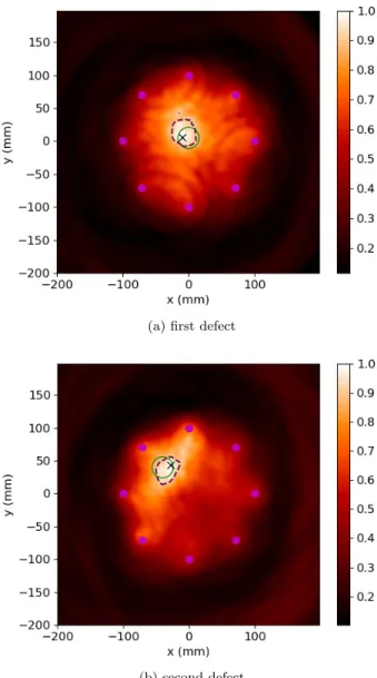
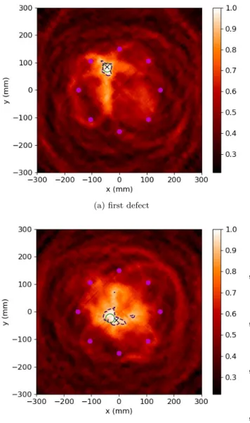
Figure 1. (color online) DAS applied to passive acquisitions with PZT, frequency range: 10-30 kHz.
energy velocity is taken at the central frequency of the considered filter. Synthetic defects were obtained using 365
a pair of magnets of diameter 32 mm, placed for the first defect at (0, 5), which is a slightly off-centered position, and at (−40, 40) for the second one. In all the following images, the black dashed lines are contour lines corre-sponding to the value 0.9, added as an illustration. The 370
green circle is the true shape of the defect whereas the black cross is the location of the maximum amplitude of the cartography. First, the imaging results for DAS are shown in figures1 and2.
In both cases, the localizations of the defect are well 375
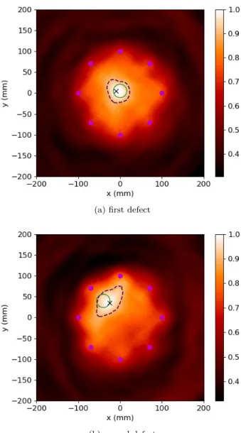
retrieved. It should be noted that the image has a better accuracy in figure2than in figure1, that is the high am-plitude spot is smaller in figure2, enabling a better
local-(a) first defect
(b) second defect
Figure 2. (color online) DAS applied to passive acquisitions with PZT, frequency range: 10-80 kHz.
ization of the defect. This comes from the low dispersion of the A0 mode in this frequency range, inducing a
bet-380
ter resolution for a bigger bandwidth as the wavepacket is shorter in time.
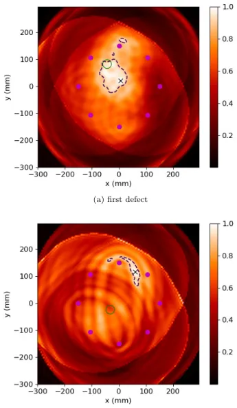
The imaging results corresponding to Excitelet are presented figures 3 and 4. The localization is again of good quality, even though the 0.9 contour is wider in 385
this case. This may come from a greater sensitiveness to the noise in the passive reconstruction: as will be seen inV B, Excitelet is more precise as long as the data are of good quality. Finally, in tableII is given the distance between the center of the defect and the maximum of 390
the cartography. Except for the case of low frequency DAS, the distance is lower than the radius of the defect,
(a) first defect
(b) second defect
Figure 3. (color online) Excitelet applied to passive acquisi-tions with PZT, frequency range: 10-30 kHz.
which is the best result possible given the point scatterer assumption of the algorithms.
395
B. Passive acquisition using Fiber Bragg Gratings on optical fibers
The acquisition using FBG sensors was done on a 400
1010 × 610 × 2.2 mm3CFRP plate having 8 plies, all
ori-ented in the same direction. Its material parameters are the same as the previous plate, given in table I. Eight FBG sensors were placed on the surface of the plate on a circle of radius 150 mm centered at the middle of the 405
plate. Due to the used acquisition device, the signals of only four FBG could be recorded simultaneously. As the ambient noise needs to be recorded simultaneously
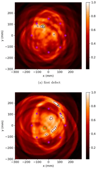
(a) first defect
(b) second defect
Figure 4. (color online) Excitelet applied to passive acquisi-tions with PZT, frequency range: 10-80 kHz.
on the sensors to recover the impulse response from the cross-correlation, this means that only a part of the data 410
was obtained (see figure5). Only 24 different signals can then be reconstructed, where 56 different pairs exist and were used in the previous section. Note that all FBGs are oriented toward the center of the circle in order to maximize their sensitivity in the region of interest (Betz
415
et al., 2003). Defects were again simulated thanks to a pair of magnets of diameter 32 mm, placed at (−44, 82) for the first position and (−32, −24) for the second one. The noise was measured during 50 seconds as to ensure a good reconstruction of the signals. The Fiber Bragg 420
Gratings are 5 mm long with a reflectivity greater than 97%. They were photowritten in a polyimide-coated
ger-Table II. Distance of the maximum to the center of the defect, PZT case
Algorithm case wavelength (mm)
distance (mm) DAS low frequency, defect 1 31 25
low frequency, defect 2 31 18 high frequency, defect 1 20 10 high frequency, defect 2 20 13 Excitelet low frequency, defect 1 31 5
low frequency, defect 2 31 7 high frequency, defect 1 20 10 high frequency, defect 2 20 16
Figure 5. Scheme of the acquisition setup using FBGs
manosilicate singlemode optical fiber using a KrF laser emitting at 248 nm and a Talbot interferometer.
The images obtained using DAS are presented figures 425
6and7. In this case, the obtained images do not enable to recover the position of the defects. An approximate position of the first defect may be recovered for both bandwidth, but the second one is not retrieved. In both cases, a strong noise exists in the images. Let us recall 430
that less than half the data used in the previous section were available in this case, which may explain for a great part the poor results.
Applying Excitelet, figures 8 and 9, the results are more satisfying: even though there still is noise in the 435
images, the locations of the defect are properly recon-structed, with a better accuracy for the central frequency of 45 kHz as expected. Indeed, in figure8, the algorithm detects the presence of a defect but its position and size are not retrieved. This result is the first demonstration 440
of the possibility of using FBG sensors with a passive acquisition for guided wave imaging of composite pan-els. The imaging results obtained with both algorithms are of the same quality using FBG or PZT, even though less than half the signals used in the PZT case could be 445
acquired with the FBGs. It is interesting to note that both algorithms may be used with passive data as DAS
(a) first defect
(b) second defect
Figure 6. (color online) DAS applied to passive acquisitions with FBG, frequency range: 10-30 kHz.
is easy to use and does not require a high knowledge of the wave propagation in the plate whereas Excitelet re-quires a higher knowledge leading to a higher accuracy. 450
Once again, the distance between the center of the de-fect and the maximum of the cartography is summarized in table III. In this case, as expected, the maximum is in general far from the defect. It should nevertheless be noted that the results are generally better for the high 455
frequency filter, which is expected, and that the results ar particularly good in this case for Excitelet.
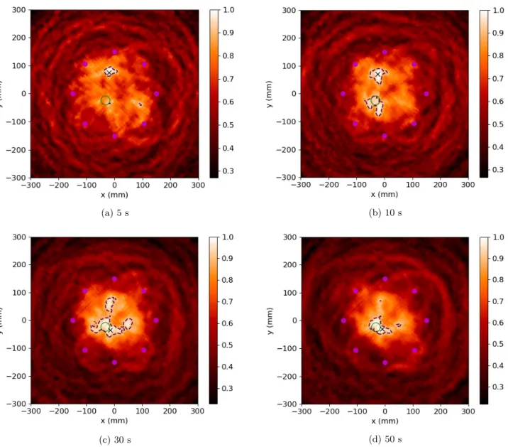
Before concluding, the imaging results of Excitelet are plotted in figure10for various noise acquisition time. It can be seen that the image’s resolution increases with 460
the acquisition duration due to the convergence of the cross-correlation of the ambient noise. It seems that,
(a) first defect
(b) second defect
Figure 7. (color online) DAS applied to passive acquisitions with FBG, frequency range: 10-80 kHz.
with the current system, an ambient noise acquisition of 30 seconds is necessary to have a sufficient signal re-construction, enabling the localization of a defect. But 465
this value depends on various factors, among which are: the frequency content of the noise source, the frequency dependent transfer function of the sensors and of the ac-quisition system. For example, stronger analogical fil-tering of the noise around the bandwidth of interest, or 470
equivalently a noise with a bandwidth closer to the one of interest, can help to have a better resolution in the reconstruction. As the noise source depends strongly on the application and is a parameter on which the user has no control, tailoring the acquisition system towards the 475
expected frequency content of the noise may be a satis-fying solution.
(a) first defect
(b) second defect
Figure 8. (color online) Excitelet applied to passive acquisi-tions with FBG, frequency range: 10-30 kHz.
VI. CONCLUSION
In this article has been shown the feasibility to image 480
composite CFRP plate with elastic guided wave imaging algorithms on passive acquisitions thanks to FBG sen-sors. Many parameters need to be thoroughly studied to determine in which configurations this approach can be used and several ways of improvement are being investi-485
gated: first of all, not all signals could be reconstructed with the current acquisition system, limited to only 4 parallel FBG channels. The development of a system with more channels is undergoing at CEA and will lead to improved imaging results in the future. Another pa-490
rameter is the angular sensitivity of the FBG sensors: the measurement depends on the angle between the inci-dent wave on the gratings and its direction. Even though
(a) first defect
(b) second defect
Figure 9. (color online) Excitelet applied to passive acquisi-tions with FBG, frequency range: 10-80 kHz.
the direction of the gratings were chosen as to optimize the measurements in the region of interest in our exper-495
iment, the imaging algorithms used does not take that into account. They should be adapted to take into ac-count this variable sensitivity. Finally, other methods to reconstruct the active signal from the ambient noise could be tested, such as the passive inverse filter (
Gal-500
lot et al., 2012), which may improve the reconstruction, especially when many sensors are used.
This first demonstration of a guided-wave-based imaging of composite panels using only FBG sensors opens the way to lightweight SHM systems with a very 505
low intrusiveness. Other declinations can be anticipated for configurations that highly benefit of the other
advan-Table III. Distance of the maximum to the center of the defect, FBG case
Algorithm case wavelength (mm)
distance (mm) DAS low frequency, defect 1 31 79
low frequency, defect 2 31 167 high frequency, defect 1 20 6 high frequency, defect 2 20 235 Excitelet low frequency, defect 1 31 57
low frequency, defect 2 31 80 high frequency, defect 1 20 3 high frequency, defect 2 20 23
tages of the FBGs, such as their high temperature or radiation resistance.
510
Betz, D. C., Thursby, G., Culshaw, B., and Staszewski, W. J. (2003). “Acousto-ultrasonic sensing using fiber Bragg gratings,” Smart Materials and Structures 12(1), 122.
Chehami, L., Moulin, E., De Rosny, J., Prada, C., Bou Matar, O., Benmeddour, F., and Assaad, J. (2014). “Detection and lo-515
calization of a defect in a reverberant plate using acoustic field correlation,” Journal of applied Physics 115(10), 104901. Davy, M., De Rosny, J., and Besnier, P. (2016). “Green’s
func-tion retrieval with absorbing probes in reverberating cavities,” Physical review letters 116(21), 213902.
520
Druet, T. (2017). “Tomographie passive par ondes guid´ees pour des applications de contrˆole sant´e int´egr´e,” Ph.D. thesis, Univer-sit´e de Valenciennes et du Hainaut-Cambr´esis.
Druet, T., Chapuis, B., Jules, M., Laffont, G., and Moulin, E. (2018). “Passive guided waves measurements using fiber Bragg 525
gratings sensors,” The Journal of the Acoustical Society of Amer-ica 144(3), 1198–1202.
Druet, T., Recoquillay, A., Chapuis, B., and Moulin, E. (2019). “Passive guided wave tomography for structural health monitor-ing,” Journal of the Acoustical Society of America .
530
Gallot, T., Catheline, S., Roux, P., and Campillo, M. (2012). “A passive inverse filter for Green’s function retrieval,” The Journal of the Acoustical Society of America 131(1), EL21–EL27. Garnier, J., and Papanicolaou, G. (2009). “Passive sensor imaging
using cross correlations of noisy signals in a scattering medium,” 535
SIAM Journal on Imaging Sciences 2(2), 396–437.
Kulakovskyi, A., Mesnil, O., Lh´emery, A., Chapuis, B., and d’Almeida, O. (2019). “Defect imaging in layered composite plates and honeycomb sandwich structures using sparse piezo-electric transducers network,” 1184(1), 012001.
540
Lobkis, O. I., and Weaver, R. L. (2001). “On the emergence of the Green’s function in the correlations of a diffuse field,” The Journal of the Acoustical Society of America 110(6), 3011–3017. Melle, S. M., Liu, K., and Measures, R. (1992). “A passive wave-length demodulation system for guided-wave bragg grating sen-545
sors,” IEEE Photonics Technology Letters 4(5), 516–518. Michaels, J. E. (2008). “Detection, localization and
characteri-zation of damage in plates with an in situ array of spatially distributed ultrasonic sensors,” Smart Materials and Structures 17(3), 035035.
550
Quaegebeur, N., Masson, P., Langlois-Demers, D., and Micheau, P. (2011). “Dispersion-based imaging for structural health mon-itoring using sparse and compact arrays,” Smart Materials and Structures 20(2), 025005.
Roux, P., Kuperman, W., and Group, N. (2004). “Extracting co-555
(a) 5 s (b) 10 s
(c) 30 s (d) 50 s
Figure 10. (color online) Excitelet applied to reconstructed signals for various noise acquisition durations.
The Journal of the Acoustical Society of America 116(4), 1995– 2003.
Roux, P., Sabra, K. G., Kuperman, W. A., and Roux, A. (2005). “Ambient noise cross correlation in free space: Theoretical ap-560
proach,” The Journal of the Acoustical Society of America 117(1), 79–84.
Sabra, K. G., Conti, S., Roux, P., and Kuperman, W. (2007). “Passive in vivo elastography from skeletal muscle noise,” Ap-plied physics letters 90(19), 194101.
565
Sabra, K. G., Srivastava, A., Lanza di Scalea, F., Bartoli, I., Rizzo, P., and Conti, S. (2008). “Structural health monitoring by ex-traction of coherent guided waves from diffuse fields,” The Jour-nal of the Acoustical Society of America 123(1), EL8–EL13. Shapiro, N. M., and Campillo, M. (2004). “Emergence of broad-570
band Rayleigh waves from correlations of the ambient seismic noise,” Geophysical Research Letters 31(7).
Stehly, L., Campillo, M., Froment, B., and Weaver, R. L. (2008). “Reconstructing Green’s function by correlation of the coda of the correlation (C3) of ambient seismic noise,” Journal of Geo-575
physical Research: Solid Earth 113(B11).
Takeda, N., Okabe, Y., Kuwahara, J., Kojima, S., and Ogisu, T. (2005). “Development of smart composite structures with small-diameter fiber Bragg grating sensors for damage detection: Quantitative evaluation of delamination length in CFRP lami-580
nates using Lamb wave sensing,” Composites science and tech-nology 65(15-16), 2575–2587.
Zeng, X., Lancelle, C., Thurber, C., Fratta, D., Wang, H., Lord, N., Chalari, A., and Clarke, A. (2017). “Properties of noise cross-correlation functions obtained from a distributed acoustic sensing 585
array at Garner Valley, California,” Bulletin of the Seismological Society of America 107(2), 603–610.
![[PDF] Supports de cours sur les Bases du langage XML | Cours informatique](data:image/gif;base64,R0lGODlhAQABAIAAAP///wAAACH5BAEAAAAALAAAAAABAAEAAAICRAEAOw==)