OATAO is an open access repository that collects the work of Toulouse
researchers and makes it freely available over the web where possible
Any correspondence concerning this service should be sent
to the repository administrator:
[email protected]
This is an author’s version published in:
http://oatao.univ-toulouse.fr/24155
To cite this version:
Varais, Andy and Roboam, Xavier and Lacressonnière,
Fabien and Turpin, Christophe and Cabello, J.M. and Bru,
Eric and Pulido, Joachin Scaling of wind energy conversion
system for time-accelerated and size-scaled experiments.
(2019) Mathematics and Computers in Simulation, 158.
65-78. ISSN 0378-4754
Official URL:
https://doi.org/10.1016/j.matcom.2018.05.015
Scaling
of wind energy conversion system for time-accelerated and
size-scaled
experiments
A. Varais
a,∗,
X. Roboam
a,
F. Lacressonnière
a,
C. Turpin
a,
J.M. Cabello
b,
E. Bru
a,
J. Pulido
aaLAPLACE, Université de Toulouse, CNRS, INPT, UPS, France
bLAC, Facultad de Ciencias Exactas, Ingeniería y Agrimensura, Universidad Nacional de Rosario, Argentina
Abstract
This paper presents a scaling methodology based on dimensional analysis and applicable to systems’ mathematical models. The main goal of this research is to propose time-accelerated and size-scaled HIL (Hardware In the Loop) experiments, while keeping similarity with respect to the dynamics of the original system. The scaling process is presented using a simple wind turbine model. The scaling method is validated through simulations in which a wind turbine model and an electrochemical battery model are connected together. Finally, an experimental real-time validation is performed using physical emulators.
Keywords: Wind system; Similarity; Hardware-in-the-loop (HIL); Time acceleration; Dimensional analysis
1. Introduction
The global energy landscape is constantly evolving. Emergence of new environmental objectives, the development of renewable energies and new uses of electricity (heat pump, electric car, etc.) require modernization of electricity networks. This latter issue is coupled with the optimization of the management of electrical production which promises energy savings. In this framework, stages of modelling, simulation and experimentation become key issues.
Nevertheless, the experimental phase can be difficult when systems are complex. The related cost is huge especially for high power systems as for wind production. Furthermore, environment dynamics (solar irradiation, thermal conditions, wind speed) have to be reproduced, which usually lead to long time range of experiments. Therefore, it is advisable to use scaled models both to decrease the experiment cost and for “time acceleration”, this latter concept
∗
Corresponding author.
E-mail addresses: [email protected] (A. Varais), [email protected] (X. Roboam),
[email protected] (F. Lacressonnière), [email protected] (C. Turpin), [email protected] (J.M. Cabello), [email protected] (E. Bru), [email protected] (J. Pulido).
being one of the key issues of this paper. As numerical simulations make possible to deduce the characteristics of the phenomena in real size, reduced scale physical emulation based on HIL experiments minimizes the risks associated with the experiments and decreases associated costs [2,4]; such process aims at experimentally validating the simulations especially dynamic (real time) aspects related to control and management of power systems.
There are various studies that deal with the development of sized-scale HIL simulator, and different methodologies are used in order to achieve system scaling. The power level adjustment between reduced- and full-scale systems can be achieved through adaptation of coefficients [2,5,15]. Coupled with an adequate control, this method allows reproducing at small scale the behaviour of certain full-scale system aspects. Some authors developed a 20 kW small-scale simulator to study the control dynamics of the inverter for more powerful wind turbine, using design criteria [14,17,18]. Unfortunately, these criteria are specific to wind turbine and not applicable to other systems. Furthermore, the developed simulators show similar trends between real and scaled systems, but on a limited number of aspects. To obtain a reduced-scale HIL simulator which shall be representative of a large number of aspects of the real system (in the model used validity domain), all variables of the system have to be taken into account and to be recalculated in order to obtain similar behaviours for reduced- and full-scale systems. In [3], Belouda et al. use a similitude sizing principle based on the geometric variations study of equipment [12]. This approach allows a modification of the wind turbine power produced as a function of the geometric elements evolution. In order to establish similitude relationships, some assumptions are necessary. Therefore, unlike dimensional analysis used in this paper, some scale factors are initially set, which removes degrees of freedom.
The size-scale models based on similitude theory are also widespread in other scientific areas such as fluid mechanics of civil engineering. This theory has played important role in experimental mechanics up to the present as summarized in the comprehensive review by Coutinho et al. [10]. In electrical engineering, dimensional analysis is starting to be used to develop scaled-model [11,19]. Moreover, these similarity models also allow envisaging simulated experimentation (concept of physical emulation) in “compacted virtual time” which makes more efficient (being more rapid) the validation process: as far as we know this “ virtual time acceleration concept” has not be seen in the state of the art and is then an original proposition. The issues of similarity will have to achieve relevant scale reductions and so they are as useful in sizing models for system engineering as for models built into physical emulators.
The laws of physics are invariant with respect to any change of unity. This invariance property is essential. It allows defining the behaviour of a physical system by a complete set of dimensionless variables formed by relevant physical variables. Then it is possible to compare the systems with each other by comparing their dimensionless quantities. The Vaschy–Buckingham theorem [8] (or Π theorem), basic theorem of dimensional analysis, allows setting how many independent dimensionless numbers can be constructed in a physical problem that involves n variables.
The objective of this paper is to develop a HIL simulation of a wind energy conversion system and realize a time-accelerated experiment. First of all, the similitude theory and the general method of system scaling are introduced. Afterwards, a simulation analysis of wind energy conversion system (in which the similitude theory is used) is presented. In this simulation, the wind turbine is connected to the grid with a storage device (lithium-ion battery). Finally, the overall wind energy conversion system is emulated in a scaled test bench in “virtual compacted time” and the result is compared to real-time emulation.
2. Similitude theory
The purpose of dimensional modelling is to carry out experiments on a scaled-model system, and then to be able to project the obtained results on the full-scaled system.
Similitude theory is a branch of engineering science concerned with establishing the necessary and sufficient conditions of similarity among phenomena. According to this theory, two systems have the same behaviour (under the same experimental conditions) if their dimensionless variables have the same values, respectively [6]. This property allows studying the behaviour of a system by carrying out experiments on another system (here an emulated system), similar to the first, but with a more practical (reduced and cost effective) physical scale.
Therefore, the similitude theory has the following objectives: • Proposing independent dimensionless numbers (calledπ-groups); • Simplifying basic equations by removing irrelevant variables;
• Establishing criteria to be fitted for a scale experiment in order to be representative of a full-scale phenomenon; • Providing the scale change relationships between “scale one” and reduced scale experiments.
The Buckingham theorem allows studying a physical problem with n variables to a problem of dimension k = n −r expressed in terms of dimensionless numbers (with r the number of independent physical dimensions).
2.1. Dimensional Analysis
In engineering and science, dimensional analysis is related to the relationships between different physical quantities by identifying their fundamental dimensions. It is a powerful tool widely used for scale model calculation [7,20].
Nondimensionalization procedure is started by identifying the number n of relevant physical quantities (variables and parameters) used to describe the behaviour of the system. Secondly, setting their units in the international MKSA system is also necessary, which allows calculating the number r of independent fundamental dimensions. r also represents the number of available degrees of freedom (i.e. the number of independent variables that can be scaled).
Examples:
• transforming the newton [N] unit in the MKSA system: according to the weight formula P[N] = m[kg] × g[m/s2], the newton is expressed in fundamental units as follows: 1N = 1 kg.m.s−2.
• transforming the joule [J] unit in the MKSA system: according to the formula of kinetic energy E [J] =
1
2m[kg].v
2[m2/s2]: 1J = 1 kg.m2.s−2
The number k ofπ-groups necessary to represent the system studied is calculated as follows [4]:
k = n − r (1)
From this information, a table composed of 4 matrices A, B, C, D is constructed.
• The entries of matrices A and B are the exponents associated with the fundamental dimensions of the unit of the parameter/variable.
• Repeating parameters can be chosen arbitrarily provided that the matrix A is invertible. However, it is wise to choose the parameters that will be scaled to simplify the calculations.
• The matrix D must be of the simplest form possible in order to have the simplest possibleπ-groups. It is usual to use the identity matrix which makes it possible to have a decoupling between π-groups and the parameters/variables of the model to be reduced: eachπ-group depends on a single parameter/variable as well as on certain repeating parameters.
• Matrix C is calculated as follows: C = −D(A−1B)T
(2) Details can be found in [20].
Then this table allows setting the expressions of the different π-groups which are a combination of a single parameter/variable and repeating parameters.
Some examples of this matrix derivation are provided in Section3. 2.2. Scale factor
In order to determine the scaled model parameters, we introduce the notion of “scale factor”. A scale factor Sx
always refers to a particular physical variable x and is defined as the quotient of the scaled variable and the original variable:
Sx=
xscaled
xor i gi nal
(3) Each variable or parameter corresponds to a scale factor which can be expressed directly from the π-group associated to it through a relation that forms a particular model called «Model Law».
As mentioned before, two systems of the same kind have the same behaviour (under the same experimental conditions) if their dimensionless variables have the same values, respectively. Consequently the scale factors of π-groups must be equal to 1 in order for the reduced model to have the same dynamics as the original model. Thus, the scale factor of a variable can be determined from the expression of theπ-groups associated with it (this expression will be a function of the repeating parameters).
(1) Determination of relevant physical variables; (2) Dimensional analysis (MKSA units);
(3) Choice of variables to be scaled (repeating parameters); (4) Calculation ofπ-groups;
(5) Determination of scale factors;
(6) Calculation of scaled model parameters.
3. Application to a wind energy conversion system
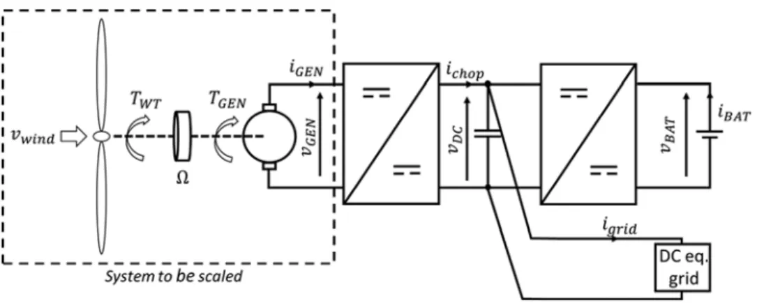
In order to present the similitude theory, a simplified case study that has relatively few physical variables has been selected; for example, actual generator — power electronic association has been replaced by an “energetically equivalent” DC machine supplying a DC–DC chopper. The source device consists of a wind turbine, a rotating shaft with inertia and an electric machine that ensures electromechanical conversion.
3.1. System modelling
The torque TW T produced by the blades depends on the wind velocity:
TW T = 1 2CT(λ) ρSRv 2 wind CT(λ) = CP(λ) λ (4)
CP(λ) (power coefficient) is obtained by polynomial interpolation from datasheet of the turbine. It is a non-linear
function of the tip speed ratioλ, a dimensionless quantity depending on the wind speed vwind, the shaft speed Ω and the blade radius R:
λ = RΩ
vwind (5)
In addition, the swept area of the wind turbine is a function of the blade radius:
S =π R2 (6)
In our case study, we take into account the torque drop caused by the turbine inertia J , but friction effects are neglected:
J d
dtΩ = TW T−TG E N (7)
In the studied system, the electromechanical conversion is provided by a permanent magnet DC machine instead of the AC machine classically used in wind generation system. Let us note that the DC machine is seen as energetically equivalent to a vector controlled inverter fed PM synchronous machine or induction machine but with a simpler model. Classical modelling is used:
{eG E N =kφΩ TG E N =kφiG E N vG E N −eG E N = − ( r iG E N +L diG E N dt ) (8) 3.2. System scaling
The dimensional analysis of the system is carried out by selecting relevant quantities (for example, the active surface of the wind turbine is not selected being directly calculated from the rotor radius).
Thus we find n = 14 relevant physical quantities (seeTable 2), and r = 4 independent fundamental dimensions ([m], [kg], [s], [A]). Therefore, according to the Vaschy–Buckingham theorem(1), we need 10π-groups to describe the electro-mechanical conversion chain (14 − 4 = 10). There are 4 degrees of freedom (so called “repeating parameters”) and we choose here to scale the quantitiesρ, iG E N, vG E N and t in order to create the dimensional
Table 1
Construction of the dimensional set matrix.
Parameters/variables Repeating parameters Fundamental units B A
π-groups D C
Table 2
Dimensional analysis of the wind energy conversion system.
Variable Symbol MKSA unit
Wind speed vwind m.s−1
Wind turbine torque TW T m2.kg.s−2
Generator torque TG E N m2.kg.s−2
Shaft rotation speed Ω s−1
DC machine current iG E N A DC machine e.m.f. eG E N m2.kg.s−3.A−1 DC machine voltage vG E N m2.kg.s−3.A−1 Time t s Air density ρ m−3.kg Blade radius R m
Wind turbine inertia J m2.kg
Flux coefficient kφ m2.kg.s−2.A−1
DC machine inductance L m2.kg.s−2.A−2
DC machine resistance r m2.kg.s−3.A−2
Example: the torque TW T is expressed in m2.kg.s−2. In Table 3, its column is filled with the vector [2;1;-2]
representing exponents associated with the fundamental dimensions (B matrix ofTable 1). FromTable 3, we deduce the followingπ-groups (dimensionless numbers):
πvwind = vwindρ0,2t0,4 u0G E N,2 iG E N0,2 πTW T = TW T t uG E NiG E N πTG E N = TG E N t uG E NiG E N πΩ =Ω t πeG E N = eG E N uG E N πR= Rρ0,2 t0,6u0,2 G E Ni 0,2 G E N πJ = J t3u G E NiG E N πkφ = kφ t uG E N πL= LiG E N t uG E N πr = r iG E N uG E N (9)
Then we obtain the scale factors of the variables according to the repeating parameters: Svwind = S 0,2 uG E NS 0,2 iG E N Sρ0,2St0,4 STW T =StSuG E NSiG E N STG E N =StSuG E NSiG E N SΩ = 1 St SeG E N =SuG E N SR= St0,6Su0,2G E NS 0,2 iG E N Sρ0,2 SJ =St3SuG E NSiG E N Skφ =StSuG E N SL= StSuG E N SiG E N Sr = SuG E N SiG E N (10)
A. Varais, X. Roboam, F. Lacressonnière et al. / Mathematics and Computers in Simulation 158 (2019) 65–78
Table 3
Dimensional set matrix.
Therefore, “scaled” model parameters are calculated from the “original” model parameter: (vwind)scaled = S0,2 uG E NS 0,2 iG E N Sρ0,2St0,4 (vwind)or i (TW T)scaled =StSuG E NSiG E N(TW T)or i (TG E N)scaled =(TW T)or i (Ω)scaled = 1 St (Ω)or i (eG E N)scaled =SuG E N(eG E N)or i (R)scaled = St0,6Su0,2G E NS 0,2 iG E N Sρ0,2 (R)or i (J)scaled =S 3 tSuG E NSiG E N(J)or i (kφ) scaled =StSuG E N(kφ ) or i (L)scaled = StSuG E N SiG E N (L)or i (r)scaled = SuG E N SiG E N (r)or i (11)
As can be seen, in order to keep the same dynamics for the scaled model as for the original model, it is necessary to define a “virtual wind” calculated according to the scaled variables. It is possible to keep the value of the real wind, but at the expense of a degree of freedom.
Fig. 1. Wind energy conversion system.
Table 4
Wind turbine characteristics [1].
Parameters Values Rated WT speed 12,5 m/s Rated power 2000 kW Rotational speed 8–24 rpm Rotor diameter 75 m WT inertia 6,2.106kg.m2 4. Simulation results
The simulated system is composed of the previous wind energy conversion system, a storage device (battery) and a load that represents the network (Fig. 1).
The power converter is modelled by replacing the switching and modulation functions by their mean values calculated on the switching period. Since the duty cycle is a dimensionless variable, it will not be scaled.
The battery model is based on the Tremblay–Dessaint model [21], in which scaling is carried out in [16]. In this model, the main electrochemical phenomena are taken into account like the ohmic overpotential and diffusion time constant (Tf). In [9], several parameter estimation methods of this model are presented.
d dtSoC = − 1 Qi d dti ∗ = − 1 Tf i∗+ 1 Tf i vbat =E0−Ri − K1Q ( 1 SoC −1 ) −K2i∗ ( ndch SoC + nch 1, 1 − SoC ) +Ae−B Q(1−SoC) (12)
where ndchis 1 if the battery is discharging (while nch =0) and 0 if the battery is charging (while nch=1).
4.1. System elements characteristics
DC machine parameters are calculated from an equivalence with a synchronous machine admitting a 2MW rated power [1]. The characteristics of the wind turbine system can be found inTables 4and5:
The battery model parameters are obtained from the data presented in [13], giving the cell parameters from SAFT VL41M batteries. Then, the number of cells in series and in parallel is calculated in order to obtain the current and voltage levels comparable to those of the wind turbine. (SeeTable 6.)
Table 5
Synchronous generator parameters [18].
Parameters Values
Rated shaft power 2,16 MW
Rated torque 790 kNm Rated frequency 13 Hz Rated voltage 1,75 kV Rated current 660 A Number of pole-pairs 32 Table 6
Parameters for a Li Ion SAFT VL41M cell [13].
Parameters Values
Battery constant voltage E0 3,24 V
Exponential zone amplitude A 0,75 V Exponential zone time constant inverse B 0,03 Ah−1
Battery capacity Q 41 Ah
Polarization constant K1 1,04 × 10⁻⁴V/Ah
Polarization resistance K2 1,04 × 10⁻⁴
Internal resistance R 1,97 m Current-filter time constant Tf 30 s
Fig. 2. Simulation scenario.
4.2. Simulation results
In this simulation, a simplified textbook case is used: the battery is initially charged at 80% and the wind turbine, facing a constant rated wind speed, provides power. At t = 200 s, the grid requires a power such that Pgrid < PGEN
in order to continue the battery charge until a SOC of 90%. Finally, production of the wind turbine is degraded up to PGEN= Pgrid(seeFig. 2).
The air density is supposed to be unchanged during scaling (Sρ =1). Based onTable 3, it remains 3 degrees of freedom for scaling with t, iG E Nand vG E N.
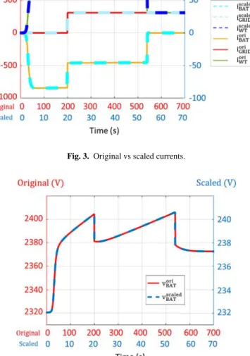
Two simulations are carried out: a first performed at real time without scaling, and a second with current, voltage and time-scaling by a factor of 1/10. All simulation results presented inFigs. 3to6involve two different time scales, a first for “real time scale” (700 s of time horizon) and a second for “accelerated virtual time” (70 s of time horizon). Observing all currents of both studied systems allows not only to validate the current and time-scaling, but also the different steps of the energy management during our textbook case. The dynamics between both models are respected,
Fig. 3. Original vs scaled currents.
Fig. 4. Comparison between original battery voltage and scaled battery voltage.
showing that the two models are in similitude. InFig. 4, the original and scaled battery voltages are presented during the simulation scenario. The similitude on the voltage waveforms is also showed.
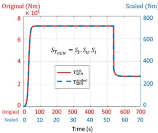
As can be seen inFig. 5, the torque scale factor is a combination of the three scales which means that the generator torque is 1000 times lower in the case of the model. Finally, the evolution of the State of Charge (SoC) inFig. 6is very interesting since this dimensionless variable does not take part in the calculation of the scaled model parameters but is an important indicator especially in terms of dynamics. Then, the energetic behaviour of the battery model between the two simulations is the same. Therefore, the same simulation test has been performed twice, but the second at power levels 100 times smaller and 10 times faster for the time scale.
5. Experimental results 5.1. Experimental set-up
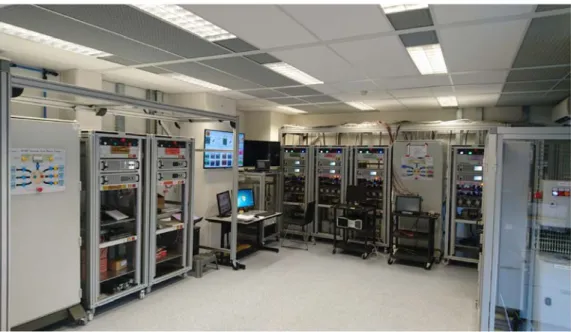
The experimental set-up based on LAPLACE Lab facilities is composed of a common DC bus set at 300 V with a 10.5 kW DC load (this load is also used as a “DC grid emulator”). The wind turbine is emulated using a 15 kW DC power supply while the battery is emulated with a bidirectional DC power supply. These two physical emulators are
Fig. 5. Comparison between original generator torque and scaled generator torque.
Fig. 6. Comparison between original SoC and scaled SoC.
connected to the DC bus through two DC/DC boost choppers. Finally, a resistive load is connected to the DC bus in order to improve the stability of the test bench (Fig. 7).
The emulators’ models are implemented in Matlab-Simulink and the energy management strategy has been implemented on the dSPACE supervisor. The dSPACE manages the overall experimental test bench. A SEFRAM data acquisition system is used to monitor the test bench and record the measurements.
5.2. Test characteristics
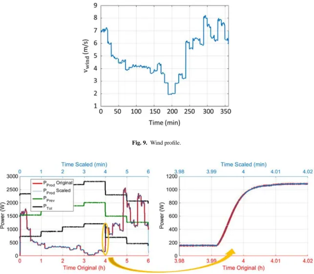
The power of the “scale 1” wind turbine used as our case study is rated at 2MW (Table 4). This power is clearly too high for the test bench. Hence, the nominal power of the wind turbine emulator had to be reduced according to current (1/50) and voltage (1/5) scale factors (Fig. 8).
The total time interval of the wind profile used for the experiment lasts six hours (Fig. 9). The energy management strategy, implemented in the supervisor, is different from that used in simulation. It is based on a heuristic management strategy based on the position of the actual power production with respect to a tolerance layer and to a commitment power, this latter being itself directly linked with the forecast power for the day ahead (day ahead market context) [13].
Fig. 7. LAPLACE Lab facilities: smart microgrids investigation testbench.
Fig. 9. Wind profile.
Fig. 10. Comparison between powers produced by the original wind turbine (St =1) and scaled wind turbine (St=1/60).
5.3. Experimental results
Two tests were carried out: the first one is achieved without time-scaling (St =1) and thus has a real time of six
hours, and the second with a time scale factor equal to 1/60. Consequently, one minute of test in virtual compacted time corresponds to one hour of real time.
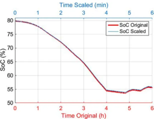
An analysis of the power produced by the wind turbine emulator as well as the evolution of the battery SoC was conducted for both tests. On the one hand, we observe a conservation of dynamics between the produced powers (Fig. 10), and on the state of charge evolution on the other hand (Fig. 11).
On the one hand, the dynamics of the wind turbine power waveforms are the same for both time scales (St=1 and
St=60) and, on the other hand, the SoC evolution of the battery emulator is in similitude (seeFig. 11). Thereby, the
scaling method presented in this paper and adapted to electrical engineering systems, allows conserving the emulator dynamics. However, some technical limits may appear if the time-scaling is so high. For instance, the response time of the emulator depends on the dynamic characteristics of the power supplies. Moreover, the DC/DC converters which allow connecting the emulators on the DC grid could also, according to their control bandwidth, limit the time-scaling. These limits were not studied in this paper.
Fig. 11. Comparison between original SoC (St=1) and scaled SoC (St=1/60).
6. Conclusions
The scaling method presented in this paper represents a first step towards the design of emulators. Based on our state of the art review, the time accelerated concept is a new proposition in the context of HIL experiments.
A methodology to adopt the parameters calculation of a reduced model has been developed involving: – Determination of relevant physical variables;
– Dimensional analysis of the system;
– Choice of the repeating parameters (parameters to be freely scaled); – Determination ofπ-groups;
– Determination of scale factors;
– Calculation of scaled model parameters.
The experimental test has shown that connections between several scaled models are possible, which is an important step in the design of a microgrid.
In addition, an experimental validation of time-scaling has been carried out. The experimental validation underlines the possibility of accelerating tests by keeping similitude factors if the models parameters used are well calculated (according to the similitude theory principle).
Future work will focus on the implementation of real systems (copy-image emulators), and on the compatibility of this concept with time-accelerated test-benches. This will lead us to question on the limits of scaling, especially in the case of time.
References
[1] V. Akhmatov, A. Hede Nielseu, J. Kass Pedersen, Ole Nymann, Variable-speed wind turbines with multi-pole synchronous permanent magnet generators, in: Partie1: Modelling in Dynamic Simulation Tools, Wind Engineering, vol. 27, 2003.
[2] A. Allegre, Reduced-scale-power hardware-in-the-loop simulation of an innovative subway, IEEE Trans. Ind. Electron. 57 (4) (2010) 4765–4770.
[3] M. Belouda, J. Belhadj, B. Sareni, X. Roboam, Battery sizing for a stand alone passive wind system using statistical techniques, in: Proceedings of 8th international multi-conference on systems, signals and devices, Sousse, Tunisia, 2011.
[4] A. Bouscayrol, Different types of hardware-in-the-loop simulation for electric drives, in: Proc. IEEE ISIE, Cambridge, U.K., June 2008, pp. 2146–2151.
[5] A. Bouscayrol, X. Guillaud, P. Delarue, Hardware-in-the-loop simulation of a wind energy conversion system using Energetic Macroscopic Representation, in: IEEE-IECON’05, Raleigh (USA), October 2005.
[6] S. Brennan, On Size and Control: The Use of Dimensional Analysis in Controller Design (Ph.D. thesis), Univ. Illinois at Urbana Champaign, Urbana Champaign, 2002.
[7] P.W. Bridgman, Dimensional Analysis, second ed., Yale University Press, 1931.
[9] J.M. Cabello, E. Bru, X. Roboam, F. Lacressonniere, S. Junco, Battery dynamic model improvement with parameters estimation and experimental validation, in: IMAACA 2015, Bergeggi, Italy, 2015.
[10] C.P. Coutinho, A.J. Baptista, J.D. Rodigues, Reduced scale models based on similitude theory: A review up to 2015, Eng. Struct. 119 (2016) 81–94.
[11] E. Esteban, O. Salgado, A. Iturrospe, I. Isasa, Design methodology of a reduced-scale test bench for fault detection and diagnosis, Mechatronics 47 (2017) 14–23.
[12] Y. Fefermann, S.A. Randi, S. Astier, X. Roboam, Synthesis models of PM Brushless Motors for the design of complex and heterogeneous system, in: EPE’01, Graz, Austria, September 2001.
[13] David Hernandez-Torres, Christophe Turpin, Xavier Roboam, Bruno Sareni, Optimal techno-economical storage sizing for wind power producers in day-ahead markets for island networks, in: Electrimacs 2017, Toulouse, France, July 2017.
[14] S.J. Kwon, Y.G. Son, S.D. Jang, J.H. Suh, J.S. Oh, Ch.H. Chun, C.W. Chung, K.S. Han, D.H. Kim, O.J. Kwon, A simulator for the development of power conversion system for 2MW wind turbine, in: European Wind Energy Conference and Exhibition, Athens, Greece, 2006. [15] T. Letrouve, A. Bouscayrol, W. Lhomme, N. Dollinger, F.M. Calvairac, Reduced scale hardware-in-the-loop simulation of a Peugeot 318
Hybrid4 vehicle, in: 2012 IEEE vehicle power and propulsion conference, VPPC, 9–12 Oct. 2012, pp. 920–925.
[16] J. Martin Cabello, X. Roboam, S. Junco, E. Bru, F. Lacressonniere, Scaling electrochemical battery models for time-accelerated experiments on size-scaled test-benches, IEEE Trans. Power Syst. 32 (6) (2017) 4233–4240.
[17] K.Y. Oh, J.K. Lee, H.J. Bang, J.Y. Park, J.S. Lee, B.I. Epureanu, Development of a 20 kW wind turbine simulator with similarities to a 3 MW wind turbine, Renew. Energy 62 (2014) 379–389.
[18] J. Park, J. Lee, K. Oh, J. Lee, B. Kim, Design of simulator for 3MW wind turbine and its condition monitoring system, in: Proc. IMECS, Hong Kong, Mar. 2010, pp. 930–933.
[19] M.D. Petersheim, S.N. Brennan, Scaling of hybrid-electric vehicle powertrain components for hardware-in-the-loop simulation, Mechatronics 19 (7) (2009) 1078–1090.
[20] T. Szirtes, Applied Dimensional Analysis and Modeling, second ed., Butterworth-Heinemann, 2006.