Bistability between a stationary and an oscillatory dynamo in a turbulent flow of liquid sodium

HAL Id: hal-00492247

https://hal.archives-ouvertes.fr/hal-00492247

HAL is a multi-disciplinary open access archive for the deposit and dissemination of sci-entific research documents, whether they are pub-lished or not. The documents may come from teaching and research institutions in France or abroad, or from public or private research centers.

L’archive ouverte pluridisciplinaire HAL, est destinée au dépôt et à la diffusion de documents scientifiques de niveau recherche, publiés ou non, émanant des établissements d’enseignement et de recherche français ou étrangers, des laboratoires publics ou privés.

Bistability between a stationary and an oscillatory

dynamo in a turbulent flow of liquid sodium

Mickaël Bourgoin, Michaël Berhanu, Basile Gallet, Romain Monchaux,

Philippe Odier, Jean-François Pinton, Nicolas Plihon, Romain Volk, Stéphan

Fauve, Nicolas Mordant, et al.

To cite this version:

Mickaël Bourgoin, Michaël Berhanu, Basile Gallet, Romain Monchaux, Philippe Odier, et al.. Bistability between a stationary and an oscillatory dynamo in a turbulent flow of liquid sodium. Journal of Fluid Mechanics, Cambridge University Press (CUP), 2009, 641, pp.217-226. �10.1017/S0022112009991996�. �hal-00492247�

J. Fluid Mech. (2009), vol. 641, pp. 217–226. _{! Cambridge University Press 2009}c

doi:10.1017/S0022112009991996

217

Bistability between a stationary and an

oscillatory dynamo in a turbulent flow

of liquid sodium

1_{Laboratoire de Physique Statistique, ´Ecole Normale Sup´erieure CNRS UMR8550,}

24 rue Lhomond, F-75005 Paris, France

2_{Service de Physique de l’ ´Etat Condens´e, Direction des Sciences de la Mati`ere CNRS URA 2464,}

CEA-Saclay, F-91191 Gif-sur-Yvette, France

3_{Laboratoire de Physique, ´Ecole Normale Sup´erieure de Lyon, CNRS UMR5672,}

46 all´ee d’Italie, F-69364 Lyon, France

(Received2 June 2009; revised 4 September 2009; accepted 4 September 2009; first published online

16 November 2009)

We report the first experimental observation of a bistable dynamo regime. A turbulent flow of liquid sodium is generated between two disks in the von K ´arm ´an geometry (VKS experiment). When one disk is kept at rest, bistability is observed between a stationary and an oscillatory magnetic field. The stationary and oscillatory branches occur in the vicinity of a codimension-two bifurcation that results from the coupling between two modes of magnetic field. We present an experimental study of the two regimes and study in detail the region of bistability that we understand in terms of dynamical system theory. Despite the very turbulent nature of the flow, the bifurcations of the magnetic field are correctly described by a low-dimensional model. In addition, the different regimes are robust; i.e. turbulent fluctuations do not drive any transition between the oscillatory and stationary states in the region of bistability.

1. Introduction

The magnetic field of most astrophysical objects, like planets, stars and galaxies, is generated by the dynamo effect, which is an instability that converts the kinetic energy of an electrically conducting fluid into magnetic energy. Studies on the geodynamo reveal that global rotation decreases the efficiency of convection (Chandrasekhar 1961) and therefore limits the capability of dynamo action in rapidly rotating flows. However Roberts (1978) suggested that a sufficiently strong magnetic field could create a Lorentz force in balance with the Coriolis force, which may counter the effect of strong rotation. This mechanism predicts a subcritical bifurcation either between a state of no dynamo and a state of strong field or between a weak and a strong

† Present address: ENSTA-UME, chemin de la Huni`ere, 91761 Palaiseau Cedex, France ‡ Present address: LEGI, CNRS UMR 5519, BP53, F-38041 Grenoble, France

¶ Email address for correspondence: Stephan.Fauve@lps.ens.fr " Present address: LEMFI, ENSAM, 151 bld de l’Hˆopital, 75013 Paris, France

F₁

(slow)

F2

(fast)

Sodium at rest

Figure 1. Sketch of the experiment. Two soft iron-bladed disks drive a sodium flow in a cylinder of radius 206 mm and length 524 mm.

field regime. Subcritical transitions have been identified in magnetohydrodynamic numerical simulations of thermal convection in a rotating sphere (Christensen, Olson & Glatzmaier 1999; Morin 2005; Morin & Dormy, submitted) and of body forced flows in a sphere (Fuchs, R¨adler & Rheinhardt 2001) as well as within a periodic box (Ponty et al. 2007) and in Keplerian shear flows (Rincon, Ogilvie & Proctor 2007). In experimental and astrophysical turbulent flows with larger Reynolds numbers (Re! 106_{) and realistic boundary conditions, the existence of subcritical}

dynamo transitions remains an open question. The velocity fluctuations may smooth the transition or suppress bistability. They may also lead the system to explore different regimes successively in time.

Experimental observation of the dynamo instability in fluids has been achieved only recently in Karlsruhe (Stieglitz & M¨uller 2001), Riga (Gailitis et al. 2001) and in a von K ´arm ´an swirling flow of liquid sodium (VKS experiment; Monchaux et al. 2007). A stationary magnetic field has been generated in the Karlsruhe experiment, whereas an oscillatory dynamo has been observed in Riga. In the VKS experiment, various regimes including random reversals (Berhanu et al. 2007; Monchaux et al. 2009) have been observed. All these experiments have displayed continuous primary bifurcations of the magnetic field when the flow velocity is increased. Subcriticality and bistability have not been observed so far. Here we study a turbulent flow of liquid sodium generated between two disks. By varying independently the velocity of each disk, we identify a bistable regime for the magnetic field generated by dynamo action.

The experimental set-up, sketched in figure 1, has been described in Monchaux et al. (2007). A von K ´arm ´an swirling flow is generated by two counter-rotating impellers made of soft iron disks fitted with eight blades (radius R = 154.5 mm, distance between inner faces 371 mm) in an inner copper cylinder (radius Rc= 206 mm, length 524 mm).

We denote the rotation frequencies of the two impellers by F1and F2. The fluid is liquid

sodium (density ρ_{# 930 kg m}−3_{, electrical conductivity σ# 10}7_ohm−1_m−1_{, kinematic}

viscosity ν_{# 10}−6_m2_s−1_{). The flow is surrounded by sodium at rest between the inner}

cylinder and an outer cylinder (radius 289 mm, length 604 mm). The driving motor power is 300 kW, and cooling by an oil circulation inside the wall of the outer copper vessel allows experimental operation at constant temperature in the range 110–160◦_C.

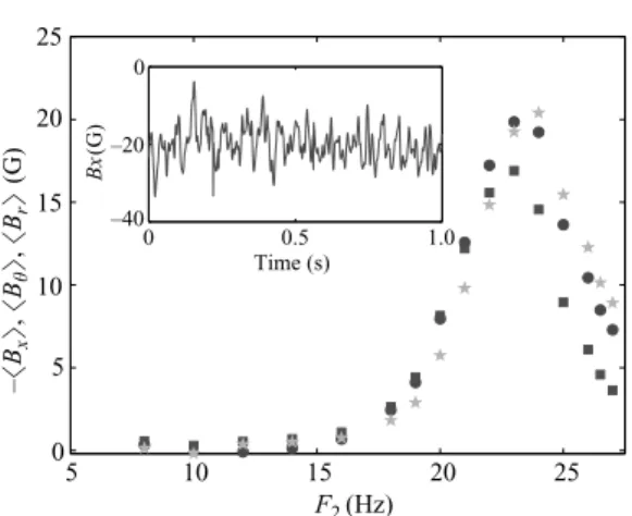
Bistability in a turbulent dynamo 219 10 5 15 20 25 5 0 10 15 20 25 F2 (Hz) –! Bx " , ! Bθ " , ! Br " (G) 0 0.5 1.0 0 –20 –40 Time (s) Bx (G)

Figure 2. Bifurcation diagram of the stationary dynamo generated by varying F2with F1= 0.

The symbols are as follows:!,_−&Bx';",&Bθ'; %, &Br'. The inset shows the corresponding time

series of the component Bx of the stationary dynamo generated for F1= 0 and F2= 24 Hz.

to 5_{× 10}6_{. Correspondingly, magnetic Reynolds numbers R}

mi= 2πµ0σ R2Fi up to 49

at 120◦_{C are reached (µ0 is the magnetic permeability of vacuum). Note that the}

definitions of Re and Rm are different from those given in Monchaux et al. (2007)

and Berhanu et al. (2007), respectively. The values of Re and Rm given here must be

multiplied by K (Rc/R)2, where K = 1.1 is the efficiency of the impellers when one disk

is kept at rest, to recover the value of the latter given in Berhanu et al. (2007). The only modification compared with the set-up described in Monchaux et al. (2007) is the removal of the inner copper ring in the mid-plane. Using cylindrical coordinates, we define x as the coordinate along the axis of the cylinder directed from disk 1 towards disk 2. The radial coordinate is r and θ is the azimuth. The coordinates of the cylinder centre are (x = 0, r = 0). Here we consider experiments in which disk 2 rotates much faster than disk 1. The faster disk drives global rotation in most of the fluid together with radial ejection and axial pumping, generating a one-cell flow with a turbulent shear layer close to the slow disk as illustrated in Ravelet et al. (2004). The magnetic field B is measured with the Hall probes of a three-axis gaussmeter inserted inside the fluid close to the slower disk at the position (x =_{−109 mm, r = 43 mm).} The experiment is operated at a sodium temperature close to 120◦_C.

When the velocity of disk 2 is increased, while disk 1 is at rest, that is to say F1= 0, a magnetic field is generated for F2 larger than 16 Hz, i.e. Rm2 larger than

30. This magnetic field moderately fluctuates around a mean value as shown in the time series plotted in the inset of figure 2. This dynamo is less fluctuating than the stationary dynamo obtained when the two disks exactly counter-rotate. Indeed, for F1= 0 and F2= 24 Hz the standard deviation of the magnetic field normalized as

Brms/&B2'1/2 is around 20 %, whereas it is around 50 % in the counter-rotating case

for F1= F2= 24 Hz. This is related to the smaller turbulent velocity fluctuations when

only one disk is rotated. It has been shown indeed that the ratio of the instantaneous kinetic energy to that of the time-averaged flow is about twice as large in the counter-rotating case than in the one-disk configuration (Cortet et al. 2009). Increasing the velocity of the disk by steps of 0.5 Hz, a stationary dynamo is maintained. The time average of each component of the magnetic field _&Bi' is displayed as a function of

F2 in figure 2. The three components of the magnetic field are of the same order

22 24 26 28 0 2 4 F1 (Hz) F₂ (Hz) F₂ (Hz) Path 1 Path 2 25.0 25.5 26.0 26.5 0 1 2 Path 3

Figure 3. Paths followed in the parameter space (F2, F1):!, stationary dynamos; %, oscillatory

dynamos. Note that for (26, 0), depending on the path, either an oscillatory or a stationary dynamo can be obtained.

0 50 –50 –100 100 (a) (b) Bi (G) 260 280 300 320 340 0 1 2 3 F1 (Hz) Time (s)

Figure 4. Time series for the oscillatory dynamo. (a) Magnetic field components as a function

of time. The colours are as follows: blue, Bx; red, Bθ; green, Br. (b) Velocity of the slow disk

F1as a function of time. At t = 295 s, the velocity of disk 1 is set to F1= 0 while F2= 26 Hz.

and azimuthal components. The sign of _&Bx'&Bθ' is set by the one of differential

rotation, as when the disks are in exact counter-rotation. Both solutions B and _−B can be observed. There is an intensity difference (of the order of 5 G) between these branches, an effect possibly due to induction from the ambient magnetic field. The time-averaged amplitude of the magnetic field_&B2_'1/2_{grows up to 35 G for F}

2# 24 Hz

and then decreases for larger velocities.

When disk 1 slowly counter-rotates compared with disk 2, a periodic dynamo is generated. To investigate the relative stability of the stationary and oscillatory regimes, we follow three different paths (sketched in figure 3) in parameter space, each ending on the line (F2, 0) where only disk 2 rotates. Path 1 has been presented above. The

two others are performed by slowing down disk 1, disk 2 being kept at a fast rotation rate (resp. at 26 and 26.5 Hz). We now describe the evolution of the dynamo when following path 2. If F2= 26 Hz and F1 is larger than 1 Hz, a periodic dynamo takes

place, the time series of which is displayed in figure 4. At time t = 295 s, disk 1 is stopped, and the magnetic field tends towards a stationary value after transient damped oscillations. This stationary magnetic field is similar to the field produced when following path 1. The damped oscillations indicate that the corresponding fixed point is linearly stable with complex eigenvalues.

Bistability in a turbulent dynamo 221 0 50 –50 –100 100 (a) (b) Bi (G) 440 460 480 500 520 540 560 0 0.5 –0.5 1.0 1.5 Time (s) F1 (Hz)

Figure 5. Time series for the oscillatory dynamo. (a) Magnetic field components as a function

of time. The colours are as follows: blue, Bx; red, Bθ; green, Br. (b) Velocity of the slow disk

F1as a function of time. At t = 480 s, the velocity of disk 1 is set to F1= 0 while F2= 26.5 Hz.

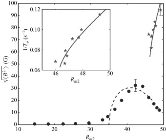
10 20 30 40 50 0 10 20 30 40 50 60 70 80 90 100 46 48 50 0.06 0.08 0.10 0.12 Rm2 Rm2 1/ To (s –1) ! B 2 " (G) √

Figure 6. Amplitude of the magnetic field &B2_'1/2 _{as a function of R}

m2 for Rm1= 0. The

inset shows the frequency of the oscillatory dynamo. The symbols are experimental values:

!, stationary dynamo; %, oscillatory dynamo. The length of the error bars is obtained from

the dispersion of the measurements performed for the same parameter values. The lines are obtained from the solutions of the dynamical system defined by (1): ——, oscillatory solution; − − −, stationary solution.

To follow path 3, we start with F2= 26.5 Hz and F1! 1 Hz. The dynamo is then

periodic. When stopping disk 1, it is possible to maintain a periodic dynamo as can be seen in figure 5. We then decrease F2, and the system remains in periodic

dynamo regime for F2 down to 25.75 Hz. A stationary dynamo is finally recovered for

F2= 25.25 Hz. The period of the oscillatory dynamo roughly increases from 9 to 15 s

when F2 is varied from 27 to 25.5 Hz. The frequency does not vanish for the smallest

velocity at which the oscillations can be maintained, as can be seen in the inset of figure 6. The three components of the magnetic field are non-zero and are of similar amplitude. During most of the period, the axial field is of opposite sign with respect

to the azimuthal and radial fields, as is the case in the stationary regime. There is a small phase shift between the three components, the radial one being delayed by less than one tenth of a period. Measurements at other positions (not described here) have shown that the magnetic field oscillates with roughly the same phase within the experiment. As expected for a bistable regime, this oscillatory dynamo has also been observed when one disk is at rest if the velocity of the other disk is increased by larger steps (3 Hz). However the oscillatory branch is more easily observed when the flow is first driven with both disks rotating.

From the former paths in the parameter space, we can state that two different dynamo regimes are observed for the same values of the control parameters. This proves the existence of two locally stable dynamo branches. We measure that the domain of bistability extends from 25.5 to 27 Hz in F2. Driving one disk at 27 Hz, the

other one being at rest, requires all the available power for one disk, roughly 150 kW. This power limitation does not allow us to reach higher frequencies, but we expect the interval of bistability to be wider. A bifurcation curve based on the norm of the magnetic field is plotted in figure 6. The amplitudes of the two branches strongly differ. The oscillatory dynamo generates a field with energy density roughly 10 times larger than that of the stationary dynamo. However, within measurement accuracy, there is no noticeable effect on the power delivered by the motor (with the change being less than 3 %).

We note that for the stationary regime and during most of the period of the oscillatory one, the axial and azimuthal components of the magnetic field are of opposite signs. This is in agreement with a mechanism of magnetic field generation put forward in P´etr´elis, Mordant & Fauve (2007): the flow of the fluid radially expelled by the disk is strongly helical and generates an α effect localized close to the disk. This α effect converts the azimuthal field into the axial field. Differential rotation is responsible for the ω effect that converts the axial magnetic field into the azimuthal one. This mechanism has been studied by Laguerre et al. (2008) in the framework of mean-field magnetohydrodynamics. It has been found that the magnitude of α needed to obtain the dynamo is much too large. This has been confirmed by Giesecke et al. (forthcoming). The possible role of the iron impellers has been also taken into account, and it has been shown that a smaller value of α is needed for dynamo action (Giesecke, Stefani & Gerbeth, forthcoming). However, kinematic calculations performed without using any α parameterization have shown that taking into account non-axisymmetric vortices along the blades fairly well describes the experimental results (Gissinger, forthcoming). More measurements are necessary to fully describe the structure of the field and the amplification mechanisms. Nevertheless, our explanation for the bistability (detailed in the following) confirms the fact that the same effects are at work for both the stationary and the oscillatory regime.

To identify the dynamics that leads to bistability between the two regimes we perform a phase-space study of the magnetic field. To wit we plot the radial magnetic field as a function of the azimuthal one. In figure 7(a), we display the evolution corresponding to different initial conditions and F1= 0, F2= 26 Hz. In one case the

solution spirals towards a fixed point; in the other case it describes a limit cycle. We note that the fixed point, its opposite and the B = 0 unstable solution are located inside the limit cycle. Figure 7(b) represents the evolution of the limit cycle when F2

is varied. It is clear that when F2 is decreased the limit cycle comes closer to B = 0.

These results can be understood as resulting from the competition between two modes of magnetic field in the vicinity of a codimension-two bifurcationor, more precisely, of a bifurcation for a linear problem with a double zero eigenvalue.

Bistability in a turbulent dynamo 223 0 50 –50 0 50 (a) (b) –50 –50 Bθ (G) 0 50 –50 Bθ (G) Br (G) 0 50

Figure 7. Plot of a cut in phase space [Bθ(t), Br(t)] for different measurements with F1= 0 Hz.

(a) F2= 26 Hz. The blue (resp. red) line is made from the time series of figure 4 (resp. figure 5)

and corresponds to initial conditions attracted towards a fixed point (resp. a limit cycle). (b)

F2= 27 Hz (blue) and F2= 25.5 Hz (black). Note the initial evolution that circles around the

fixed point in the upper right part of the plot before describing the limit cycle.

Following P´etr´elis & Fauve (2008), we assume that the dynamics of the magnetic field results from the competition between two magnetic modes and write the magnetic field as B = A1(t) B1(r) + A2(t) B2(r) where Bi are the spatial structures of the modes

and Ai their amplitudes. Dynamics of the magnetic field is then reduced to that of

A= A1+ iA2. The amplitude equation for A should be invariant when A→ −A, since

the equations of magnetohydrodynamics are invariant when B_{→ −B. When the two} modes are near criticality, we obtain up to the leading-order nonlinearities

˙

A= (δ1+ iδ2)A + (ν1+ iν2) ¯A+ β1A3+ β2A2A¯+ β3A ¯A2+ β4A¯3. (1)

Equations similar to (1) occur in many different contexts. In particular, they describe strong resonances in space (Coullet 1986) or in time (Chiffaudel & Fauve 1987) for pattern-forming instabilities. Their bifurcation diagram has been widely studied (Arnold 1982; Gambaudo 1985).

In the general case, the coefficients βi are complex and δ1, δ2, ν1 and ν2 are real.

They depend on the experimental parameters. It has been shown that when δ1is large

enough such that the amplitude of A can be adiabatically eliminated, transitions from stationary to periodically reversing dynamos result from a saddle-node bifurcation. In addition, if turbulent fluctuations are modelled by multiplicative noise, (1) describes random reversals and bursts observed in the VKS experiment (P´etr´elis & Fauve 2008, P´etr´elis et al. 2009).

When δ1= 0 and δ22= ν12+ ν22, (1) has a codimension-two bifurcation point with a

double-zero eigenvalue and only one eigenvector; i.e. the system is close to both a stationary and a Hopf bifurcation. Indeed, the eigenvalues of the linear part of the equation are δ1±

! ν₁2+ ν2

2 − δ22. Up to a rotation and a change of time scale, the

linear part of (1) can be reduced to ˙X= Y and ˙Y= 0, where X + iY = Ae−i(φ/2+π/4) with δ2eiφ= ν1+ iν2. The phenomenology of this codimension-two bifurcation is well

documented (Guckenheimer & Holmes 1983). At the bifurcation, the normal form can be written as ˙X= Y and ˙Y=_±X2_{Y− X}3_{, up to a close-to-identity transformation}

and rescaling of time and amplitudes. When the two nonlinear terms of the normal form saturate the instability, the oscillation appears via a saddle-node bifurcation that creates a pair of limit cycles, a stable and an unstable one. These limit cycles encircle the three stationary solutions (B = 0 and the two bifurcated solutions_±Bs). Once the

limit cycles are created and as long as the stationary bifurcated solutions are stable, the system displays bistability between the stationary and the oscillatory solutions.

To illustrate this scenario, we compare the experimental results with the solution of (1) when a simple variation of the coefficients as a function of Rm2 is prescribed.

For simplicity, we keep only the nonlinear term that does not break phase invariance; i.e. we take β1= β3= β4= 0. In order to reduce further the number of fitting

parameters, we note that the phase-space representation of the system is elongated along the diagonal Br= Bθ (see figure 7). Similarly, the three components of the

magnetic field remain comparable. This implies that one of the two modes, say B1, is larger than the second mode at the location at which the measurements

are performed. Therefore the amplitude A1 can be considered as providing a good

estimation of the magnetic field at the measurement point. The remaining coefficients are then chosen such that the stationary and oscillatory instability thresholds, the oscillation amplitudes and frequencies and the maximum of the stationary solution amplitude, are correctly described. This is achieved by setting ν1= 0.27, ν2= 0.52,

δ1= 0.043Rm2− 1.74, δ2= 1.45− 0.026Rm2 and β2= 10−5(−0.95 + 1.9 i). We obtain

from (1) that the stationary solution bifurcates for Rm2= 35.7 and displays bistability

with the oscillatory solution when Rm2! 46.1. We display "

&B2

' and the period of the oscillatory solutions in figure 6. The imperfection of the bifurcation observed in the experimental data may be attributed to the remanent magnetization of the disks. Taking into account this imperfection as well as the experimental error bars, we observe that the model describes the measurements fairly well. In other words, not only the phenomenology of the successive bifurcations but also some quantitative aspects are captured by this low-dimensional approach. This shows that the dynamical regimes observed in a fully turbulent flow result from the competition between two modes of magnetic field. Indeed, even though the Reynolds number is larger than 106_,

the magnetic Reynolds number remains close to onset, and the dynamics is governed by the small number of magnetic modes contained in the central manifold.

We emphasize that the scenario described here is different from the one observed for values of Fi closer to exact counter-rotation. In that case, the magnetic field evolves

from a stationary to a periodic behaviour when one of the velocities is changed (Ravelet et al. 2008). There is no bistability, and the fixed point associated with the stationary behaviour belongs to the periodic orbit. In the vicinity of this bifurcation, turbulent fluctuations drive random reversals by excitability. In the present case, both the stationary and time periodic regimes coexist for the same parameter values. When the turbulent flow of liquid sodium is driven by the fast rotation of one disk, the magnetic field remains in one of the states, and the turbulent fluctuations are not sufficient to trigger random transitions between the two regimes on an observation time larger than hundreds of ohmic diffusive times or thousands of hydrodynamic eddy turnover times. The coexistence of a stationary and an oscillatory regime has been also observed when both disks rotate at different frequencies (for instance F1= 16.75 Hz, F2= 25.25 Hz). However, in that case random transitions between the

stationary and the oscillatory regime are observed without changing the control parameters (see figure 3.69 in Berhanu 2008). This can be due either to the larger intensity of turbulent fluctuations when the two impellers are counter-rotating at comparable frequencies or to the proximity of the fixed point and the limit cycle in phase space. In any case, we stress that the low-dimensional dynamics of the magnetic field is very robust. These features can be understood as resulting from the coupling between two modes of magnetic field close to their onset of instability. Far from

Bistability in a turbulent dynamo 225 the codimension-two point of the amplitude equation (1), we have a transition from a stationary state to a time-periodic one through a saddle-node bifurcation. In the vicinity of the codimension-two point, the bistable behaviour is observed.

Finally, we emphasize that the dynamo regimes observed in the VKS experiment strongly differ from the ones computed using the mean flow alone. It is necessary to take into account non-axisymmetric fluctuations of the flow, and these fluctuations are turbulent. The validity of the low-dimensional description of the dynamics of the magnetic field relies the small number of magnetic modes competing in the vicinity of the dynamo threshold.

We are indebted to M. Moulin, C. Gasquet, J.-B. Luciani, A. Skiara, D. Courtiade, J.-F. Point, P. Metz and V. Padilla for their technical assistance at various stages of the experiment. This work is supported by the following French institutions: Direction des Sciences de la Mati`ere and Direction de l’Energie Nucl´eaire of CEA, Minist`ere de la Recherche, and Centre National de Recherche Scientifique (ANR 08-0039-03). The experiment was operated at CEA/Cadarache DEN/DTN.

REFERENCES

Arnold, V. 1982 Geometrical Methods in the Theory of Ordinary Differential Equations. Springer. Berhanu, M. 2008. Magn´etohydrodynamique turbulente dans les m´etaux liquides. PhD thesis,

Universit´e Pierre et Marie Curie, Paris, p. 105.

Berhanu, M., Monchaux, R., Fauve, S., Mordant, N., P´etr´elis, F., Chiffaudel, A., Daviaud, F., Dubrulle, B., Mari´e, L., Ravelet, F., Bourgoin, M., Odier, Ph., Pinton, J.-F. & Volk, R. 2007 Magnetic field reversals in an experimental turbulent dynamo. Europhys. Lett. 77, 59001.

Chandrasekhar, S. 1961 Hydrodynamic and Hydromagnetic Stability. Clarendon.

Chiffaudel, A. & Fauve, S. 1987 Strong resonance in forced oscillatory convection. Phys. Rev. A 35, 4004–4007.

Christensen, U. R., Olson, P. & Glatzmaier, G. A. 1999 Numerical modelling of the geodynamo: a systematic parameter study. Geophys. J. Intl 138, 393–409.

Cortet, P.-P., Diribarne, P., Monchaux, R., Chiffaudel, A., Daviaud, F. & Dubrulle, B. 2009 Normalized kinetic energy as a hydrodynamical global quantity for inhomogeneous anisotropic turbulence. Phys. Fluids 21, 025104.

Coullet, P. 1986 Commensurate-incommensurate transition in nonequilibrium systems. Phys. Rev. Lett. 56, 724–727.

Fuchs H., R¨adler K.-H. & Rheinhardt, M. 2001 Suicidal and parthenogenetic dynamos. In

Dynamo and Dynamics, a Mathematical Challenge (ed. P. Chossat, D. Armbuster & I. Oprea), pp. 339–347. Kluwer Academic.

Gailitis, A., Lielausis, O., Platacis, E., Dement’ev, S., Cifersons, A., Gerbeth, G., Gundrum, T., Stefani, F., Christen M. & Will, G. 2001 Magnetic field saturation in the Riga dynamo experiment. Phys. Rev. Lett. 86, 3024–3027.

Gambaudo, J. M. 1985 Perturbation of a Hopf bifurcation by an external time-periodic forcing. J. Diff. Eq. 57, 172–199.

Giesecke, A., Nore, C., Plunian, F., Laguerre, R., Ribeiro, A., Stefani, F., Gerbeth, G., L´eorat, J. & Guermond, J.-L. 2009a Generation of axisymmetric modes in cylindrical kinematic mean-field dynamos of VKS type. Geophys. Astrophys. Fluid Dyn. In press.

Giesecke, A., Stefani, F. & Gerbeth, G. 2009b Role of soft-iron impellers on the mode selection in the VKS dynamo experiment. Phys. Rev. Lett. Submitted.

Gissinger, C. 2009 A numerical model of the VKS experiment. Europhys. Lett. 87, 39002. Guckenheimer, J. & Holmes, P. 1986 Nonlinear Oscillations, Dynamical Systems and Bifurcations

of Vector Fields. Springer.

Laguerre, R., Nore, C., Ribeiro, A., L´eorat, J., Guermond, J.-L. & Plunian, F. 2008 Impact of impellers on the axisymmetric magnetic mode in the VKS2 dynamo experiment. Phys. Rev. Lett. 101, 104501, 219902.

Monchaux, R., Berhanu, M., Aumaˆıtre, S., Chiffaudel, A., Daviaud, F., Dubrulle, B., Ravelet, F., Fauve, S., Mordant, N., P´etr´elis, F., Bourgoin, M., Odier, Ph., Pinton, J.-F., Plihon, N. & Volk R. 2009 The von K ´arm ´an sodium experiment: turbulent dynamical dynamos. Phys. Fluids 21, 035108.

Monchaux, R., Berhanu, M., Bourgoin, M., Moulin, M., Odier, Ph., Pinton, J.-F., Volk, R., Fauve, S., Mordant, N., P´etr´elis, F., Chiffaudel, A., Daviaud, F., Dubrulle, B., Gasquet, C. & Mari´e, L. 2007 Generation of a magnetic field by dynamo action in a turbulent flow of liquid sodium. Phys. Rev. Lett. 98, 044502.

Morin, V. 2005 Instabilit´es et bifurcations associ´ees `a la mod´elisation de la G´eodynamo. PhD thesis, Universit´e Pierre et Marie Curie. Paris.

Morin, V. & Dormy, E. 2009 Weak and strong field dynamos. Phys. Rev. Lett. Submitted. P´etr´elis, F. & Fauve, S. 2008. Chaotic dynamics of the magnetic field generated by dynamo action

in a turbulent flow. J. Phys. Condens. Matt. 20, 494203.

P´etr´elis, F., Fauve, S., Dormy, E. & Valet, J.-P. 2009 A simple mechanism for the reversals of Earth’s magnetic field. Phys. Rev. Lett. 102, 144503.

P´etr´elis, F., Mordant, N. & Fauve, S. 2007 On the magnetic fields generated by experimental dynamos. Geophys. Astrophys. Fluid Dyn. 101, 289–323.

Ponty, Y., Laval, J.-P., Dubrulle, B., Daviaud, F. & Pinton, J.-F. 2007 Subcritical dynamo bifurcation in the Taylor–Green flow. Phys. Rev. Lett. 99, 224501.

Ravelet, F., Berhanu, M., Monchaux, R., Bourgoin, M., Odier, Ph., Pinton, J.-F., Plihon, N., Volk, R., Fauve, S., Mordant, N., P´etr´elis, F., Aumaˆıtre, S., Chiffaudel, A., Daviaud, F., Dubrulle, B. & Mari´e, L. 2008 Chaotic dynamos generated by a turbulent flow of liquid sodium. Phys. Rev. Lett. 101, 074502.

Ravelet, F., Mari´e, L., Chiffaudel, A. & Daviaud, F. 2004 Multistability and memory effect in a highly turbulent flow: experimental evidence for a global bifurcation. Phys. Rev. Lett. 93, 164501.

Rincon, F., Ogilvie, G. I. & Proctor, M. R. E. 2007 Self-sustaining nonlinear dynamo process in Keplerian shear flows. Phys. Rev. Lett. 98, 254502.

Roberts, P. H., 1978 Magneto-convection in a rapidly rotating fluid. In Rotating Fluids in Geophysics (ed. P. H. Roberts & A. M. Soward), pp. 421–435. Academic.

Stieglitz, R. & M¨uller, U. 2001 Experimental demonstration of a homogeneous two-scale